
Recently, I needed a certain type of 3D-illustration for a post series about cosmology. I wanted to show a 2-dimensional manifold above a mesh grid with respective coordinate lines on the surface. In front of the surface I wanted to place some opaque spheres. Such illustrations are often used in physics to demonstrate the effect of some objects on a physical quantity – e.g. of spherical bodies on the gravitational potential or on a component of the metric tensor of space-time.
The simple problem to get a correct rendering of objects along a defined line of view upon a 3D scene posed a problem for Matplotlib’s 3D renderer for multiple objects in a 3D axis frame (created by ax = plt.axes(projection=’3d’)). The occlusion of objects was displayed wrongly for most view ports and viewing angles.
In this post, I briefly want to outline how this problem can be solved with the help of S3Dlib. As a beginner regarding the use of S3Dlib, I had to overcome some problems there, too. So, this small exercise with some options of S3Dlib might be interesting for some readers which want to use Python and Matplotlib for rendering simple 3D scenes.
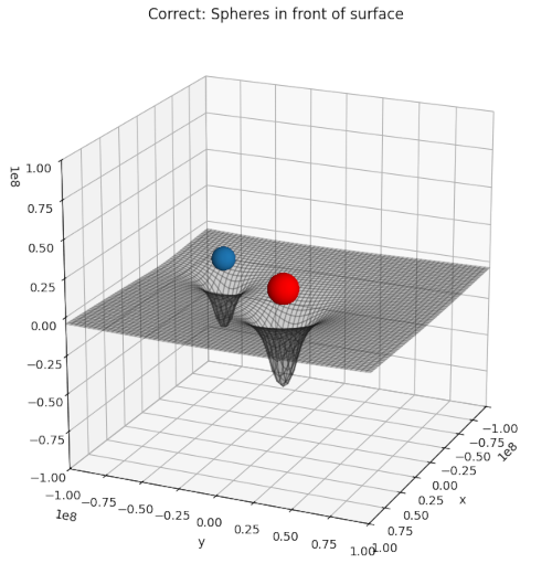
The following plot shows what I wanted to achieve:
Problem with 3D-rendering in Matplotlib
I was a bit astonished to notice that the task of displaying objects in front of a 2-dim surface (in my case a wireframe based on a meshgrid) led to major problems with the Matplotlib’s renderer. One can easily plot both a perfect spherical surface and a 2-dimensional manifold with Matplotlib in separate 3D axis-frames. However, when one places such objects in one and the same 3D ax-frame, it does not seem to be possible to get the 3D-occlusion of the surface/wireframe by opaque spheres somewhat above or in front of the surface/wireframe right.
The meshgrid or a related surface [z = z(x,y)] always occluded a sphere – in my case despite coordinate settings of the sphere such that it was placed in front of the surface along the defined line of view. See the image below:
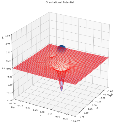
The blue sphere with a radius of 1.0e7 was positioned at (x=0, y=0, z≈3.8e7) – clearly in front and above of the surface, whose edges are below the (z=0)-plane. Nevertheless, Matplotlib rendered the surface as if it were located in front of the sphere.
Other users had similar problems with the order of objects occluding or even intersecting one another. See [1], [2].
In some discussions the use of Mayavi is recommended. However, I got serious trouble with installing it on my laptop system. I left this for future investigation and turned to S3Dlib.
S3Dlib as an extension to Matplotlib
S3Dlib is a kind of supplemental library to Matplotlib. On the one side it makes life a bit easier when you want to generate elementary 3D-objects, on the other side its basically polygonal approach to create surfaces in a 3-dimensinal space allows for a correct rendering together with the function “ax.add_collection3d()”. Most 3D objects in S3Dlib must technically be understood as instances of a child-class “Surface3DCollection” of Matplotlib’s class “Poly3DCollection“. But, instead going into the theory and techniques of using closed flat 2-dim polygons for surface constructions in 3D, let us turn to an example code and see how we can practically use these classes step by step.
Code for experiments with S3Dlib
In S3Dlib you normally create a 3D-sphere in a polar coordinate system. The data for the resulting flat polygons making the surface are incorporated in special objects. However, for reasons of an instructive visualization, surfaces may instead be created in Cartesian coordinates. With S3Dlib we can, fortunately, enforce coordinate transformations in a very simple way. This will help us later to merge objects with polygonal data and render them afterward as one super-object via invoking add_collection3d(). For such super collections the 3D rendering of all the overlapping flat polgyonal figures is done consistently.
Let us look at a simple code example. I split the code in several section. I start with imports and some control parameters:
Imports and parameters
import numpy as np
import matplotlib.pyplot as plt
from mpl_toolkits.mplot3d import axes3d
from matplotlib import cm
import matplotlib.colors as colors
import s3dlib.surface as s3d


# Parameters
# *************
b_test    = True # True: show test sphere , False: Show real "transformed" spheres
b_2sph    = True  # 2 spheres, relevant only for b_test = True

# Constants for Grav. Pot of 2 bodies
# ~~~~~~~~~~~~~~~~~~~~~~~~~~~~~~~~~~~
G = 6.67430e-11 # Gravitational constant
# big body - will be centered
M = 5.972e24; R = 6371e3 * 1.5  # Massof the Earth, Radius of earth stretched
#small body
# MS = 7.348e22; RS = 3.474e3 # moon
MS = 0.5*M; RS = 0.75 * R #  effect moon to small

# Distances to 2nd body - for illustration
DXS = -3.8 * R
DYS =  1.6 * DXS

# big and small sphere
dx_sph_b = 0.0;   dy_sph_b = 0.0;   dz_sph_b = 0.0
dx_sph_s = DXS;   dy_sph_s = DYS;   dz_sph_s = 0.0

# test spheres
dx_sph_t  = -0.00e8;  dy_sph_t  =  0.0e8;  dz_sph_t  = 0.1e8
dx_sph_t2 = +0.40e8;  dy_sph_t2 =  0.8e8;  dz_sph_t2 = 0.25e8

# direction of light ray for 3D illustration
lightdir =(0.75,1,0.6)
We control the position of two bodies – a big one at (x=0, y=0, z=0) and one more compact body with less mass at some distance from the bigger one. We define some “geometry” functions to get a smooth gravitational potential inside and outside the spheres.
Python Functions
Next we want to generate a 2-dim manifold in Cartesian coordinates. For reasons of simplicity, I just used the gravitational potential as it gives us a smooth variation depending on (x,y)-coordinates. (We ignore the variation with the 3rd dimension). See the function g_pot_xy(). Furthermore, another function is required to create a sphere’s surface (via polygons) – either in polar or Cartesian coordinates. S3Dlib offers a a basic function to create a sphere based on polar coordinates. The function “sphere2cart()” below is used to afterward make a transformation of the surface data to Cartesian coordinates.
# Function to create grav. potential based on Cartesian coordinates
#~ ~~~~~~~~~~~~~~~~~~~~~~~~~~~~~~~~~~~~~~~~~~~~~~~~~~~~~~~~~~~~~~~~
def g_pot_xy(xyz, delta=0.05) :
    x,y,z = xyz
    X = x * 1.e8
    Y = y * 1.e8

    # calc distaces
    d  = np.sqrt( X**2 + Y**2 )
    ds = np.sqrt( ( X - DXS )**2 + ( Y - DYS )**2 )

    Z1 = G * M/2./R**3 * (d**2 - 3.*R**2)
    Z2 = - G * M / (d +1.e-3)
    Z = np.where ( d < R, Z1, Z2)

    Z3 = G * MS/2./RS**3 * (ds**2 - 3.*RS**2)
    Z4 = - G * MS / ( ds + 1.e-3)  # Gravitational potential
    ZS = np.where ( ds < RS, Z3, Z4)

    Z += ZS

    return X,Y,Z

# Function to create sphere in Cartesian coordinates
# ~~~~~~~~~~~~~~~~~~~~~~~~~~~~~~~~~~~~~~~~~~~~~~~~~~
def sphere2cart(xyz) :
    x,y,z = xyz
    T = -np.pi*(x+1)
    P = np.pi*(y+1)/2
    R = np.ones(len(z)).astype(float)
    XYZ = s3d.SphericalSurface.coor_convert([R,T,P],True)
    return XYZ
Note that the function “g_pot_xy” superimposes the effects of two bodies [ … by the way: ChatGPT-4 (free version) had programmed this functions wrongly, when asked to provide respective Python code …]. Regarding the 2nd function we are happy that S3Dlib offers a simple function for the transformation to Cartesian coordinates. This allows us an adaption of the resulting arrays of construction data both for the surface and the spheres – not only regarding certain dimensions, but also the mathematical meaning of the coordinates and z-values. More information on the method “coor_covert()” is found here.
Construction of test spheres
# +++++++++++++++++++++++++++++++++++++++++++++++++++++++++++
rez = 5
rez_sph = 5

# 1. Construct polygonal collection data of test spheres in polar coordinates
# ~~~~~~~~~~~~~~~~~~~~~~~~~~~~~~~~~~~~~~~~~~~~~~~~~~~~~~~~~~~~~~~~~~~~~~~~~~~~~
if b_test:
    sph_t  = s3d.SphericalSurface(rez_sph, color='yellow')
    sph_t2 = s3d.SphericalSurface(rez_sph, color='orange')
    # Scale and place test sphere above plane
    sph_t.transform( scale=1.* R,  translate=[dx_sph_t,  dy_sph_t,  dz_sph_t]).shade()
    sph_t2.transform(scale=1.* RS, translate=[dx_sph_t2, dy_sph_t2, dz_sph_t2]).shade()
We define a resolution (rez_sph) for the construction of two test spheres (and rez for the surface). You may choose rez_sph=4 to save some computational time during a test. The transform function executes both a scaling to the given geometrical context (1.e8 as a natural length unit in ur case) and a vector translation to new coordinates. The shading of the surface is done by a method “shade()“. Check the S3Dlib-documentation [3] for parameters of this function.
Construction of the 2-dim surface (= variation gravitational potential with x,y)
# 2. Setup and map polygonal collection data for the surface object in Cartesian coordinates
# ~~~~~~~~~~~~~~~~~~~~~~~~~~~~~~~~~~~~~~~~~~~~~~~~~~~~~~~~~~~~~~~~~~~~~~~~~~~~~~~~~~~~~~~~~
oper = [g_pot_xy] # array for geometries

Sc = colors.to_rgba('red', 0.25)
Fc = colors.to_rgba('#333', 0.22)

surface =  s3d.PlanarSurface(rez, basetype='squ', color=Sc, facecolor=Fc, edgecolor='r', lw=0.6, antialiased=True)
surface.map_geom_from_op( oper[0] )
sur = surface.shade(direction=lightdir, flat=False)
We use the elementary method PlanarSurface of S3Dlib to create the manifold. Note that there are other methods instead of ‘squ’ to construct connected closed 2D-polygons to build the surface. Another more complex approximation of the surface by planar polygons is “quad”. See the S3Dlib documentation for more information. You may try out “quad” – and experience an improved resolution , but also an increase in required CPU time.
The geometrical data of our 2-dim manifold are invoked by providing a reference to g_pot_xy. (The use of an array is overkill here, but it would allow in future versions to quickly shift to other prescriptions of the surface data.) There are, however, other methods to define a surface with S3Dlib than by just calling a function. You can e.g. use z-data given for a meshgrid. Read the S3Dlib guides and API-documentation for more information [3]. Shading of the surface is done with assuming a certain direction of respective light-rays.
Two massive spheres, a big one and a smaller one, in front of the 2D-surface
# 3. Setup and map polygonal collection data of spheres in Cartesian coordinates
# ~~~~~~~~~~~~~~~~~~~~~~~~~~~~~~~~~~~~~~~~~~~~~~~~~~~~~~~~~~~~~~~~~~~~~~~~~~~~~~~
color_sph_b = "red"
fac_b = 1.; fac_s = 0.75
if not b_test:
    sph_b_cart = s3d.PlanarSurface(rez, basetype='squ', color=color_sph_b)
    sph_b_cart.map_geom_from_op( sphere2cart )
    sph_b_cart.transform(scale=fac_b*R)
    sph_b_cart.transform(translate=[dx_sph_b, dy_sph_b, dz_sph_b]).shade(direction=lightdir)

    sph_s_cart = s3d.PlanarSurface(rez, basetype='squ')
    sph_s_cart.map_geom_from_op( sphere2cart )
    sph_s_cart.transform(scale=fac_s*R)
    sph_s_cart.transform(translate=[dx_sph_s, dy_sph_s, dz_sph_s]).shade(direction=lightdir)
In this case we have to do the geometry mapping by our function sphere2cart. The reason is that the resulting objects (and their contained arrays) have to be aligned. See below.
Combination of the collections containing the geometry data of the objects
A very important step to the solution is to stack the various Surface3DCollection-objects, which contain the geometrical information of the surface and our spheres, into a kind of super collection object. This can be done by an overloaded “+” operator (or a respective __add__-function).
# 4. Combine polygonal collection data of our objects in one super-collection
# ~~~~~~~~~~~~~~~~~~~~~~~~~~~~~~~~~~~~~~~~~~~~~~~~~~~~~~~~~~~~~~~~~~~~~~~~~~~~~
# test scene
if b_test:
    surf = sur
    if b_2sph:
        sphc = sph_t + sph_t2
    else:
        sphc = sph_t

# full scene
else:
    surf = sur + sph_b_cart + sph_s_cart
In our case, I called the Python object containing the data (polygons) of both our spheres and surface object for the full scene “surf“. This collection of closed polygons will later be rendered in the 3D axes frame via the function add_collection3d().
Plotting in 3D axes frame
# 5. Plot figure, 3D-ax and render our super-collections
# ~~~~~~~~~~~~~~~~~~~~~~~~~~~~~~~~~~~~~~~~~~~~~~~~~~~~~~

fig = plt.figure(figsize=(10,8))
ax = plt.axes(projection='3d')
s3d.auto_scale(ax,surface)

ax.dist = 10

# viewing angles
elev_1 = 20
#elev_1 = 0
azim_1 = 24
ax.view_init(elev=elev_1, azim=azim_1)

ax.set_box_aspect((4., 4., 4.))

D = 1.e8
ax.set_xlim(-D, D)
ax.set_ylim(-D, D)
ax.set_zlim(-D, D)

# plot collections
ax.add_collection3d(surf)
if b_test:
    ax.add_collection3d(sphc)

ax.set_xlabel('x')
ax.set_ylabel('y')
if b_test:
    ax.set_title('Wrong: Surface covers test sphere (polar coord.)')
else:
    ax.set_title('Correct: Spheres in front of surface')

#fig.tight_layout()
plt.show()
Note that we use the Matplotlib function “ax.add_collection3d()” to do the final rendering of the overlapping 2-dim closed polygons of our objects.
Note further that for b_test=True “surf” only contains the 2-dim surface; so the spheres are independently rendered in this case. For b_test=False “surf” instead contains the geometry information of all objects to be displayed.
S3Dlib: No difference to Matplotlib when spheres and surface are based on different basic objects in different coordinate systems
For a first test let us set b_test=True and b_2sph = True. We get the following result – which is wrong.
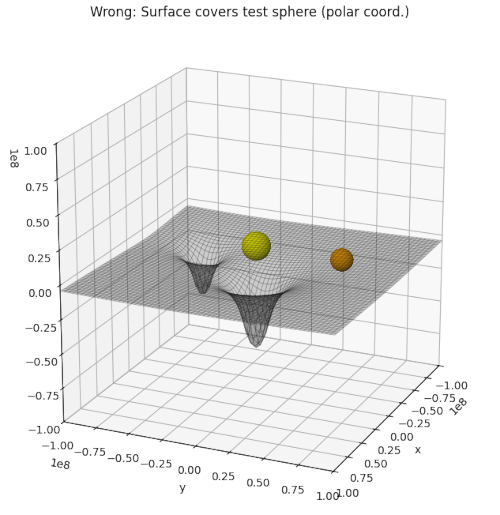
The yellow sphere with a radius of 1.0e7 is positioned at (x=0, y=0, z=0), the smaller orange sphere with radius 0.8e7 is at (x=0.40e8, y=0.8e8, z ≈ 0.25e8) – both clearly in front of the surface whose edges are below the z=0-plane. Nevertheless, Matplotlib renders the surface as if it were located in front of the spheres and thus obscuring them.
So, separate invocations of add_collection3d for different objects did not help.
S3Dlib: Correct rendering when data collections for spheres and surface are based on identical coordinate systems and get combined in one common collection object
The clue to a solution is to combine the data collections for the different objects’ surfaces (and of respective polygons) in one common collection object and render the respective overlapping polygons in one swipe with the help of “ax.add_collection3d()”. The problem is that an “addition” of the objects requires them to contain arrays of equal dimensions for coordinates given in the same coordinate system.
To achieve this with our code we set b_test=False. Among other things, this triggers the transformation of our two massive spheres “sph_b_cart” and “sph_s_cart” from polar to Cartesian coordinates. These two spheres are positioned above the minima of the gravitational potential. Afterward, the respective object data are combined to form a super collection object. Now, we get:
And this is obviously right.
Conclusion
Matplotlib has some weaknesses regarding a correct 3D rendering of objects with overlapping parts of their surfaces along the line of view. Problems occur when objects are rendered independently and added separately to a 3D axes frame. In principle, Matplotlib has a solution for a correct 3D-rendering of overlapping closed polygons. They must be rendered in one swipe using the information contained in one common “Poly3DCollection” object.
S3Dlib supports the Matplotlib user regarding the construction of elementary objects in different appropriate coordinate systems. It also offers a method for transforming between different coordinate systems, such that we later can combine the objects’ data in one super-object of the respective polygons. This then allows for a proper 3D rendering during which the occlusions along the line of view are handled correctly.
In this post we have demonstrated this for a combination of opaque spheres with a 2-dim manifold.
Links/Literature
[1] M. Castellana, 2024, “Plot solid 3D surface on top of another one”,
Post Post plot-solid-3d-surface-on-top-of-another-one/24665 at https://discourse.matplotlib.org/t/
[2] [Bug]: Multiple 3D objects are not rendered correctly #29060, https://github.com/ matplotlib/ matplotlib/ issues/29060
[3] S3Dlib documentation : https://s3dlib.org/index.html