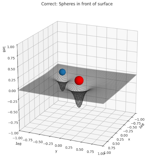
Recently, I needed a certain type of 3D-illustration for a post series about cosmology. I wanted to show a 2-dimensional manifold above a mesh grid with respective coordinate lines on the surface. In front of the surface I wanted to place some opaque spheres. Such illustrations are often used in physics to demonstrate the effect of some objects on a physical quantity – e.g. of spherical bodies on the gravitational potential or on a component of the metric tensor of space-time.
The simple problem to get a correct rendering of objects along a defined line of view upon a 3D scene posed a problem for Matplotlib’s 3D renderer for multiple objects in a 3D axis frame (created by ax = plt.axes(projection=’3d’)). The occlusion of objects was displayed wrongly for most view ports and viewing angles.
In this post, I briefly want to outline how this problem can be solved with the help of S3Dlib. As a beginner regarding the use of S3Dlib, I had to overcome some problems there, too. So, this small exercise with some options of S3Dlib might be interesting for some readers which want to use Python and Matplotlib for rendering simple 3D scenes.
The following plot shows what I wanted to achieve:
Correct rendering of two spheres in front of a surface by S3DlibContinue reading →
This post requires Javascript to display formulas!
In Machine Learning [ML] or statistics it is interesting to visualize properties of multivariate distributions by projecting them into 2- or 3-dimensional sub-spaces of the datas’ original n-dimensional variable space. The 3-dimensional aspects are not so often used because plotting is more complex and you have to fight with transparency aspects. Nevertheless a 3-dim view on data may sometimes be more instructive than the analysis of 2-dim projections. In this post we care about 3-dim data representations of tri-variate distributions X with matplotlib. And we add ellipsoids from a corresponding tri-variate normal distribution with the same covariance matrix as X.
Multivariate normal distribution and their projection into a 3-dimensional sub-space
A statistical multivariate distribution of data points is described by a so called random vectorX in an Euclidean space for the relevant variables which characterize each object of interest. Many data samples in statistics, big data or ML are (in parts) close to a so called multivariate normal distribution [MND]. One reason for this is, by the way, the “central limit theorem”. A multivariate data distribution in the ℝn can be projected orthogonally onto a 3-dimensional sub-space. Depending on the selected axes that span the sub-space you get a tri-variate distribution of data points.
Whilst analyzing a multivariate distribution you may want to visualize for which regions of variable values your projected tri-variate distributions X deviate from adapted and related theoretical tri-variate normal distributions. The relation will be given by relevant elements of the covariance matrix. Such a deviation investigation defines an application “case 1”.
Another application case, “case 2”, is the following: We may want to study a 3-variate MND, a TND, to get a better idea about the behavior of MNDs in general. In particular you may want to learn details about the relation of the TND with its orthogonal projections onto coordinate planes. Such projections give you marginal distributions in sub-spaces of 2 dimensions. The step from analyzing bi-variate to analyzing tri-variate normal distributions quite often helps to get a deeper understanding of MNDs in spaces of higher dimension and their generalized properties.
When we have a given n-dimensional multivariate random vector X (with n > 3) we get 3-dimensional data by applying an orthogonal projection operatorP on the vector data. The relatively trivial operator projects the data orthogonally into a sub-volume spanned by three selected axes of the full variable space. For a given random vector their will, of course, exist multiple such projections as there is a whole bunch of 3-dim sub-spaces for a big n. In “case 2”, however, we just create basic vectors of a 3-dim MND via a proper random generation function.
Regarding matplotlib for Python we can use a scatter-plot function to visualize the resulting data points in 3D. Typically, plots of an ideal or approximate tri-variate normal distribution [TND] will show a dense ellipsoidal core, but also a diffuse and only thinly populated outer region. To get a better impression of the spatial distribution of X relative to a TND and the orientation of the latter’s main axes it might be helpful to include ideal contour surfaces of the TND into the plots.
It is well known that the contour surfaces of multivariate normal distributions are surfaces of nested ellipsoids. On first sight it may, hower, appear difficult to combine impressions of such 2-dim hyper-surfaces with a 3-dim scatter plot. In particular: Where from do we get the main axes of the ellipsoids? And how to plot their (hyper-) surfaces?
Objective of this post
The objective of this post is to show that we can derive everything that is required
to plot general tri-variate distributions
plus ellipsoids from corresponding tri-variate normal distributions
from the covariance matrixΣ of our random vector X.
In case 2 we will just have to define such a matrix – and everything else will follow from it. In case 1 you have to first determine the (n x n)-covariance matrix of your random vector and then extract the relevant elements for the (3 x 3)-covariance matrix of the projected distribution out of it.
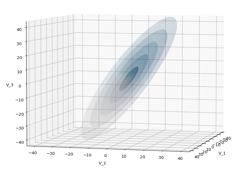
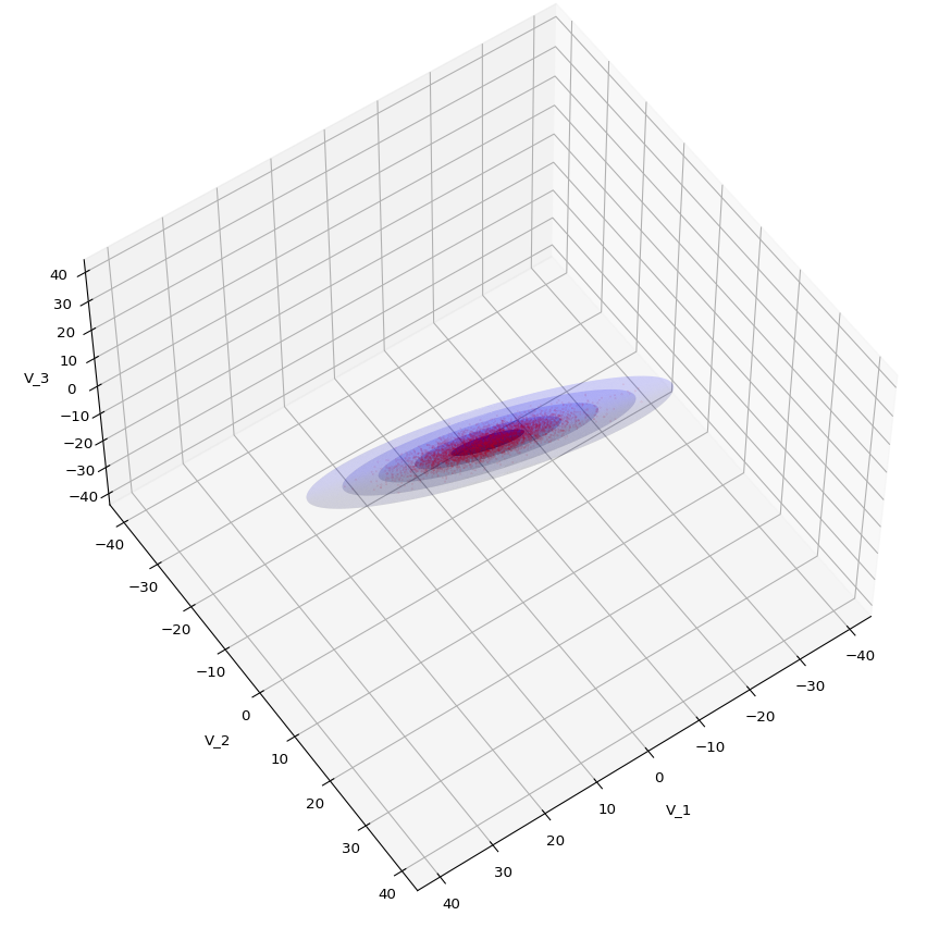
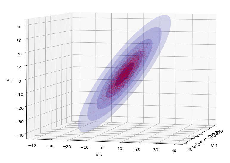
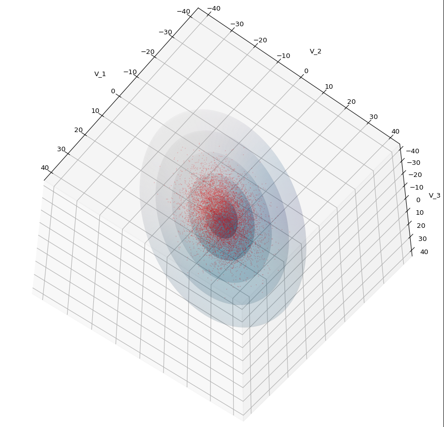
The result will be plots like the following:
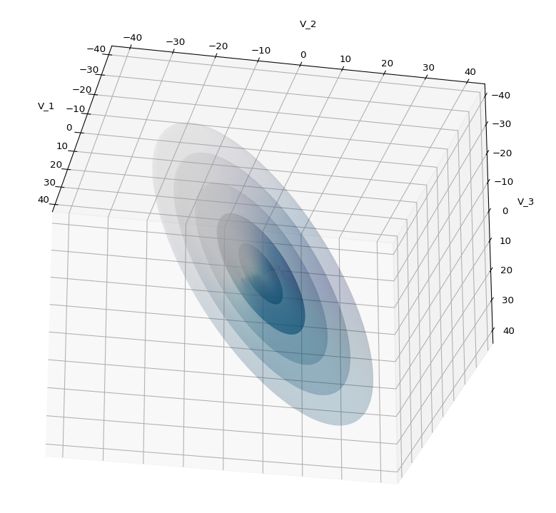
The first plot combines a scatter plot of a TND with ellipsoidal contours. The 2nd plot only shows contours for confidence levels 1 ≤ σ ≤ 5 of our ideal TND. And I did a bit of shading.
How did I get there?
The covariance matrix determines everything
The mathematical object which characterizes the properties of a MND is its covariance matrix (Σ). Note that we can determine a (n x n)-covariance matrix for any X in n dimensions. Numpy provides a function cov() that helps you with this task. The relevant elements of the full covariance matrix for orthogonal projections into a 3-dim sub-space can be extracted (or better: cut out) by applying a suitable projection operator. This is trivial: Just select the elements with the (i, i)- and (i, j)-indices corresponding to the selected axes of the sub-space. The extracted 9 elements will then form the covariance matrix of the projected tri-variate distribution.
In case 2 we just define a (3 x 3)-Σ as the starting point of our work.
Let us assume that we got the essential Σ-matrix from an analysis of our distribution data or that we, in case 2, have created it. How does a (3 x 3)-Σ relate to ellipsoidal surfaces that show the same deformation and relations of the axes’ lengths as a corresponding tri-variate normal distribution?
Creation of a MND from a standardized normal distribution
In general any n-dim MND can be constructed from a standardized multivariate distribution of independent (and consequently uncorrelated) normal distributions along each axis. I.e. from n univariate marginal distributions. Let us call the standardized multivariate distribution SMND and its random vector Z. We use the coordinate system [CS] where the coordinate axes are aligned with the main axes of the SMND as the CS in which we later also will describe our given distribution X. Furthermore the origin of the CS shall be located such that the SMND is centered. I.e. the mean vector μ of the distribution shall coincide with the CS’s origin:
\[ \pmb{\mu} \: = \: \pmb{0}
\]
In this particular CS the (probability) density function f of Z is just a product of Gaussians gj(zj) in all dimensions with a mean at the origin and standard deviations σj = 1, for all j.
With z = (z1, z2, …, zn) being a position vector of a data point in the distribution, we have:
The construction recipe for the creation of a general MND XN from Z is just the application of a (non-singular) linear transformation. I.e. we apply a (n x n)-matrix onto the position vectors of the data points in the ℝn. Let us call this matrix A. I.e. we transform the random vector Z to a new random vector XN by
Σ determines the shape of the resulting probability distribution completely. We can reconstruct an A’ which produces the same distribution by an eigendecomposition of the matrix ΣX. A’ afterward appears as a combination of a rotation and a scaling. An eigendecomposition leads in general to
D contains the eigenvalues of Σ, whereas the columns of V are the components of the eigenvectors of Σ (in the present coordinate system). V represents a rotation and D a scaling.
The required transformation matrix T, which leads from the unrotated and unscaled SMND Z to the MND XN, can be rewritten as
The 1/2 abbreviates the square root of the matrix values (i.e. of the eigenvalues). A relevant condition is that ΣX is a symmetric and positive-definite matrix. Meaning: The original A itself must not be singular!
This works in n dimensions as well as in only 3.
Creation of a trivariate normal distribution
The creation of a centered tri-variate normal distribution is easy with Python and Numpy: We just can use
np.random.multivariate_normal( mean, Σ, m )
to create m statistical data points of the distribution. Σ must of course be delivered as a (3 x 3)-matrix – and it has to be positive definite. In the following example I have used
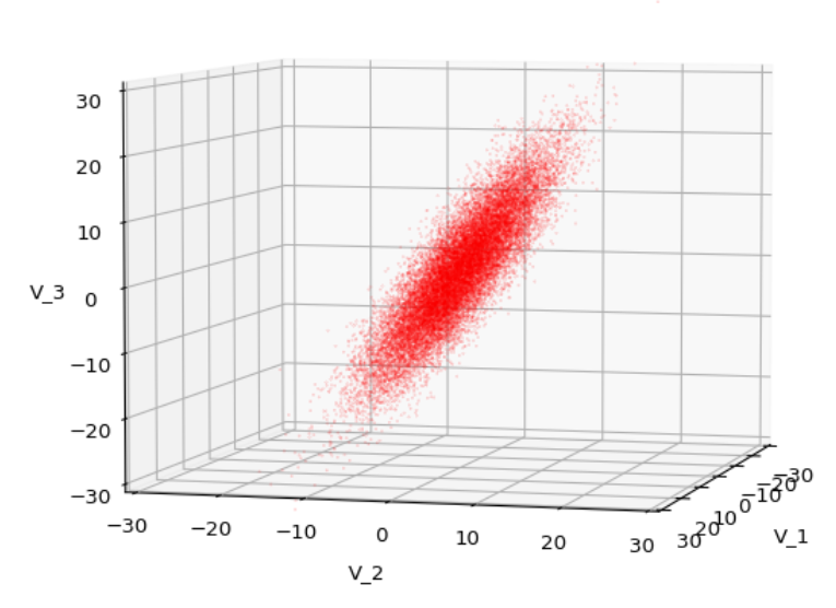
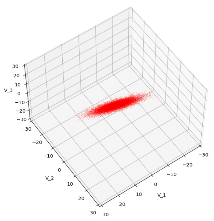
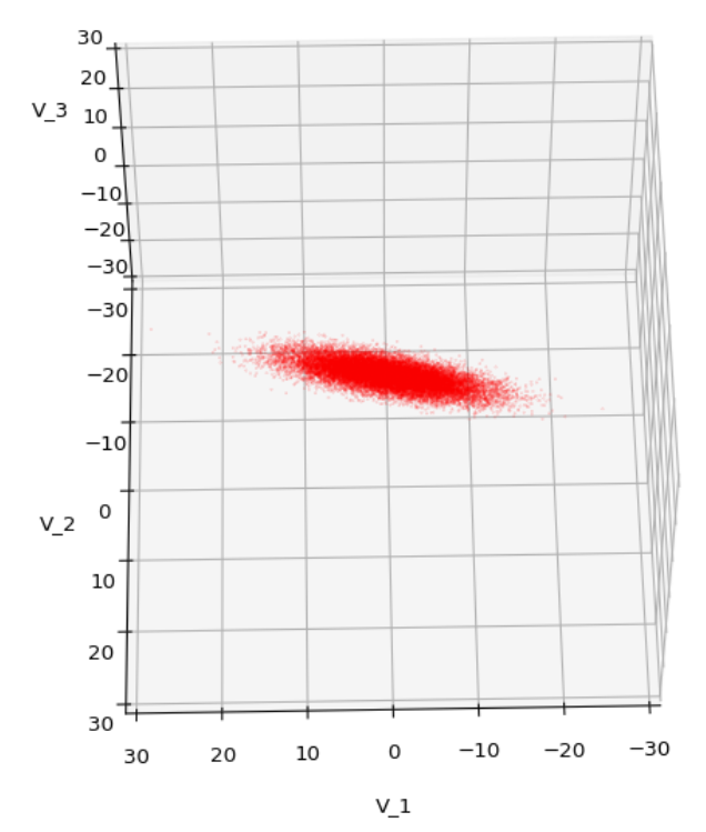
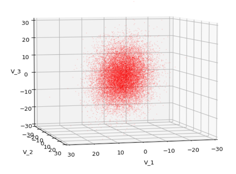
We have to feed this Σ-matrix directly into np.random.multivariate_normal(). The result with 20,000 data points looks like:
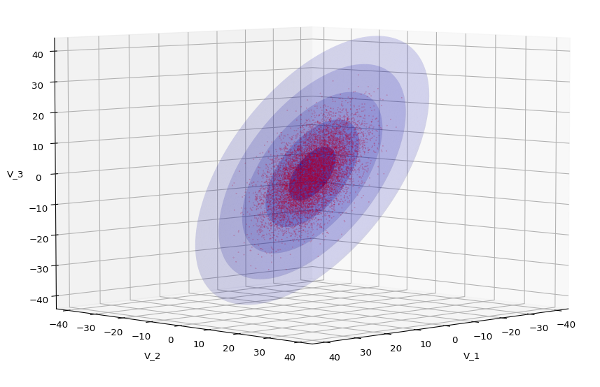
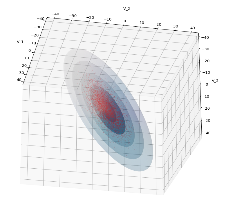
We see a dense inner core, clearly having an ellipsoidal shape. While the first image seems to indicate an overall slim ellipsoid, the second image reveals that our TND actually looks more like an extended lens with a diagonal orientation in the CS. =>
Note: When making such §D-plots we have to be careful not to make premature conclusions about the overall shape of the distribution! Projection effects may give us a wrong impression when looking from just one particular position and viewing angle onto the 3-dimensional distribution.
Create some nested transparent ellipsoidal surfaces
Especially in the outer regions the distribution looks a bit fluffy and not well defined. The reason is the density of points drops rapidly beyond a 3-σ-level. One gets the idea that a sequence of nested contour surfaces may be helpful to get a clearer image of the spatial distribution. We know already that contour surfaces of a MND are the surfaces of ellipsoids. How to get these surfaces?
The answer is rather simple: We just have to apply the mathematical recipe from above to specific data points. These data points must be located on the surface of a unit sphere (of the Z-distribution). Let us call an array with three rows for x-, y-, z-values and m columns for the amount of data points on the 3-dimensional unit sphere US. Then we need to perform the following transformation operation:
to get a valid distribution SX of points on the surface of an ellipsoid with the right orientation and relation of the main axes lengths. The surface of such an ellipsoid defines a contour surface of a TND with the covariance matrix Σ.
After the application of T to these special points we can use matplotlib’s
ax.plot_surface(x, y, z, …)
to get a continuous surface image.
To get multiple nested surfaces with growing diameters of the related ellipsoids we just have to scale (with growing and common integer factors applied to the σj-eigen-values).
Note that we must create all the surfaces transparent – otherwise we would not get a view to inner regions and other nested surfaces. See the code snippets below for more details.
SVD decomposition
We also have to get serious about numerically calculating T. I.e., we need a way to perform the “eigendecomposition”. Technically, we can use the so called “Singular Value Decomposition” [SVD] from Numpy’s linalg-module, which for symmetric matrices just becomes the eigendecomposition.
Code snippets
We can now write down some Jupyter cells with Python code to realize our SVD decomposition. I omit any functionality to project your real data into a 3-dim sub-space and to derive the covariance matrix. These are standard procedures in ML or statistics. But the following code snippets will show which libraries you need and the basic steps to create your plots. Instead of a general MND, I will create a TND for scatter plot points:
Code cell 1 – Imports
import numpy as np
import matplotlib as mpl
from matplotlib import pyplot as plt
from matplotlib.colors import ListedColormap
import matplotlib.patches as mpat
from matplotlib.patches import Ellipse
from matplotlib.colors import LightSource
Code cell 2 – Function to create points on a unit sphere
# Function to create points on unit sphere
def pts_on_unit_sphere(num=200, b_print=True):

    # Create pts on unit sphere
    u = np.linspace(0, 2 * np.pi, num)
    v = np.linspace(0, np.pi, num)

    x = np.outer(np.cos(u), np.sin(v))
    y = np.outer(np.sin(u), np.sin(v))
    z = np.outer(np.ones_like(u), np.cos(v))

    # Make array
    unit_sphere = np.stack((x, y, z), 0).reshape(3, -1)

    if b_print:
        print()
        print("Shapes of coordinate arrays : ", x.shape, y.shape, z.shape)
        print("Shape of unit sphere array : ",  unit_sphere.shape)
        print()

    return unit_sphere, x
Code cell 3 – Function to plot TND with ellipsoidal surfaces
# Function to plot a TND with supplied allipsoids based on the sam Sigma-matrix
def plot_TND_with_ellipsoids(elevation=5, azimuth=5,
                             size=12, dpi=96,
                             lim=30, dist=11,
                             X_pts_data=[],
                             li_ellipsoids=[],
                             li_alpha_ell=[],
                             b_scatter=False, b_surface=True,
                             b_shaded=False, b_common_rgb=True,
                             b_antialias=True,
                             pts_size=0.02, pts_alpha=0.8,
                             uniform_color='b', strid=1,
                             light_azim=65, light_alt=45
                            ):

    # Prepare figure
    plt.rcParams['figure.dpi'] = dpi
    fig = plt.figure(figsize=(size,size))  # Square figure
    ax = fig.add_subplot(111, projection='3d')

    # Check data
    if b_scatter:
        if len(X_pts_data) == 0:
            print("Error: No scatter points available")
            return

    if b_surface:
        if len(li_ellipsoids) == 0:
             print("Error: No ellipsoid points available")
             return
        if len(li_alpha_ell) < len(li_ellipsoids):
             print("Error: Not enough alpha values for ellipsoida")
             return
        num_ell = len(li_ellipsoids)

    # set limits on axes
    if b_surface:
        lim = lim * 1.7
    else:
        lim = lim

    # axes and labels
    ax.set_xlim(-lim, lim)
    ax.set_ylim(-lim, lim)
    ax.set_zlim(-lim, lim)
    ax.set_xlabel('V_1', labelpad=12.0)
    ax.set_ylabel('V_2', labelpad=12.0)
    ax.set_zlabel('V_3', labelpad=6.0)

    # scatter points of the MND
    if b_scatter:
        x = X_pts_data[:, 0]
        y = X_pts_data[:, 1]
        z = X_pts_data[:, 2]
        ax.scatter(x, y, z, c='r', marker='o', s=pts_size, alpha=pts_alpha)

    # ellipsoidal surfaces
    if b_surface:
        # Shaded
        if b_shaded:
            # Light source
            ls = LightSource(azdeg=light_azim, altdeg=light_alt)
            cm = plt.cm.PuBu
            li_rgb = []
            for i in range(0, num_ell):
                zz = li_ellipsoids[i][2,:]
                li_rgb.append(ls.shade(zz, cm))

            if b_common_rgb:
                for i in range(0, num_ell-1):
                    li_rgb[i] = li_rgb[num_ell-1]

            # plot the ellipsoidal surfaces
            for i in range(0, num_ell):
                ax.plot_surface(*li_ellipsoids[i],
                                rstride=strid, cstride=strid,
                                linewidth=0, antialiased=b_antialias,
                                facecolors=li_rgb[i],
                                alpha=li_alpha_ell[i]
                               )
        # just uniform color
        else:
            print("here")
            #ax.plot_surface(*ellipsoid, rstride=2, cstride=2, color='b', alpha=0.2)
            for i in range(0, num_ell):
                ax.plot_surface(*li_ellipsoids[i],
                                rstride=strid, cstride=strid,
                                color=uniform_color, alpha=li_alpha_ell[i])

    ax.view_init(elev=elevation, azim=azimuth)
    ax.dist = dist
    return
Some hints: The scatter data from the distribution X (or XN) must be provided as a Numpy array. The TND-ellipsoids and the respective alpha values must be provided as Python lists. Also the size and the alpha-values for the scatter points can be controlled. Reducing both can be helpful to get a glimpse also on ellipsoids within the relative dense core of the TND.
Some parameters as “elevation”, “azimuth”, “dist” help to control the viewing perspective. You can switch showing of the scatter data as well as ellipsoidal surfaces and their shading on and off by the Boolean parameters.
There are a lot of parameters to control a primitive kind of shading. You find the relevant information in the online documentation of matplotlib. The “strid” (stride) parameter should be set to 1 or 2. For slower CPUs one can also take higher values. One has to define a light-source and a rgb-value range for the z-values. You are free to use a different color-map instead of PuBu and make that a parameter, too.
Code cell 4 – Covariance matrix, SVD decomposition and derivation of the T-matrix
b_print = True

# Covariance matrix
cov1 = [[31.0, -4, 5], [-4, 26, 44], [5, 44, 85]]
cov = np.array(cov1)

# SVD Decomposition
U, S, Vt = np.linalg.svd(cov, full_matrices=True)
S_sqrt = np.sqrt(S)

# get the trafo matrix T = U*SQRT(S)
T = U * S_sqrt

# Print some info
if b_print:
    print("Shape U: ", U.shape, " :: Shape S: ", S.shape)
    print(" S      : ", S)
    print(" S_sqrt : ", S_sqrt)
    print()
    print(" U :\n", U)
    print(" T :\n", T)
Code cell 5 – Transformation of points on a unit sphere
# Transform pts from unit sphere onto surface of ellipsoids
# ~~~~~~~~~~~~~~~~~~~~~~~~~~~~~~~
b_print = True
num = 200
unit_sphere, xs = pts_on_unit_sphere(num=num)

# Apply transformation on data of unit sphere
ell_transf = T @ unit_sphere
# li_fact = [2.5, 3.5, 4.5, 5.5, 6.5]
li_fact = [1.0, 2.0, 3.0, 4.0, 5.0]
num_ell = len(li_fact)
li_ellipsoids = []
for i in range(0, num_ell):
    li_ellipsoids.append(li_fact[i] * ell_transf.reshape(3, *xs.shape))

if b_print:
    print("Shape ell_transf  : ", ell_transf.shape)
    print("Shape ell_transf0 : ", li_ellipsoids[0].shape)
Code cell 6 – TND data point creation and plotting
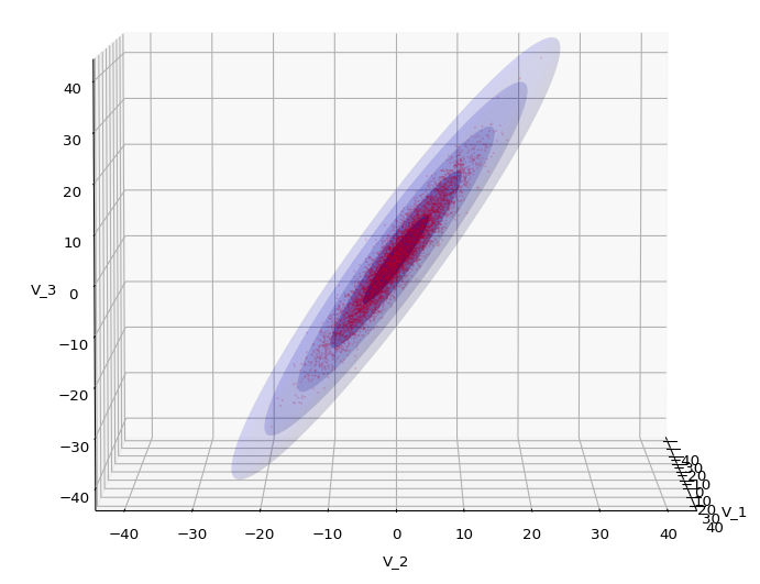
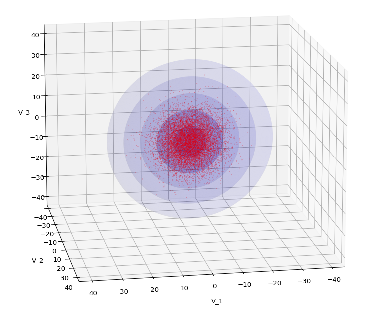
Let us play a bit around. The ellipsoidal contours are for σ = 1, 2, 3 ,4, 5. First we look at the data distribution from above. The ellipsoidal contours are for σ = 1, 2, 3 ,4, 5. We must reduce the size and alpha of the scatter points to 0.01 and 0.45, respectively, to still get an indication of the innermost ellipsoid of σ = 1. I used 8000 scatter points. The following plots show the same from different side perspectives – with and without shading and adapted alpha-values and number values for the scatter points
.
Yoo see: How a TND appears depends strongly on the viewing position. From some positions the distribution’s projection of the viewer’s background plane may even appear spherical. But on the other side it is remarkable how well the projection onto a background plane keeps up the ellipses of the projected outermost borders of the contour surfaces (of the ellipsoids for confidence levels). This is a dominant feature of MNDs in general.
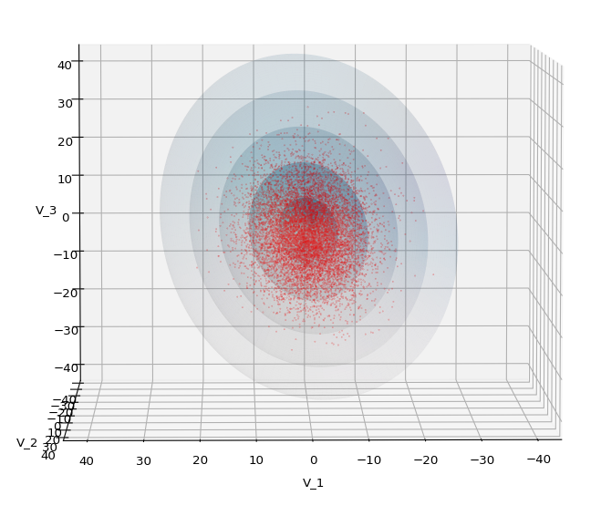
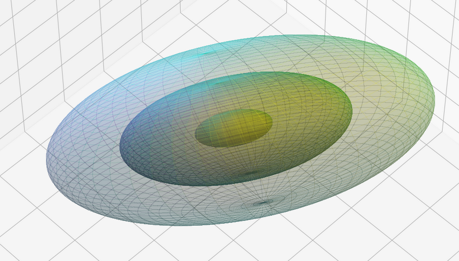
A last hint: To get a more volumetric impression it is required to both work with the position of the lightsource, the alpha-values and the colormap. In addition turning off ant-aliasing and setting the stride to something like 5 may be very helpful, too. The next image was done for an ellipsoid with slightly different extensions, only 3 ellipsoids and stride=5:
Conclusion
In this blog I have shown that we can display a tri-variate (normal) distribution, stemming from a construction of a standardized normal distribution or from a projection of some real data distribution, in 3D with the help of Numpy and matplotlib. As soon as we know the covariance matrix of our distribution we can add transparent surfaces of ellipsoids to our plots. These are constructed via a linear transformation of points on a unit sphere. The transformation matrix can be derived from an eigendecomposition of the covariance matrix.
The added ellipsoids help to better understand the shape and orientation of the tri-variate distribution. But plots from different viewing angles are required.
During some work for a ML project on a large text corpus I needed to extend a personally used reference vocabulary by some complex ad unusual German compounds and very branch specific technical terms. I kept my vocabulary data in a Pandas dataframe. Each “word” there had some additional information associated with it in some extra columns of the dataframe – as e.g. the length of a word or a stem or a list of constituting tri-char-grams. I was looking for a fast method to extend the dataframe in a quick procedure with a list of hundreds or thousands of new words.
I tried the df.append() method first and got disappointed with its rather bad performance. I also experimented with the incorporation of some lists or dictionaries. In the end a procedure based on csv-data was the by far most convenient and fastest approach. I list up the basic steps below.
In my case I used the lower case character version of the vocabulary words as an index of the dataframe. This is a very natural step. It requires some small intermediate column copies in the step sequence below, which may not be necessary for other use-cases. For the sake of completeness the following list contains many steps which have to be performed only once and which later on are superfluous for a routine workflow.
Step1: Collect your extension data, i.e. a huge bunch of words, in a Libreoffice Calc-file in ods-format or (if you absolutely must) in an MS Excel-file. One of the columns of your datasheet should contain data which you later want to use as a (unique) index of your dataframe – in my case a column “lower” (containing the low letter representation of a word).
Step 2: Avoid any operations for creating additional column information which you later can create by Python functions working on information already contained in some dataframe columns. Fill in dummy values into respective columns. (Or control the filling of a dataframe with special data during the data import below)
Step 3: Create a CSV-File containing the collected extension data with all required field information in columns which correspond to respective columns of the dataframe to be extended.
Step 4:Create a backup copy of your original dataframe which you want to extend. Just as a precaution ….
Step 5: Copy the contents of the index of your existing dataframe to a specific dataframe column consistent with step 1. In my case I copied the words’ lower case version into a new data column “lower”.
Step 6: Delete the existing index of the original dataframe and create a new basic integer based index.
Step 7: Import the CSV-file into a new and separate intermediate Pandas dataframe with the help of the method pd.read_csv(). Map the data columns and the data formats properly by supplying respective (list-like) information to the parameter list of read_csv(). Control the filling of possibly empty row-fields. Check for fields containing “null” as string and handle these by the parameter “na_filter” if possible (in my case by “na_filter=False”)
Step 8: Work on the freshly created dataframe and create required information in special columns by applying row-specific Python operations with a function and the df.apply()-method. For the sake of performance: Watch out for naturally vectorizable operations whilst doing so and separate them from other operations, if possible.
Step 9: Check for completeness of all information in
your intermediate dataframe. verify that the column structure matches the columns of the original dataframe to be extend.
Step 10: Concatenate the original Pandas dataframe (for your vocabulary) with the new dataframe containing the extension data by using the df.concat() or (simpler) by df.append() methods.
Step 11: Drop the index in the extended dataframe by the method pd.reset_index(). Afterward recreate a new index by pd.set_index() and using a special column containing the data – in my case the column “lower”
Step 12: Check the new index for uniqueness – if required.
Step 13: If uniqueness is not given but required: Apply df = df[~df.index.duplicated(keep=’first’)] to keep only the first occurrence of rows for identical indices. But be careful and verify that this operation really fits your needs.
Step 14: Resort your index (and extended dataframe) if necessary by applying df.sort_index(inplace=True)
Some steps in the list above are of course specific for a dataframe with a vocabulary. But the general scheme should also be applicable for other cases.
From the description you have certainly realized which steps must only be performed once in the beginning to establish a much shorter standard pipeline for dataframe extensions. Some operations regarding the index-recreation and re-sorting can also be automatized by some simple Python function.
In the last posts of this mini-series we have studied if and how we can use three 3-char-grams at defined positions of a string token to identify matching words in a reference vocabulary. We have seen that we should choose some distance between the char-grams and that we should use the words length information to keep the list of possible hits small.
Such a search may be interesting if there is only fragmented information available about some words of a text or if one cannot trust the whole token to be written correctly. There may be other applications. Note: This has so far nothing to do with text analysis based on machine learning procedures. I would put the whole topic more in the field of text preparation or text rebuilding. But, I think that one can combine our simple identification of fitting words by 3-char-grams with ML-methods which evaluate the similarity or distance of a (possibly misspelled) token with vocabulary words: When we get a long hit-list we could invoke ML-methods to to determine the best fitting word.
We saw that we can do a 100,000 search runs with 3-char-grams on a decent vocabulary of around 2 million words in a Pandas dataframe below a 1.3 minutes on one CPU core of an older PC. In this concluding article I want to look a bit at the idea of multiprocessing the search with up to 4 CPU cores.
Points to take into account when using multiprocessing – do not expect too much
Pandas normally just involves one CPU core to do its job. And not all operations on a Pandas dataframe may be well suited for multiprocessing. Readers who have followed the code fragments in this series so far will probably and rightly assume that there is indeed a chance for reasonably separating our search process for words or at least major parts of it.
But even then – there is always some overhead to expect from splitting a Pandas dataframe into segments (or “partitions”) for a separate operations on different CPU cores. Overhead is also expected from the task to correctly to combine the particular results from the different processor cores to a data unity (here: dataframe) again at the end of a multiprocessed run.
A bottleneck for multiprocessing may also arise if multiple processes have to access certain distinct objects in memory at the same time. In our case we this point is to be expected for the access of and search within distinct sub-dataframes of the vocabulary containing words of a specific length.
Due to overhead and bottlenecks we do not expect that a certain problem scales directly and linearly with the number of CPU cores. Another point is that although the Linux OS may recognize a hyperthreading physical core of an Intel processor as two cores – but it may not be able to use such virtual cores in a given context as if they were real separate physical cores.
Code to invoke multiple processor cores
In this article I just use the standard Python “multiprocessing” module. (I did not test Ray yet – as a first trial gave me trouble in some preparing code-segments of my Jupyter notebooks. I did not have time to solve the problems there.)
Following some advice on the Internet I handled parallelization in the following way:
import multiprocessing
from multiprocessing import cpu_count, Pool

#cores = cpu_count() # Number of physical CPU cores on your system
cores = 4
partitions = cores # But actually you can define as many partitions as you want

def parallelize(data, func):
    data_split = np.array_split(data, partitions)
    pool = Pool(cores)
    data = pd.concat(pool.map(func, data_split), copy=False)
    pool.close()
    pool.join()
    return data
The basic function, corresponding to the parameter “func” of function “parallelize”, which shall be executed in our case is structurally well known from the last posts of this article series:
We perform a search via
putting conditions on columns (of the vocabulary-dataframe) containing 3-char-grams at different positions. The search is done on sub-dataframes of the vocabulary containing only words with a given length. The respective addresses are controlled by a Python dictionary “d_df”; see the last post for its creation. We then build a list of indices of fitting words. The dataframe containing the test tokens – in our case a random selection of real vocabulary words – will be called “dfw” inside the function “func() => getlen()” (see below). To understand the code you should be aware of the fact that the original dataframe is split into (4) partitions.
We only return the length of the list of hits and not the list of indices for each token itself.
# Function for parallelized operation
# ~~~~~~~~~~~~~~~~~~~~~~~~~~~~~~~~~~~~
def getlen(dfw):
    # Note 1: The dfw passed is a segment ("partition") of the original dataframe
    # Note 2: We use a dict d_lilen which was defined outside
    #         and is under the control of the parallelization manager

    num_rows = len(dfw)
    for i in range(0, num_rows):
        len_w = dfw.iat[i,0]
        idx = dfw.iat[i,33]

        df_name = "df_" + str(len_w)
        df_ = d_df[df_name]

        j_m = math.floor(len_w/2)+1
        j_l = 2
        j_r = len_w -1
        col_l = 'gram_' + str(j_l)
        col_m = 'gram_' + str(j_m)
        col_r = 'gram_' + str(j_r)
        val_l = dfw.iat[i, j_l+2]
        val_m = dfw.iat[i, j_m+2]
        val_r = dfw.iat[i, j_r+2]
        li_ind = df_.index[   (df_[col_r]==val_r)
                            & (df_[col_m]==val_m)
                            & (df_[col_l]==val_l)
                            ]
        d_lilen[idx] = len(li_ind)

    # The dataframe must be returned - otherwise it will not be concatenated after parallelization
    return dfw
While the processes work on different segments of our input dataframe we write results to a Python dictionary “d_lilen” which is under the control of the “parallelization manager” (see below). A dictionary is appropriate as we might otherwise loose control over the dataframe-indices during the following processes.
A reduced dataframe containing randomly selected “tokens”
To make things a bit easier we first create a “token”-dataframe “dfw_shorter3” based on a random selection of 100,000 indices from a dataframe containing long vocabulary words (length ≥ 10). We can derive it from our reference vocabulary. I have called the latter dataframe “dfw_short3” in the last post (because we use three 3-char-grams for longer tokens). “dfw_short3” contains all words of our vocabulary with a length of “10 ≤ length ≤ 30”.
# Prepare a sub-dataframe for of the random 100,000 words
# ******************************
num_w = 100000
len_dfw = len(dfw_short3)
# select a 100,000 random rows
random.seed()
# Note: random.sample does not repeat values
li_ind_p_w = random.sample(range(0, len_dfw), num_w)
len_li_p_w = len(li_ind_p_w)
dfw_shorter3 = dfw_short3.iloc[li_ind_p_w, :].copy()
dfw_shorter3['lx'] = 0
dfw_shorter3['idx'] = dfw_shorter3.index
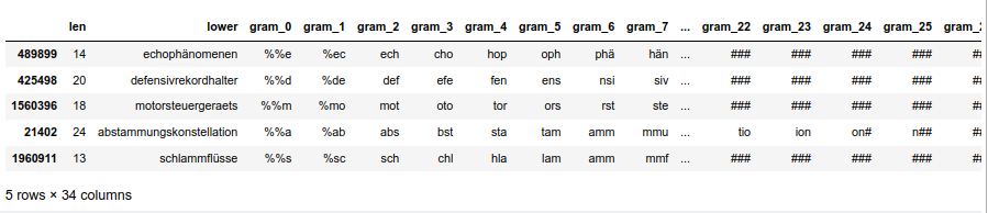
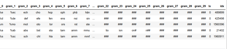
dfw_shorter3.head(5)
The resulting dataframe “dfw_shorter3” looks like :
nYou see that the index varies randomly and is not in ascending order! This is the reason why we must pick up the index-information during our parallelized operations!
Code for executing parallelized run
The following code enforces a parallelized execution:
My readers know about this effect already from ML experiments with CUDA and libcublas:
As long a s we use physical processor cores we see substantial improvement, beyond that no real gain in performance is observed on hyperthreading CPUs.
Compared to a run with just one CPU core we seem to gain a factor of almost 3 by parallelization. But, actually, this is no fair comparison: My readers have certainly seen that the CPU-time for the run with one CPU-Core is significantly slower than comparable runs which I described in my last post. At that time we found a cpu-time of around 75 secs, only. So, we have a basic deficit of about 15 secs – without real parallelization!
Overhead and RAM consumption of multiprocessing
Why does run with just one CPU core take so long time? Is it functional overhead for organizing and controlling multiprocessing – which may occur despite using just one core and just one “partition” of the dataframe (i.e. the full dataframe)? Well, we can test this easily by reconstructing the runs of my last post a bit:
# Reformulate Run just for cpu-time comparisons
# **********************************************
b_test = True

# Function
# ~~~~~~~~~~~~~~~~~~~~~~~~~~~~~~~~~~~~
def getleng(dfw, d_lileng):
    # Note 1: The dfw passed is a segment of the original dataframe
    # Note 2: We use a list l_lilen which was outside defined
    #         and is under the control of the prallelization manager

    num_rows = len(dfw)
    #print(num_rows)
    for i in range(0, num_rows):
        len_w = dfw.iat[i,0]
        idx = dfw.iat[i,33]

        df_name = "df_" + str(len_w)
        df_ = d_df[df_name]

        j_m = math.floor(len_w/2)+1
        j_l = 2
        j_r = len_w -1
        col_l = 'gram_' + str(j_l)
        col_m = 'gram_' + str(j_m)
        col_r = 'gram_' + str(j_r)
        val_l = dfw.iat[i, j_l+2]
        val_m = dfw.iat[i, j_m+2]
        val_r = dfw.iat[i, j_r+2]
        li_ind = df_.index[   (df_[col_r]==val_r)
                            & (df_[col_m]==val_m)
                            & (df_[col_l]==val_l)
                            ]
        leng = len(li_ind)
        d_lileng[idx] = leng

    return d_lileng


if b_test:
    num_w = 100000
    len_dfw = len(dfw_short3)

    # select a 100,000 random rows
    random.seed()
    # Note: random.sample does not repeat values
    li_ind_p_w = random.sample(range(0, len_dfw), num_w)
    len_li_p_w = len(li_ind_p_w)

    dfw_shortx = dfw_short3.iloc[li_ind_p_
w, :].copy()
    dfw_shortx['lx']  = 0
    dfw_shortx['idx'] = dfw_shortx.index

    d_lileng = {} #

    v_start_time = time.perf_counter()
    d_lileng = getleng(dfw_shortx, d_lileng)
    v_end_time = time.perf_counter()
    cpu_time   = v_end_time - v_start_time
    print("cpu : ", cpu_time)
    print(len(d_lileng))
    mean_length = sum(d_lileng.values()) / len(d_lileng)
    print(mean_length)

    dfw_shortx.head(3)
How long does such a run take?
cpu :  77.96989408900026
100000
1.25666
Just 78 secs! This is pretty close to the number of 75 secs we got in our last post’s efforts! So, we see that turning to multiprocessing leads to significant functional overhead! The gain in performance, therefore, is less than the factor 3 observed above:
We (only) get a gain in performance by a factor of roughly 2.5 – when using 4 physical CPU cores.
I admit that I have no broad or detailed experience with Python multiprocessing. So, if somebody sees a problem in my code, please, send me a mail.
RAM is not released completely
Another negative side effect was the use of RAM in my case. Whereas we just get 2.2 GB RAM consumption with all required steps and copying parts of the loaded dataframe with all 3-char-grams in the above test run without multiprocessing, I saw a monstrous rise in memory during the parallelized runs:
Starting from a level of 2.4 GB, memory rose to 12.5 GB during the run and then fell back to 4.5 GB. So, there are copying processes and memory is not completely released again in the end – despite having all and everything encapsulated in functions. Repeating the multiprocessed runs even lead to a systematic increase in memory by about 150 MB per run.
So, when working with the “multiprocessing module” and big Pandas dataframes you should be a bit careful about the actual RAM consumption during the runs.
Conclusion
This series about finding words in a vocabulary by using two or three 3-char-grams may have appeared a bit “academical” – as one of my readers told me. Why the hell should someone use only a few 3-char-grams to identify words?
Well, I have tried to give some answers to this question: Under certain conditions you may only have fragments of words available; think of text transcribed from a recorded, but distorted communication with Skype or think of physically damaged written text documents. A similar situation may occur when you cannot trust a written string token to be a correctly written word – due to misspelling or other reasons (bad OCR SW or bad document conditions for scans combined with OCR).
In addition: character-grams are actually used as a basis for multiple ML methods for text-analysis tasks, e.g. in Facebook’s Fasttext. They give a solid base for an embedded word vector space which can help to find and measure similarities between correctly written words, but also between correctly written words and fantasy words or misspelled words. Looking a bit at the question of how much a few 3-char-grams help to identify a word is helpful to understand their power in other contexts, too.
We have seen that only three 3-char-grams can identify matching words quite well – even if the words are long words (up to 30 characters). The list of matching words can be kept surprisingly small if and when
we use available or reasonable length information about the words we want to find,
we define positions for the 3-char-grams inside the words,
we put some positional distance between the location of the chosen 3-char-grams inside the words.
For a 100,000 random cases with correctly written 3-char-grams the average length of the hit list was below 2 – if the distance between the 3-char-grams was
reasonably large compared to the token-length. Similar results were found for using only two 3-char-grams for short words.
We have also covered some very practical aspects regarding search operation on relatively big Pandas dataframes :
The CPU-time for identifying words in a Pandas dataframe by using 3-char-grams is reasonably small to allow for experiments with around 100,000 tokens even on PCs within minutes or quarters of an hour – but it does not take hours. As using 3-char-grams corresponds to putting conditions on two or three columns of a dataframe this result can be generalized to other similar problems with string comparisons on dataframe columns.
The basic RAM consumption of dataframes containing up to fifty-five 3-char-grams per word can be efficiently controlled by using the dtype “category” for the respective columns.
Regarding cpu-time we saw that working with many searches may get a performance boost by a factor well above 2 by using simple multiprocessing techniques based on Python’s “multiprocessing” module. However, this comes with an unpleasant side effect of enormous RAM consumption – at least temporarily.
I hope you had some fun with this series of posts. In a forthcoming series I will apply these results to the task of error correction. Stay tuned.
Whilst preparing text data for ML we sometimes are confronted with a large amount of separate text-files organized in a directory hierarchy. In the last article in this category
I have shown how we “walk” through such a directory tree of files with the help of Python and os.walk(). We can for example use os.walk() procedure to eliminate unwanted files in the tree.
As an example I discussed a collection of around 200.000 scanned paper pages with typewriter text; the collection contained jpg-files and related OCR-based txt-files. With os.walk() I could easily get rid of the jpg-files.
A subsequent task which awaited me regarding my special text collection was the elimination of those text-files which, with a relatively high probability, were not written in German language. To solve such a problem with Python one needs a module that guesses the language of a given text correctly – in my case despite scanning and OCR errors. In this article I discuss the application of two methods – one based on the standard Python “langdetect” module and the other one based on a special variant of Facebook’s “fastText”-algorithm. The latter is by far the faster approach – which is of relevance given the relatively big number of files to analyze.
“langdetect” and its “detect()”-function
To get the “langdetect”-module import it into your virtual Python environment via “pip install langdetect“. To test its functionality just present a written text in French and another one in German from respective txt-files to the “detect()”-function of this module – like e.g. in the following Jupyter cell:
from langdetect import detect
import os
import time

ftxt1 = open('/py/projects/CA22/catch22/0034_010.txt', 'r').read()
print(detect(ftxt1))
ftxt2 = open('/py/projects/CA22/catch22/0388_001.txt', 'r').read()
print(detect(ftxt2))
In my test case this gave the result:
fr
de
So, detect() is pretty easy to use.
What about the performance of langdetect.detect()?
Let us look at the performance. For this I just ran os.walk() over the directory tree of my collection and printed out some information for all files not being of German language.
dir_path = "/py/projects/CA22/catch22/"

# use os.walk to recursively run through the directory tree
v_start_time = time.perf_counter()

n = 0
m = 0
for (dirname, subdirs, filesdir) in os.walk(dir_path):
    subdirs.sort()
    print('[' + dirname + ']')
    for filename in filesdir:
        filepath = os.path.join(dirname, filename)
        #print(filepath)
        ftext = open(filepath, 'r').read()
        lang = detect(ftext)
        if lang != 'de':
            print(filepath, ' ', lang)
            m += 1
        n += 1
    if n > 9999:
        break

v_end_time = time.perf_counter()
print("Total CPU time ", v_end_time - v_start_time)

print("num of files checked: ", n)
print("num of non German files: ", m)
Resulting numbers were:
Total CPU time  72.65049991299747
num of files checked:  10033
num of non German files:  1465
Well, printing in a browser to a Jupyter cell takes some time itself. However, we shall see that this aspect is not really relevant in this example. (The situation would be different if we had to switch contexts between GPU operations and CPU operations whilst printing in real ML applications run on a GPU, primarily.)
In addition we are only interested in relative (CPU) performance when comparing the number later to the result of fastText.
I measured 74 secs for a standard hard disk (no SSD) with printing – observing that everything just ran on one core of the CPU. Without printing the run required 72 secs. All measured with disc caching active and taking an average of three runs on cached data.
So, for my whole collection of 200.000 txt-files I would have to wait more than 25 minutes – even if the files had been opened, read and cached previously. Deleting the files form the disk would cost a bit of extra time in addition.
Without caching – i.e. for an original run I would probably have to wait for around 3 hrs. langdetect.detect() is somewhat slow.
Besides supporting a variety of real ML-tasks, fastText also offers a language detection functionality. And a Python is supported, too:
In your virtual Python environment just use “pip install fasttext”. In addition on a Linux CLI download a pretrained model for language detection, e.g. as with wget:
FastText for language detection can be used together with os.walk() as follows:
import fasttext
PRETRAINED_MODEL_PATH = '/py/projects/fasttext/lid.176.bin'
model = fasttext.load_model(PRETRAINED_MODEL_PATH)

dir_path = "/py/projects/CA22/catch22/"

# use os.walk to recursively run through the directory tree
v_start_time = time.perf_counter()

n = 0
m = 0
for (dirname, subdirs, filesdir) in os.walk(dir_path):
    subdirs.sort()
    #print('[' + dirname + ']')
    for filename in filesdir:
        filepath = os.path.join(dirname, filename)
        #print(filepath)
        ftext = open(filepath, 'r').read()
        ftext = ftext.replace("\n", " ")
        tupel_lang = model.predict(ftext)
        #print(tupel_lang)
        lang = tupel_lang[0][0][-2:]
        #print(lang)
        if lang != 'de':
            #print(filepath, ' ', lang)
            m += 1
        n += 1
    if n > 9999:
        break

v_end_time = time.perf_counter()
print("Total CPU time ", v_end_time - v_start_time)
print("num of files checked: ", n)
print("num of non German files: ", m)
Result numbers:
Total CPU time  1.895524049999949
num of files checked:  10033
num of non German files:  1355
Regarding performance fastText is almost by a factor of 38 faster than langdetect.detect() !
Eliminating non-German-files from the collection of 208.000 files took only 42 secs – once the files had been cached. An original delete run without caching took around 320 secs – which is still much faster than a detect()-run on cached data. As said on an (older) HD. This is very acceptable. SSDs would give us an even better performance.
Accuracy of the language detection
The reader certainly has noticed that the number of non-German files detected by fastText is somewhat smaller than what langdetect.detect() gave me. That there is a discrepancy is no wonder: Some of the text files are filled with so many scan and OCR errors that even a human
would have problems to detect the original language. I just checked 10 of the files where the different methods showed a discrepancy for the guessed language. In all of these 10 cases the guess of fastText was better.
Conclusion
Although I am not a friend of Facebook they have produced something really useful with their fastText algorithm. Regarding language detection fastText provides a really convincing super-fast and reliable method to guess the main language used in text pieces. It supports Python environments and allows the analysis of a huge amount of text files even on a PC.