I use email servers based on Postfix (smtp), Cyrus (imap) in combination with an LDAP server for authentication purposes and fetchmail to access external mail provider services. Both the mail servers and the LDAP server are virtualized guests on KVM host servers with LUKS-encrypted disks/partitions. Due to a series of security measures to become compliant to DSGVO and EU-GDPR based customer contracts the whole setup is relatively complicated. However, authentication for mail clients to the different servers is of central importance. Communication of each mail server to the LDAP server is performed via an TLS connection and SSSD. The mail client systems access the mail servers via TLS; login to the client systems partially also depends on LDAP.
Whenever a full upgrade of the server is required I, therefore, first test it on copies of the KVM host installation and each KVM instance. (The “dd” command is of good service during these tests.) One experiences some unwelcome surprises from time to time – and then you may need a quick restauration of a workings system.
When I switched everything to Opensuse Leap 15.1 some days ago I stumbled once again across small problems. It is interesting that one of the problems had to do with SSSD – again.
Previous problems with SSSD during upgrades to Opensuse Leap 15.0
Some time ago 1 described a problem with PAM control files for imap and smtp services on the mail server when I upgraded to Leap 15.0. See: Mail-server-upgrade to Opensuse Leap 15 – and some hours with authentication trouble
The PAM files included directives for SSSD. The file were unfortunately replaced (without backups) during upgrade from OS 42.3 to Leap 15.0. This hampered all authentication of mail clients via authentication requests from the imap and smtp services to the LDAP system. The cause of the resulting problems at the side of the email clients, namely authetication trouble, was not easy to identify.
New SSSD problem during upgrades to Opensuse Leap 15.1
This time I ran once again into authentication trouble – and suspected some mess with the PAM files again. Yet, this was not the case – the PAM files were all intact and correct. (SuSE learns!) However, after an hour of testing I saw that the SSSD service did not what it should. Checking the status of the service with “systemctl status sssd.service” I got a final status line saying “Backend is offline”.
What did this mean? I had no real clue. You naturally assume that LDAP would be my backend in my server configuration; this is reflected in the file /etc/sssd/sssd.conf:
I checked – the LDAP service was active in its KVM machine. Of course, NSS must also be working for SSSD to become functional. No problem there. I checked whether the LDAP service could be reached through the firewalls of the different KVM instances and their hosts. Yes, this worked, too. So, what the hack was wrong?
Eventually, I found some interesting contribution in a Fedora mailing list: See here. What if the problem had its origin really in some systemd glitch? Wouldn’t be the first time.
So, I first made a copy of the original file “/usr/lib/systemd/system/sssd.service” and after that tried a modification of the original file linked by “sss.service” in “/etc/systemd/system/multi-user.target.wants”. I simply added a line “After=network.service” to guarantee a full network setup before sssd was started.
[Unit]
Description=System Security Services Daemon
# SSSD must be running before we permit user sessions
Before=systemd-user-sessions.service nss-user-lookup.target
Wants=nss-user-lookup.target
After=network.service

[Service]
Environment=DEBUG_LOGGER=--logger=files
EnvironmentFile=-/etc/sysconfig/sssd
ExecStart=/usr/sbin/sssd -i ${DEBUG_LOGGER}
Type=notify
NotifyAccess=main
PIDFile=/var/run/sssd.pid

[Install]
WantedBy=multi-user.target
And guess what? This was successful! The reason being that at the point in time when the sssd.service starts name resolution (i.e. the evaluation of resolv.conf and access to DNS-servers ) may not yet be guaranteed!
Hint:
Note that there may be multiple reasons for such a delay; one you could think of is a firewall which is started at some point and requires time to establish all rules. Your server may not get access to any of the defined DNS-servers up to the point where the firewalls rules are working. Then, depending on when exactly you start your firewall service, you may have to use a different “After”-rule than mine.
Important point:
You should not permanently change the files in “/usr/lib/systemd”. So, after such a test as described you should restore the original systemd file for a specific service in “/usr/lib/systemd/system/” with all its attributes! The correct mechanism to add modifications to systemd service configuration files is e.g. described here “askubuntu.com : how-do-i-override-or-configure-systemd-services“.
So, in my case we need to execute “systemctl edit sssd” on the command line and then (in the editor window) add the lines
[Unit]
After=network.service
This leads to the creation of a directory “/etc/systemd/system/sssd.service” with a file “override.conf” which contains the required entries for service startup modification.
An additional problem with clamd – timeout during the start of the clamd service
One of my anti-virus engines integrated with amavis is clamav. More precisely the daemon based variant, i.e. the “clamd” service. However, when I tested amavis for mail scanning I saw that it used to job instances of “clamscan” instead of “clamdscan”. The impact of Amavis’ using two parallel clamscan threads was an almost 100% CPU utilization for some time.
It took me a while to find out what the cause of this problem was: clamd requires time to start up. And due to whatever reasons this time is now a bit bigger on my mail system than the standard timeout of 90 secs systemd provides. This can be compensated by “systemctl edit sssd” and adding lines as
[Service]
TimeoutSec=3min
After this change clamd ran again as usual. Note however that clamav does not provide sufficient protection on professional mail servers, especially when your email clients are based on a Windows installations. Then you need at least one more advanced (and probably costly) antivirus solution.
It is very seldom that you are confronted with a HTTP status message of type 406 “Not acceptable”. However, this happened yesterday to a customer who uses a renowned hosting provider (in Norway) to publish his web-sites. The customer uses his own WordPress installation on hosted web-servers. His favorite browser is Firefox on a Win 10 desktop system. A week ago he could work without any restrictions. Then suddenly everything changed.
Access to website and WP admin interface broken due to security measures of the provider
At some point in time during last week the hosting-provider changed his security policies on his (Norwegian) Apache servers. The provider seems to have at least changed settings of the “mod_security” module – and thereby started to eliminate old browsers by some rules. (Maybe they even introduced the use of the mod_security module for the first time ?). To implement mod-security with a reasonable set of rules basically is a good measure.
However, the effect was that our customer got a 406 error whenever he tried to access his web-site with his Firefox browser. The “406 Not Acceptable” message indicates that a web server cannot or will not (due to some rules) satisfy some conditions in the HTTP GET- or POST-request. Our customer uses the latest version of Firefox. He tested whether he got something similar on a test installation of one of our hosted servers in Germany. Of course not.
A subsequent complaint of our customer was answered by his provider; the answer in a direct translation says:
Contact the Firefox technicians or use Chrome!
Very funny! Our customer asked us for help. We tested the web-servers response with multiple browsers from Linux and Windows desktops. The problem seemed to exist only for Firefox and only on desktop systems. This already indicated a strange server reaction to the HTTP “User-Agent” string.
But this was only part of the strange experience our customer got due to new security measures. In addition his provider enforced the usage of an Apache htaccess password (Basic HTTP user authentication) for all users who maintained their own WordPress installation on the hoster’s web-servers. Our customer suddenly needed to provide a UserId and a password to get access to his WordPress installation’s “wp-admin”-directory. We found out about this intentionally imposed restriction by having a look at the public web site of the provider. There, in a side column, we found a message regarding the new restriction. Customers were asked there to contact the hoster’s specialists for required credentials. Our customer had not been directly informed by the provider about this new policy. So, we just sent the provider a mail and asked him to give us the authentication data to the admin folder of our customer’s WP-installation. We got it one day later via email.
In my opinion these procedures indicate some mess we are facing with improperly handled IT-security activities these days.
Some comments regarding enforced HTTP Basic Authentication for WP’s admin directory
Comment 1: It is, of course, OK to enforce a HTTP password access to directories of a web server. But this is only an effective protection measure if the provider at the same time enforces general TLS/SSL encryption for the access to the hosted web-sites. Otherwise the password would be sent in clear text over the Internet. However, you can still work with a WordPress installation or other CMS-installations on the provider’s web-servers without any SSL certificate. Our customer has a SSL-certificate – but he had to pay for it. Here business interests of the provider obviously collide with real security procedures.
Comment 2: Personally, I regard it as a major mistake to set a common UserID and a fixed permanent password for customers and send
these credentials to a web-admin via an unencrypted email. Ironically enough the provider asked the receiver in the mail to take note of the password and then to destroy the mail. So, mails on the customers mail system are dangerous, but the transfer of an unencrypted mail over at least partially unencrypted Internet lines is not?
Hey, we are not talking about a one time password here – but permanent credentials set and enforced by the provider. The CPanel admin tool offered by the hosting provider does NOT allow for the change of the fixed htaccess password set by the provider’s admins.
Furthermore, why announce this policy on a public website and not inform the customers via a secure channel? Next question: How did they know that we were authorized to request the access data without contacting our customer first ???
The mess with the User-Agent string
Also interesting was the analysis of the Firefox problem. We can demonstrate the effect on the provider’s own website. Here is what you presently (18.10.2019) get when opening the homepage of the provider with Firefox from a Linux desktop:
And here is what you get when you manipulate the User-Agent string a bit:
The blue rectangles have been added not to directly show the provider’s name. Note the 406 error message in the FF developer tool at the bottom!
Well, well … Our customer got the following when opening his own web-page:
Some analysis showed that we get a correct display of the web-site on the same browser if we manipulated the HTTP User-Agent-string for Firefox a bit. One way to do this is offered by the web developer tools of Firefox. However, there are also good plugins to fake the User-Agent string.
The next question was: What part in the User-Agent-string reacted the provider’s Apache servers allergic to?
The standard User-Agent-string of Firefox in a HTTP-GET- or POST-request is defined to have the following structure:
I continue with my efforts of writing a small Python class by which I can setup and test a Multilayer Perceptron [MLP] as a simple example for an artificial neural network [ANN]. In the last two articles of this series
I defined some code elements, which controlled the layers, their node numbers and built weight matrices. We succeeded in setting random initial values for the weights. This enables us to work on the forward propagation algorithm in this article.
Methods to cover training and mini-batches
As we later on need to define methods which cover “training epochs” and the handling of “mini-batches” comprising a defined number of training records we extend our set of methods already now by
An “epoch” characterizes a full training step comprising
propagation, cost and derivative analysis and weight correction of all data records or samples in the set of training data, i.e. a loop over all mini-batches.
Handling of a mini-batch comprises
(vectorized) propagation of all training records of a mini-batch,
cumulative cost analysis for all training records of a batch,
cumulative, averaged gradient evaluation of the cost function by back-propagation of errors and summation over all records of a training batch,
weight corrections for nodes in all layers based on averaged gradients over all records of the batch data.
Vectorized propagation means that we propagate all training records of a batch in parallel. This will be handled by Numpy matrix multiplications (see below).
We shall see in a forthcoming post that we can also cover the cumulative gradient calculation over all batch samples by matrix-multiplications where we shift the central multiplication and summation operations to appropriate rows and columns.
However, we do not care for details of training epochs and complete batch-operations at the moment. We use the two methods “_fit()” and “_handle_mini_batch()” in this article only as envelopes to trigger the epoch loop and the matrix operations for propagation of a batch, respectively.
Modified “__init__”-function
We change and extend our “__init_”-function of class MyANN a bit:
    def __init__(self,
                 my_data_set = "mnist",
                 n_hidden_layers = 1,
                 ay_nodes_layers = [0, 100, 0], # array which should have as much elements as n_hidden + 2
                 n_nodes_layer_out = 10,  # expected number of nodes in output layer

                 my_activation_function = "sigmoid",
                 my_out_function        = "sigmoid",

                 n_size_mini_batch = 50,  # number of data elements in a mini-batch

                 n_epochs      = 1,
                 n_max_batches = -1,  # number of mini-batches to use during epochs - > 0 only for testing
                                      # a negative value uses all mini-batches

                 vect_mode = 'cols',

                 figs_x1=12.0, figs_x2=8.0,
                 legend_loc='upper right',

n                 b_print_test_data = True

                 ):
        '''
        Initialization of MyANN
        Input:
            data_set: type of dataset; so far only the "mnist", "mnist_784" datsets are known
                      We use this information to prepare the input data and learn about the feature dimension.
                      This info is used in preparing the size of the input layer.
            n_hidden_layers = number of hidden layers => between input layer 0 and output layer n

            ay_nodes_layers = [0, 100, 0 ] : We set the number of nodes in input layer_0 and the output_layer to zero
                              Will be set to real number afterwards by infos from the input dataset.
                              All other numbers are used for the node numbers of the hidden layers.
            n_nodes_out_layer = expected number of nodes in the output layer (is checked);
                                this number corresponds to the number of categories NC = number of labels to be distinguished

            my_activation_function : name of the activation function to use
            my_out_function : name of the "activation" function of the last layer which produces the output values

            n_size_mini_batch : Number of elements/samples in a mini-batch of training data
                                The number of mini-batches will be calculated from this

            n_epochs : number of epochs to calculate during training
            n_max_batches : > 0: maximum of mini-batches to use during training
                            < 0: use all mini-batches

            vect_mode: Are 1-dim data arrays (vctors) ordered by columns or rows ?

            figs_x1=12.0, figs_x2=8.0 : Standard sizing of plots ,
            legend_loc='upper right': Position of legends in the plots

            b_print_test_data: Boolean variable to control the print out of some tests data

         '''

        # Array (Python list) of known input data sets
        self._input_data_sets = ["mnist", "mnist_784", "mnist_keras"]
        self._my_data_set = my_data_set

        # X, y, X_train, y_train, X_test, y_test
            # will be set by analyze_input_data
            # X: Input array (2D) - at present status of MNIST image data, only.
            # y: result (=classification data) [digits represent categories in the case of Mnist]
        self._X       = None
        self._X_train = None
        self._X_test  = None
        self._y       = None
        self._y_train = None
        self._y_test  = None

        # relevant dimensions
        # from input data information;  will be set in handle_input_data()
        self._dim_sets     = 0
        self._dim_features = 0
        self._n_labels     = 0   # number of unique labels - will be extracted from y-data

        # Img sizes
        self._dim_img      = 0 # should be sqrt(dim_features) - we assume square like images
        self._img_h        = 0
        self._img_w        = 0

        # Layers
        # ------
        # number of hidden layers
        self._n_hidden_layers = n_hidden_layers
        # Number of total layers
        self._n_total_layers = 2 + self._n_hidden_layers
        # Nodes for hidden layers
        self._ay_nodes_layers = np.array(ay_nodes_layers)
        # Number of nodes in output layer - will be checked against information from target arrays
        self._n_nodes_layer_out = n_nodes_layer_out


        # Weights
        # --------
        # empty List for all weight-matrices for all layer-connections
        # Numbering :
        # w[0] contains the weight matrix
which connects layer 0 (input layer ) to hidden layer 1
        # w[1] contains the weight matrix which connects layer 1 (input layer ) to (hidden?) layer 2
        self._ay_w = []

        # --- New -----
        # Two lists for output of propagation
        # __ay_x_in  : input data of mini-batches on the different layers; the contents is calculated by the propagation algorithm
        # __ay_a_out : output data of the activation function; the contents is calculated by the propagation algorithm
        # Note that the elements of these lists are numpy arrays
        self.__ay_X_in  = []
        self.__ay_a_out = []


        # Known Randomizer methods ( 0: np.random.randint, 1: np.random.uniform )
        # ------------------
        self.__ay_known_randomizers = [0, 1]

        # Types of activation functions and output functions
        # ------------------
        self.__ay_activation_functions = ["sigmoid"] # later also relu
        self.__ay_output_functions     = ["sigmoid"] # later also softmax

        # the following dictionaries will be used for indirect function calls
        self.__d_activation_funcs = {
            'sigmoid': self._sigmoid,
            'relu':    self._relu
            }
        self.__d_output_funcs = {
            'sigmoid': self._sigmoid,
            'softmax': self._softmax
            }

        # The following variables will later be set by _check_and set_activation_and_out_functions()
        self._my_act_func = my_activation_function
        self._my_out_func = my_out_function
        self._act_func = None
        self._out_func = None

        # number of data samples in a mini-batch
        self._n_size_mini_batch = n_size_mini_batch
        self._n_mini_batches = None  # will be determined by _get_number_of_mini_batches()

        # number of epochs
        self._n_epochs = n_epochs
        # maximum number of batches to handle (<0 => all!)
        self._n_max_batches = n_max_batches


        # print some test data
        self._b_print_test_data = b_print_test_data

        # Plot handling
        # --------------
        # Alternatives to resize plots
        # 1: just resize figure  2: resize plus create subplots() [figure + axes]
        self._plot_resize_alternative = 1
        # Plot-sizing
        self._figs_x1 = figs_x1
        self._figs_x2 = figs_x2
        self._fig = None
        self._ax  = None
        # alternative 2 does resizing and (!) subplots()
        self.initiate_and_resize_plot(self._plot_resize_alternative)


        # ***********
        # operations
        # ***********

        # check and handle input data
        self._handle_input_data()
        # set the ANN structure
        self._set_ANN_structure()

        # Prepare epoch and batch-handling - sets mini-batch index array, too
        self._prepare_epochs_and_batches()

        # perform training
        start_c = time.perf_counter()
        self._fit(b_print=True, b_measure_batch_time=False)
        end_c = time.perf_counter()
        print('\n\n ------')
        print('Total training Time_CPU: ', end_c - start_c)
        print("\nStopping program regularily")
        sys.exit()
Readers who have followed me so far will recognize that I renamed the parameter “n_mini_batch” to “n_size_mini_batch” to indicate its purpose a bit more clearly. We shall derive the number of required mini-batches form the value of this parameter.
I have added two new parameters:
n_epochs = 1
n_max_batches = -1
“n_epochs” will later receive the user’s setting for the number of epochs to follow during training. “n_max_Batches” allows us to limit the number of mini-batches to analyze during tests.
The kind reader will also have noticed that I encapsulated the series of operations for preparing the weight-matrices for the ANN in a new method “_set_ANN_structure()”
    '''-- Main method to set ANN structure --'''
    def _set_ANN_structure(self):
        # check consistency of the node-number list with the number of hidden layers (n_hidden)
        self._check_layer_and_node_numbers()
        # set node numbers for the input layer and the output layer
        self._set_nodes_for_input_output_layers()
        self._show_node_numbers()

        # create the weight matrix between input and first hidden layer
        self._create_WM_Input()
        # create weight matrices between the hidden layers and between tha last hidden and the output layer
        self._create_WM_Hidden()

        # check and set activation functions
        self._check_and_set_activation_and_out_functions()

        return None
The called functions have remained unchanged in comparison to the last article.
Preparing epochs and batches
We can safely assume that some steps must be performed to prepare epoch- and batch handling. We, therefore, introduced a new function “_prepare_epochs_and_batches()”. For the time being this method only calculates the number of mini-batches from the input parameter “n_size_mini_batch”.
We use the Numpy-function “array_split()” to split the full range of input data into batches.
    ''' -- Main Method to prepare epochs -- '''
    def _prepare_epochs_and_batches(self):
        # set number of mini-batches and array with indices of input data sets belonging to a batch
        self._set_mini_batches()
        return None
##
    ''' -- Method to set the number of batches based on given batch size -- '''
    def _set_mini_batches(self, variant=0):
        # number of mini-batches?
        self._n_mini_batches = math.ceil( self._y_train.shape[0] / self._n_size_mini_batch )
        print("num of mini_batches = " + str(self._n_mini_batches))

        # create list of arrays with indices of batch elements
        self._ay_mini_batches = np.array_split( range(self._y_train.shape[0]), self._n_mini_batches )
        print("\nnumber of batches : " + str(len(self._ay_mini_batches)))
        print("length of first batch : " + str(len(self._ay_mini_batches[0])))
        print("length of last batch : "  + str(len(self._ay_mini_batches[self._n_mini_batches - 1]) ))
        return None
Note that the approach may lead to smaller batch sizes than requested by the user.
array_split() cuts out a series of sub-arrays of indices of the training data. I.e., “_ay_mini_batches” becomes a 1-dim array, whose elements are 1-dim arrays, too. Each of the latter contains a collection of indices for selected samples of the training data – namely the indices for those samples which shall be used in the related mini-batch.
Preliminary elements of the method for training – “_fit()”
For the time being method “_fit()” is used for looping over the number of epochs and the number of batches:
    ''' -- Method to set the number of batches based on given batch size -- '''
    def _fit(self, b_print = False, b_measure_batch_time = False):
        # range of epochs
        ay_idx_epochs  = range(0, self._n_epochs)

        # limit the number of mini-batches
        n_max_batches = min(self._n_max_
batches, self._n_mini_batches)
        ay_idx_batches = range(0, n_max_batches)
        if (b_print):
            print("\nnumber of epochs = " + str(len(ay_idx_epochs)))
            print("max number of batches = " + str(len(ay_idx_batches)))

        # looping over epochs
        for idxe in ay_idx_epochs:
            if (b_print):
                print("\n ---------")
                print("\nStarting epoch " + str(idxe+1))

            # loop over mini-batches
            for idxb in ay_idx_batches:
                if (b_print):
                    print("\n ---------")
                    print("\n Dealing with mini-batch " + str(idxb+1))
                if b_measure_batch_time:
                    start_0 = time.perf_counter()
                # deal with a mini-batch
                self._handle_mini_batch(num_batch = idxb, b_print_y_vals = False, b_print = b_print)
                if b_measure_batch_time:
                    end_0 = time.perf_counter()
                    print('Time_CPU for batch ' + str(idxb+1), end_0 - start_0)

        return None
#
We limit the number of mini_batches. The double-loop-structure is typical. We tell function “_handle_mini_batch(num_batch = idxb,…)” which batch it should handle.
Preliminary steps for the treatment of a mini-batch
We shall build up the operations for batch handling over several articles. In this article we clarify the operations for feed forward propagation, only. Nevertheless, we have to think a step ahead: Gradient calculation will require that we keep the results of propagation layer-wise somewhere.
As the number of layers can be set by the user of the class we save the propagation results in two Python lists:
ay_Z_in_layer = []
ay_A_out_layer = []
The Z-values define a collection of input vectors which we normally get by a matrix multiplication from output data of the last layer and a suitable weight-matrix. The “collection” is our mini-batch. So, “ay_Z_in_layer” actually is a 2-dimensional array.
For the ANN’s input layer “L0”, however, we just fill in an excerpt of the “_X”-array-data corresponding to the present mini-batch.
Array “ay_A_out_layer[n]” contains the results of activation function applied onto the elements of “ay_Z_in_layer[n]” of Layer “Ln”. (In addition we shall add a value for a bias neutron; see below).
Our method looks like:
    ''' -- Method to deal with a batch -- '''
    def _handle_mini_batch(self, num_batch = 0, b_print_y_vals = False, b_print = False):
        '''
        For each batch we keep the input data array Z and the output data A (output of activation function!)
        for all layers in Python lists
        We can use this as input variables in function calls - mutable variables are handled by reference values !
        We receive the A and Z data from propagation functions and proceed them to cost and gradient calculation functions

        As an initial step we define the Python lists ay_Z_in_layer and ay_A_out_layer
        and fill in the first input elements for layer L0
        '''
        ay_Z_in_layer  = [] # Input vector in layer L0;  result of a matrix operation in L1,...
        ay_A_out_layer = [] # Result of activation function

        #print("num_batch = " + str(num_batch))
        #print("len of ay_mini_batches = " + str(len(self._ay_mini_batches)))
        #print("_ay_mini_batches[0] = ")
        #print(self._ay_mini_batches[num_batch])

        # Step 1: Special treatment of the ANN's input Layer L0
        # Layer L0: Fill in the input vector for the ANN's input layer L0

 ay_Z_in_layer.append( self._X_train[(self._ay_mini_batches[num_batch])] ) # numpy arrays can be indexed by an array of integers
        #print("\nPropagation : Shape of X_in = ay_Z_in_layer = " + str(ay_Z_in_layer[0].shape))
        if b_print_y_vals:
            print("\n idx, expected y_value of Layer L0-input :")
            for idx in self._ay_mini_batches[num_batch]:
                print(str(idx) + ', ' + str(self._y_train[idx]) )

        # Step 2: Layer L0: We need to transpose the data of the input layer
        ay_Z_in_0T       = ay_Z_in_layer[0].T
        ay_Z_in_layer[0] = ay_Z_in_0T

        # Step 3: Call the forward propagation method for the mini-batch data samples
        self._fw_propagation(ay_Z_in = ay_Z_in_layer, ay_A_out = ay_A_out_layer, b_print = b_print)

        if b_print:
            # index range of layers
            ilayer = range(0, self._n_total_layers)
            print("\n ---- ")
            print("\nAfter propagation through all layers: ")
            for il in ilayer:
                print("Shape of Z_in of layer L" + str(il) + " = " + str(ay_Z_in_layer[il].shape))
                print("Shape of A_out of layer L" + str(il) + " = " + str(ay_A_out_layer[il].shape))


        # Step 4: To be done: cost calculation for the batch
        # Step 5: To be done: gradient calculation via back propagation of errors
        # Step 6: Adjustment of weights

        # try to accelerate garbage handling
        if len(ay_Z_in_layer) > 0:
            del ay_Z_in_layer
        if len(ay_A_out_layer) > 0:
            del ay_A_out_layer

        return None
Why do we need to transpose the Z-matrix for layer L0?
This has to do with the required matrix multiplication of the forward propagation (see below).
The function “_fw_propagation()” performs the forward propagation of a mini-batch through all of the ANN’s layers – and saves the results in the lists defined above.
Important note:
We transfer our lists (mutable Python objects) to “_fw_propagation()”! This has the effect that the array of the corresponding values is referenced from within “_fw_propagation()”; therefore will any elements added to the lists also be available outside the called function! Therefore we can use the calculated results also in further functions for e.g. gradient calculations which will later be called from within “_handle_mini_batch()”.
Note also that this function leaves room for optimization: It is e.g. unnecessary to prepare ay_Z_in_0T again and again for each epoch. We will transfer the related steps to “_prepare_epochs_and_batches()” later on.
Forward Propagation
In one of my last articles in this blog I already showed how one can use Numpy’s Linear Algebra features to cover propagation calculations required for information transport between two adjacent layers of a feed forward “Artificial Neural Network” [ANN]: Numpy matrix multiplication for layers of simple feed forward ANNs
The result was that we can cover propagation between neighboring layers by a vectorized multiplication of two 2-dim matrices – one containing the weights and the other vectors of feature data for all mini-batch samples. In the named article I discussed in detail which rows and columns are used for the central multiplication with weights and summations – and that the last dimension of the input array should account for the mini-batch samples. This requires the transpose operation on the input array of Layer L0. All other intermediate layer results (arrays) do already get the right form for vectorizing.
“_fw_propagation()” takes the following form:
    ''' -- Method to handle FW propagation for a mini-batch --'''
    def _fw_propagation(self, ay_Z_in, ay_A_out, b_print= False):

        b_internal_timing = False

        # index range of layers
        ilayer = range(0, self._n_total_layers-1)

        # propagation loop
        for il in ilayer:
            if b_internal_timing: start_0 = time.perf_counter()

            if b_print:
                print("\nStarting propagation between L" + str(il) + " and L" + str(il+1))
                print("Shape of Z_in of layer L" + str(il) + " (without bias) = " + str(ay_Z_in[il].shape))

            # Step 1: Take input of last layer and apply activation function
            if il == 0:
                A_out_il = ay_Z_in[il] # L0: activation function is identity
            else:
                A_out_il = self._act_func( ay_Z_in[il] ) # use real activation function

            # Step 2: Add bias node
            A_out_il = self._add_bias_neuron_to_layer(A_out_il, 'row')
            # save in array
            ay_A_out.append(A_out_il)
            if b_print:
                print("Shape of A_out of layer L" + str(il) + " (with bias) = " + str(ay_A_out[il].shape))

            # Step 3: Propagate by matrix operation
            Z_in_ilp1 = np.dot(self._ay_w[il], A_out_il)
            ay_Z_in.append(Z_in_ilp1)

            if b_internal_timing:
                end_0 = time.perf_counter()
                print('Time_CPU for layer propagation L' + str(il) + ' to L' + str(il+1), end_0 - start_0)

        # treatment of the last layer
        il = il + 1
        if b_print:
            print("\nShape of Z_in of layer L" + str(il) + " = " + str(ay_Z_in[il].shape))
        A_out_il = self._out_func( ay_Z_in[il] ) # use the output function
        ay_A_out.append(A_out_il)
        if b_print:
            print("Shape of A_out of last layer L" + str(il) + " = " + str(ay_A_out[il].shape))

        return None
#
First we set a range for a loop over the layers. Then we apply the activation function. In “step 2” we add a bias-node to the layer – compare this to the number of weights, which we used during the initialization of the weight matrices in the last article. In step 3 we apply the vectorized Numpy-matrix multiplication (np.dot-operation). Note that this is working for layer L0, too, because we already transposed the input array for this layer in “_handle_mini_batch()”!
Note that we need some special treatment for the last layer: here we call the out-function to get result values. And, of course, we do not add a bias neuron!
It remains to have a look at the function “_add_bias_neuron_to_layer(A_out_il, ‘row’)”, which extends the A-data by a constant value of “1” for a bias neuron. The function is pretty simple:
    ''' Method to add values for a bias neuron to A_out '''
    def _add_bias_neuron_to_layer(self, A, how='column'):
        if how == 'column':
            A_new = np.ones((A.shape[0], A.shape[1]+1))
            A_new[:, 1:] = A
        elif how == 'row':
            A_new = np.ones((A.shape[0]+1, A.shape[1]))
            A_new[1:, :] = A
        return A_new
A first test
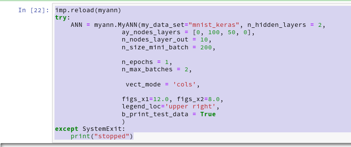
We let the program run in a Jupyter cell with the following parameters:
This produces the following output ( I omitted the output for initialization):
Input data for dataset mnist_keras :
Original shape of X_train = (60000, 28, 28)
Original Shape of y_train = (60000,)
Original shape of X_test = (10000, 28, 28)
Original Shape of y_test = (10000,)

Final input data for dataset mnist_keras :
Shape of X_train = (60000, 784)
Shape of y_train = (60000,)
Shape of X_test = (10000, 784)
Shape of y_test = (10000,)

We have 60000 data sets for training
Feature dimension is 784 (= 28x28)
The number of labels is 10

Shape of y_train = (60000,)
Shape of ay_onehot = (10, 60000)

Values of the enumerate structure for the first 12 elements :
(0, 6)
(1, 8)
(2, 4)
(3, 8)
(4, 6)
(5, 5)
(6, 9)
(7, 1)
(8, 3)
(9, 8)
(10, 9)
(11, 0)

Labels for the first 12 datasets:

Shape of ay_onehot = (10, 60000)
[[0. 0. 0. 0. 0. 0. 0. 0. 0. 0. 0. 1.]
 [0. 0. 0. 0. 0. 0. 0. 1. 0. 0. 0. 0.]
 [0. 0. 0. 0. 0. 0. 0. 0. 0. 0. 0. 0.]
 [0. 0. 0. 0. 0. 0. 0. 0. 1. 0. 0. 0.]
 [0. 0. 1. 0. 0. 0. 0. 0. 0. 0. 0. 0.]
 [0. 0. 0. 0. 0. 1. 0. 0. 0. 0. 0. 0.]
 [1. 0. 0. 0. 1. 0. 0. 0. 0. 0. 0. 0.]
 [0. 0. 0. 0. 0. 0. 0. 0. 0. 0. 0. 0.]
 [0. 1. 0. 1. 0. 0. 0. 0. 0. 1. 0. 0.]
 [0. 0. 0. 0. 0. 0. 1. 0. 0. 0. 1. 0.]]

The node numbers for the 4 layers are :
[784 100  50  10]

Shape of weight matrix between layers 0 and 1 (100, 785)
Creating weight matrix for layer 1 to layer 2
Shape of weight matrix between layers 1 and 2 = (50, 101)
Creating weight matrix for layer 2 to layer 3
Shape of weight matrix between layers 2 and 3 = (10, 51)

The activation function of the standard neurons was defined as "sigmoid"
The activation function gives for z=2.0:  0.8807970779778823

The output function of the neurons in the output layer was defined as "sigmoid"
The output function gives for z=2.0:  0.8807970779778823
num of mini_batches = 300

number of batches : 300
length of first batch : 200
length of last batch : 200

number of epochs = 1
max number of batches = 2

 ---------

Starting epoch 1

 ---------

 Dealing with mini-batch 1

Starting propagation between L0 and L1
Shape of Z_in of layer L0 (without bias) = (784, 200)
Shape of A_out of layer L0 (with bias) = (785, 200)

Starting propagation between L1 and L2
Shape of Z_in of layer L1 (without bias) = (100, 200)
Shape of A_out of layer L1 (with bias) = (101, 200)

Starting propagation between L2 and L3
Shape of Z_in of layer L2 (without bias) = (50, 200)
Shape of A_out of layer L2 (with bias) = (51, 200)

Shape of Z_in of layer L3 = (10, 200)
Shape of A_out of last layer L3 = (10, 200)

 ----

After propagation through all layers:
Shape of Z_in of layer L0 = (784, 200)
Shape of A_out of layer L0 = (785, 200)
Shape of Z_in of layer L1 = (100, 200)
Shape of A_out of layer L1 = (101, 200)
Shape of Z_in of layer L2 = (50, 200)
Shape of A_out of layer L2 = (51, 200)
Shape of Z_in of layer L3 = (10, 200)
Shape of A_out of layer L3 = (10, 200)

 ---------

 Dealing with mini-batch 2

Starting propagation between L0 and L1
Shape of Z_in of layer L0 (without bias) = (784, 200)
Shape of A_out of layer L0 (with bias) = (785, 200)

Starting propagation between L1 and L2
Shape of Z_in of layer L1 (without bias) = (100, 200)
Shape of A_out of layer L1 (with bias) = (101, 200)

Starting propagation between L2 and L3
Shape of Z_in of layer L2 (without bias) = (50, 200)
Shape of A_out of layer L2 (with bias) = (51, 200)

Shape of Z_in of layer L3 = (10, 200)
Shape of A_out of last layer L3 = (10, 200)

 ----

After propagation through all layers:
Shape of Z_in of layer L0 = (784, 200)
Shape of A_out of layer L0 = (785, 200)
Shape of Z_in of layer L1 = (100, 200)
Shape of A_out of layer L1 = (101, 200)
Shape of Z_in of layer L2 = (50, 200)
Shape of A_
out of layer L2 = (51, 200)
Shape of Z_in of layer L3 = (10, 200)
Shape of A_out of layer L3 = (10, 200)


 ------
Total training Time_CPU:  0.010270356000546599

Stopping program regularily
stopped
We see that the dimensions of the Numpy arrays fit our expectations!
If you raise the number for batches and the number for epochs you will pretty soon realize that writing continuous output to a Jupyter cell costs CPU-time. You will also notice strange things regarding performance, multithreading and the use of the Linalg library OpenBlas on Linux system. I have discussed this extensively in a previous article in this blog: Linux, OpenBlas and Numpy matrix multiplications – avoid using all processor cores
So, for another tests we set the following environment variable for the shell in which we start our Jupyter notebook:
export OPENBLAS_NUM_THREADS=4
This is appropriate for my Quad-core CPU with hyperthreading. You may choose a different parameter on your system!
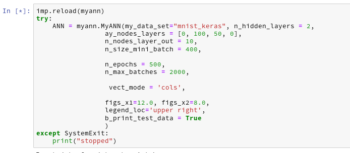
We furthermore stop printing in the epoch loop by editing the call to function “_fit()”:
The node numbers for the 4 layers are :
[784 100  50  10]

Shape of weight matrix between layers 0 and 1 (100, 785)
Creating weight matrix for layer 1 to layer 2
Shape of weight matrix between layers 1 and 2 = (50, 101)
Creating weight matrix for layer 2 to layer 3
Shape of weight matrix between layers 2 and 3 = (10, 51)

The activation function of the standard neurons was defined as "sigmoid"
The activation function gives for z=2.0:  0.8807970779778823

The output function of the neurons in the output layer was defined as "sigmoid"
The output function gives for z=2.0:  0.8807970779778823
num of mini_batches = 150

number of batches : 150
length of first batch : 400
length of last batch : 400


 ------
Total training Time_CPU:  146.44446582399905

Stopping program regularily
stopped
Good !
The time required to repeat this kind of forward propagation for a network with only one hidden layer with 50 neurons and 1000 epochs is around 160 secs. As backward propagation is not much more complex than forward propagation this already indicates that we should be able to train such a most simple MLP with 60000 28×28 images in less than 10 minutes on a standard CPU.
Conclusion
In this article we saw that coding forward propagation is a pretty straight-forward exercise with Numpy! The tricky thing is to understand the way numpy.dot() handles vectorizing of a matrix product and which structure of the matrices is required to get the expected numbers!
Recently, I tested the propagation methods of a small Python3/Numpy class for a multilayer perceptron [MLP]. I unexpectedly ran into a performance problem with OpenBlas.
The problem had to do with the required vectorized matrix operations for forward propagation – in my case through an artificial neural network [ANN] with 4 layers. In a first approach I used 784, 100, 50, 10 neurons in 4 consecutive layers of the MLP. The weight matrices had corresponding dimensions.
The performance problem was caused by extensive multi-threading; it showed a strong dependency on mini-batch sizes and on basic matrix dimensions related to the neuron numbers per layer:
For the given relatively small number of neurons per layer and for mini-batch sizes above a critical value (N > 255) OpenBlas suddenly occupied all processor cores with a 100% work load. This had a disastrous impact on performance.
For neuron numbers as 784, 300, 140, 10 OpenBlas used all processor cores with a 100% work load right from the beginning, i.e. even for small batch sizes. With a seemingly bad performance over all batch sizes – but decreasing somewhat with large batch sizes.
This problem has been discussed elsewhere with respect to the matrix dimensions relevant for the core multiplication and summation operations – i.e. the neuron numbers per layer. However, the vectorizing aspect of matrix multiplications is interesting, too:
One can imagine that splitting the operations for multiple independent test samples is in principle ideal for multi-threading. So, using as many processor cores as possible (in my case 8) does not look like a wrong decision of OpenBlas at first.
Then I noticed that for mini-batch sizes “N” below a certain number (N < 250) the system only seemed to use up to 3-4 cores; so there remained plenty of CPU capacity left for other tasks. Performance for N < 250 was better by at least a factor of 2 compared to a situation with an only slightly bigger batch size (N ≥ 260). I got the impression that OpenBLAS under certain conditions just decides to use as many threads as possible – which no good outcome.
In the last years I sometimes had to work with optimizing multi-threaded database operations on Linux systems. I often got the impression that you have to be careful and leave some CPU resources free for other tasks and to avoid heavy context switching. In addition bottlenecks appeared due to the concurrent access of may processes to the CPU cache. (RAM limitations were an additional factor; but this should not be the case for my Python program.) Furthermore, one should not forget that Python/Numpy experiments on Jupyter notebooks require additional resources to handle the web page output and page update on the browser. And Linux itself also requires some free resources.
So, I wanted to find out whether reducing the number of threads – or available cores – for Numpy and OpenBlas would be helpful in the sense of an overall gain in performance.
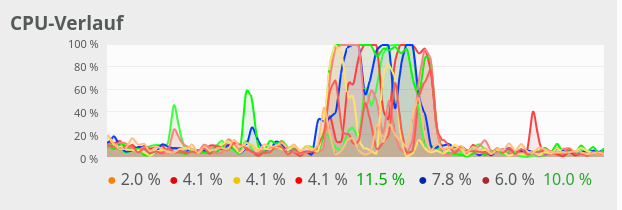
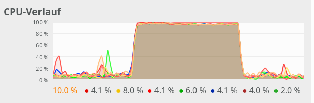
All data shown below were gathered on a desktop system with some background activity due to several open browsers, clementine and pulse-audio as active audio components, an open mail client (kontact), an open LXC container, open Eclipse with Pydev and open ssh connections. Program tests were performed with the help of Jupyter notebooks. Typical background CPU consumption looks like this on Ksysguard:
Most of the consumption is due to audio. Small spikes on one CPU core due to the investigation of incoming mails were possible – but always below 20%.
Basics
One of
the core ingredients to get an ANN running are matrix operations. More precisely: multiplications of 2-dim Numpy matrices (weight matrices) with input vectors. The dimensions of the weight matrices reflect the node-numbers of consecutive ANN-layers. The dimension of the input vector depends on the node number of the lower of two neighbor layers.
However, we perform such matrix operations NOT sequentially sample for sample of a collection of training data – we do it vectorized for so called mini-batches consisting of between 50 and 600000 individual samples of training data. Instead of operating with a matrix on just one feature vector of one training sample we use matrix multiplications whereby the second matrix often comprises many vectors of data samples.
an input layer of 784 nodes (suitable for the MNIST dataset),
one hidden layer with 100 nodes,
another hidden layer with 50 nodes
and an output layer of 10 nodes (fitting again the MNIST dataset)
and “mini”-batches of different sizes (between 20 and 20000). An input vector to the first hidden layer has a dimension of 100, so the weight matrix creating this input vector from the “output” of the MLP’s input layer has a shape of 784×100. Multiplication and summation in this case is done over the dimension covering 784 features. When we work with mini-batches we want to do these operations in parallel for as many elements of a mini-batch as possible.
All in all we have to perform 3 matrix operations
(784×100) matrix on (784)-vector, (100×50) matrix on (100)-vector, (50×10) matrix on (50) vector
on our example ANN with 4 layers. However, we collect the data for N mini-batch samples in an array. This leads to Numpy matrix multiplications of the kind
(784×100) matrix on an (784, N)-array, (100×50) matrix on an (100, N)-array, (50×10) matrix on an (50, N)-array.
Thus, we deal with matrix multiplications of two 2-dim matrices. Linear algebra libraries should optimize such operations for different kinds of processors.
The reaction of OpenBlas to an MLP with 4 layers comprising 784, 100, 50, 10 nodes
On my Linux system Python/Numpy use the openblas-library. This is confirmed by the output of command “np.__config__.show()”:
openblas_info:
    libraries = ['openblas', 'openblas']
    library_dirs = ['/usr/local/lib']
    language = c
    define_macros = [('HAVE_CBLAS', None)]
blas_opt_info:
    libraries = ['openblas', 'openblas']
    library_dirs = ['/usr/local/lib']
    language = c
    define_macros = [('HAVE_CBLAS', None)]
openblas_lapack_info:
    libraries = ['openblas', 'openblas']
    library_dirs = ['/usr/local/lib']
    language = c
    define_macros = [('HAVE_CBLAS', None)]
lapack_opt_info:
    libraries = ['openblas', 'openblas']
    library_dirs = ['/usr/local/lib']
    language = c
    define_macros = [('HAVE_CBLAS', None)]
and repeated the full forward propagation 30 times (corresponding to 30 epochs in a full training series – but here without cost calculation and weight adjustment. I just did forward propagation.)
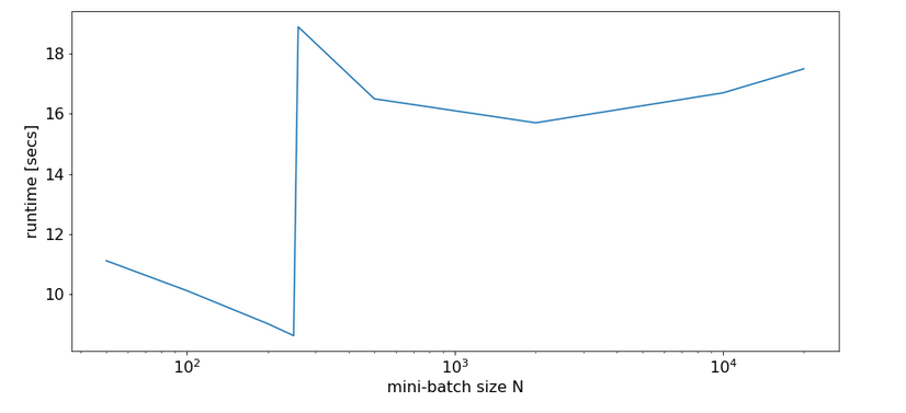
In a first experiment, I did not artificially limit the number of cores to be used. Measured response times in seconds are indicated in the following plot:
Runtime for a free number of cores to use and different batch-sizes N
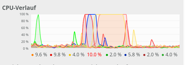
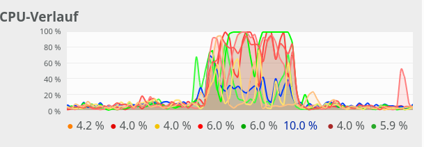
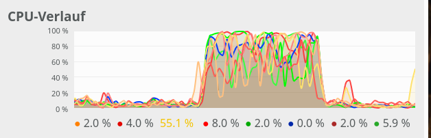
We see that something dramatic happens between a batch size of 250 and 260. Below you see the plots for CPU core consumption for N=50, N=200, N=250, N=260 and N=2000.
N=50:
N=200:
N=250:
N=260:
N=2000:
The plots indicate that everything goes well up to N=250. Up to this point around 4 cores are used – leaving 4 cores relatively free. After N=260 OpenBlas decides to use all 8 cores with a load of 100% – and performance suffers by more than a factor of 2.
This result support the idea to look for an optimum of the number of cores “C” to use.
The reaction of OpenBlas to an MLP with layers comprising 784, 300, 140, 10 nodes
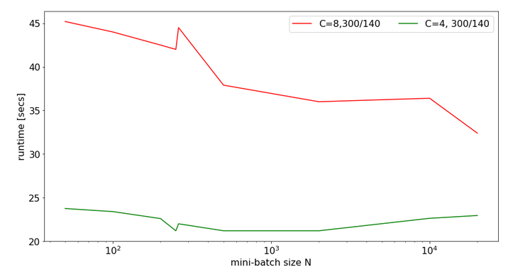
For a MLP with neuron numbers (784, 300, 140, 10) I got the red curve for response time in the plot below. The second curve shows what performance is possible with just using 4 cores:
Note the significantly higher response times. We also see again that something strange happens at the change of the batch-size from 250 to 260.
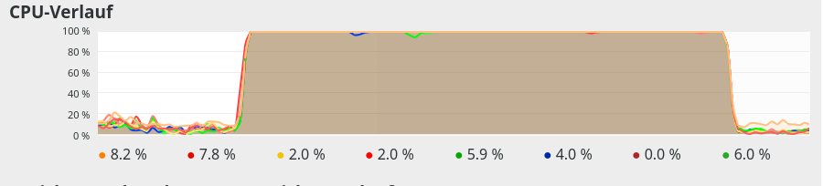
The 100% CPU
consumption even for a batch-size of only 50 is shown below:
Though different from the first test case also these plots indicate that – somewhat paradoxically – reducing the number of CPU cores available to OpenBlas could have a performance enhancing effect.
Limiting the number of available cores to OpenBlas
A bit of Internet research shows that one can limit the number of cores to use by OpenBlas e.g. via an environment variable for the shell, in which we start a Jupyter notebook. The relevant command to limit the number of cores “C” to 3 is :
export OPENBLAS_NUM_THREADS=3
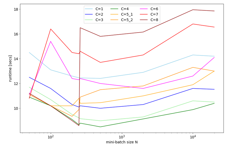
Below you find plots for the response times required for the batch sizes N listed above and core numbers of
C=1, C=2, C=3, C=4, C=5, C=6, C=7, C=8 :
For C=5 I did 2 different runs; the different results for C=5 show that the system reacts rather sensitively. It changes its behavior for larger core number drastically.
We also find an overall minimum of the response time: The overall optimum occurs for 400 < N < 500 for C=1, 2, 3, 4 – with the minimum region being broadest for C=3. The absolute minimum is reached on my CPU for C=4.
We understand from the plots above that the number of cores to use become hyper-parameters for the tuning of the performance of ANNs – at least as long as a standard multicore-CPU is used.
CPU-consumption
CPU consumption for N=50 and C=2 looks like:
For comparison see the CPU consumption for N=20000 and C=4:
CPU consumption for N=20000 and C=6:
We see that between C=5 and C=6 CPU resources get heavily consumed; there are almost no reserves left in the Linux system for C ≥ 6.
Dependency on the size of the weight-matrices and the node numbers
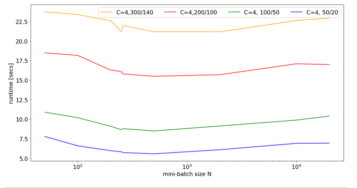
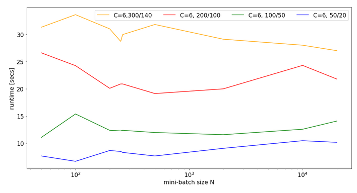
For a full view on the situation I also looked at the response time variation with node numbers for a given number of CPU cores.
For C=4 and node number cases
784, 300, 140, 10
784, 200, 100, 10
784, 100, 50, 10
784, 50, 20, 10
I got the following results:
There is some broad variation with the weight-matrix size; the bigger the weight-matrix the longer the calculation time. This is, of course, to be expected. Note that the variation with the batch-size number is relatively smooth – with an optimum around 400.
Now, look at the same plot for C=6:
Note that the response time is significantly bigger in all cases compared to the previous situation with C=4. In cases of a large matrix by around 36% for N=2000. Also the variation with batch-size is more pronounced.
Still, even with 6 cores you do not get factors between 1.4 and 2.0 as compared to the case of C=8 (see above)!
Conclusion
As I do not know what the authors of OpenBlas are doing exactly, I refrain from technically understanding and interpreting the causes of the data shown above.
However, some consequences seem to be clear:
It is a bad idea to provide all CPU cores to OpenBlas – which unfortunately is the default.
The data above indicate that using only 4 out of 8 core threads is reasonable to get an optimum performance for vectorized matrix multiplications on my CPU.
Not leaving at least 2 CPU cores free for other tasks is punished by significant performance losses.
When leaving the decision of how many cores to use to OpenBlas a critical batch-size may exist for which the performance suddenly breaks down due to heavy multi-threading.
Whenever you deal with ANN or MLP simulations on a standard CPU (not GPU!) you should absolutely care about how many cores and related threads you want to offer to OpenBlas. As far as I understood from some Internet articles the number of cores to be used can be not only be controlled by Linux (shell) environment variables but also by os-commands in a Python program. You should perform tests to find optimum values for your CPU.