MLP, Numpy, TF2 – performance issues – Step III – a correction to BW propagation

In the last articles of this series

MLP, Numpy, TF2 – performance issues – Step II – bias neurons, F- or C- contiguous arrays and performance
MLP, Numpy, TF2 – performance issues – Step I – float32, reduction of back propagation

we looked at the FW-propagation of the MLP code which I discussed in another article series. We found that the treatment of bias neurons in the input layer was technically inefficient due to a collision of C- and F-contiguous arrays. By circumventing the problem we could accelerate the FW-propagation of big batches (as the complete training or test data set) by more than a factor of 2.

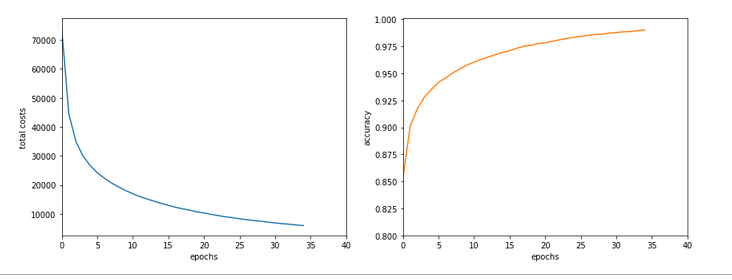
In this article I want to turn to the BW propagation and do some analysis regarding CPU consumption there. We will find a simple (and stupid) calculation step there which we shall replace. This will give us another 15% to 22% performance improvement in comparison to what we have reached in the last article for MNIST data:

  • 9.6 secs for 35 epochs and a batch-size of 500
  • and 8.7 secs for a batch-size of 20000.

Present CPU time relation between the FW- and the BW-propagation

The central training of mini-batches is performed by the method “_handle_mini_batch()”.

#
    ''' -- Method to deal with a batch -- '''
    def _handle_mini_batch (self, num_batch = 0, num_epoch = 0, b_print_y_vals = False, b_print = False, b_keep_bw_matrices = True):
        ''' .... '''
        # Layer-related lists to be filled with 2-dim Numpy matrices during FW propagation
        # ********************************************************************************
        li_Z_in_layer  = [None] * self._n_total_layers # List of matrices with z-input values for each layer; filled during FW-propagation
        li_A_out_layer = li_Z_in_layer.copy()          # List of matrices with results of activation/output-functions for each layer; filled during FW-propagation
        li_delta_out   = li_Z_in_layer.copy()          # Matrix with out_delta-values at the outermost layer 
        li_delta_layer = li_Z_in_layer.copy()          # List of the matrices for the BW propagated delta values 
        li_D_layer     = li_Z_in_layer.copy()          # List of the derivative matrices D containing partial derivatives of the activation/ouput functions 
        li_grad_layer  = li_Z_in_layer.copy()          # List of the matrices with gradient values for weight corrections
        
        # Major steps for the mini-batch during one epoch iteration 
        # **********************************************************
        
        #ts=time.perf_counter()
        # Step 0: List of indices for data records in the present mini-batch
        # ******
        ay_idx_batch = self._ay_mini_batches[num_batch]
        
        # Step 1: Special preparation of the Z-input to the MLP's input Layer L0
        # ******
        # ts=time.perf_counter()
        # slicing 
        li_Z_in_layer[0] = self._X_train[ay_idx_batch] # numpy arrays can be indexed by an array of integers
        
        # transposition 
        #~~~~~~~~~~~~~~
        li_Z_in_layer[0] = li_Z_in_layer[0].T
        #te=time.perf_counter(); t_batch = te - ts;
        #print("\nti - transposed inputbatch =", t_batch)
        
        # Step 2: Call forward propagation method for the present mini-batch of training records
        # *******
n        #tsa = time.perf_counter() 
        self._fw_propagation(li_Z_in = li_Z_in_layer, li_A_out = li_A_out_layer) 
        #tea = time.perf_counter(); ta = tea - tsa;  print("ta - FW-propagation", "%10.8f"%ta)
        
        # Step 3: Cost calculation for the mini-batch 
        # ********
        #tsb = time.perf_counter() 
        ay_y_enc = self._ay_onehot[:, ay_idx_batch]
        ay_ANN_out = li_A_out_layer[self._n_total_layers-1]
        total_costs_batch, rel_reg_contrib = self._calculate_loss_for_batch(ay_y_enc, ay_ANN_out, b_print = False)
        # we add the present cost value to the numpy array 
        self._ay_costs[num_epoch, num_batch]            = total_costs_batch
        self._ay_reg_cost_contrib[num_epoch, num_batch] = rel_reg_contrib
        #teb = time.perf_counter(); tb = teb - tsb; print("tb - cost calculation", "%10.8f"%tb)
        
        
        # Step 4: Avg-error for later plotting 
        # ********
        #tsc = time.perf_counter() 
        # mean "error" values - averaged over all nodes at outermost layer and all data sets of a mini-batch 
        ay_theta_out = ay_y_enc - ay_ANN_out
        ay_theta_avg = np.average(np.abs(ay_theta_out)) 
        self._ay_theta[num_epoch, num_batch] = ay_theta_avg 
        #tec = time.perf_counter(); tc = tec - tsc; print("tc - error", "%10.8f"%tc)
        
        
        # Step 5: Perform gradient calculation via back propagation of errors
        # ******* 
        #tsd = time.perf_counter() 
        self._bw_propagation( ay_y_enc = ay_y_enc, 
                              li_Z_in = li_Z_in_layer, 
                              li_A_out = li_A_out_layer, 
                              li_delta_out = li_delta_out, 
                              li_delta = li_delta_layer,
                              li_D = li_D_layer, 
                              li_grad = li_grad_layer, 
                              b_print = b_print,
                              b_internal_timing = False 
                              ) 
        #ted = time.perf_counter(); td = ted - tsd; print("td - BW propagation", "%10.8f"%td)
        
        # Step 7: Adjustment of weights  
        # *******        
        #tsf = time.perf_counter() 
        rg_layer=range(0, self._n_total_layers -1)
        for N in rg_layer:
            delta_w_N = self._learn_rate * li_grad_layer[N]
            self._li_w[N] -= ( delta_w_N + (self._mom_rate * self._li_mom[N]) )
            
            # save momentum
            self._li_mom[N] = delta_w_N
        #tef = time.perf_counter(); tf = tef - tsf; print("tf - weight correction", "%10.8f"%tf)
        
        return None


I took some time measurements there:

ti - transposed inputbatch = 0.0001785
ta - FW-propagation 0.00080975
tb - cost calculation 0.00030705
tc - error 0.00016182
td - BW propagation 0.00112558
tf - weight correction 0.00020079

ti - transposed inputbatch = 0.00018144
ta - FW-propagation 0.00082022
tb - cost calculation 0.00031284
tc - error 0.00016652
td - BW propagation 0.00106464
tf - weight correction 0.00019576

You see that the FW-propagation is a bit faster than the BW-propagation. This is a bit strange as the FW-propagation is dominated meanwhile by a really expensive operation which we cannot accelerate (without choosing a new activation function): The calculation of the sigmoid value for the inputs at layer L1.

So let us look into the BW-propagation; the code for it is momentarily:

    ''' -- Method to handle error BW propagation for a mini-batch --'''
    def _bw_propagation(self, 
                        ay_y_enc, li_Z_in, li_A_out, 
                        li_delta_out, li_delta, li_D, li_
grad, 
                        b_print = True, b_internal_timing = False):
        
        # List initialization: All parameter lists or arrays are filled or to be filled by layer operations 
        # Note: the lists li_Z_in, li_A_out were already filled by _fw_propagation() for the present batch 
        
        # Initiate BW propagation - provide delta-matrices for outermost layer
        # *********************** 
        tsa = time.perf_counter() 
        # Input Z at outermost layer E  (4 layers -> layer 3)
        ay_Z_E = li_Z_in[self._n_total_layers-1]
        # Output A at outermost layer E (was calculated by output function)
        ay_A_E = li_A_out[self._n_total_layers-1]
        
        # Calculate D-matrix (derivative of output function) at outmost the layer - presently only D_sigmoid 
        ay_D_E = self._calculate_D_E(ay_Z_E=ay_Z_E, b_print=b_print )
        #ay_D_E = ay_A_E * (1.0 - ay_A_E)

        # Get the 2 delta matrices for the outermost layer (only layer E has 2 delta-matrices)
        ay_delta_E, ay_delta_out_E = self._calculate_delta_E(ay_y_enc=ay_y_enc, ay_A_E=ay_A_E, ay_D_E=ay_D_E, b_print=b_print) 
        
        # add the matrices to their lists ; li_delta_out gets only one element 
        idxE = self._n_total_layers - 1
        li_delta_out[idxE] = ay_delta_out_E # this happens only once
        li_delta[idxE]     = ay_delta_E
        li_D[idxE]         = ay_D_E
        li_grad[idxE]      = None    # On the outermost layer there is no gradient ! 
        
        tea = time.perf_counter(); ta = tea - tsa; print("\nta-bp", "%10.8f"%ta)
        
        # Loop over all layers in reverse direction 
        # ******************************************
        # index range of target layers N in BW direction (starting with E-1 => 4 layers -> layer 2))
        range_N_bw_layer = reversed(range(0, self._n_total_layers-1))   # must be -1 as the last element is not taken 
        
        # loop over layers 
        tsb = time.perf_counter() 
        for N in range_N_bw_layer:
            
            # Back Propagation operations between layers N+1 and N 
            # *******************************************************
            # this method handles the special treatment of bias nodes in Z_in, too
            tsib = time.perf_counter() 
            ay_delta_N, ay_D_N, ay_grad_N = self._bw_prop_Np1_to_N( N=N, li_Z_in=li_Z_in, li_A_out=li_A_out, li_delta=li_delta, b_print=False )
            teib = time.perf_counter(); tib = teib - tsib; print("N = ", N, " tib-bp", "%10.8f"%tib)
            
            # add matrices to their lists 
            #tsic = time.perf_counter() 
            li_delta[N] = ay_delta_N
            li_D[N]     = ay_D_N
            li_grad[N]= ay_grad_N
            #teic = time.perf_counter(); tic = teic - tsic; print("\nN = ", N, " tic = ", "%10.8f"%tic)
        teb = time.perf_counter(); tb = teb - tsb; print("tb-bp", "%10.8f"%tb)
       
        return


Typical timing results are:

ta-bp 0.00007112
N =  2  tib-bp 0.00025399
N =  1  tib-bp 0.00051683
N =  0  tib-bp 0.00035941
tb-bp 0.00126436

ta-bp 0.00007492
N =  2  tib-bp 0.00027644
N =  1  tib-bp 0.00090043
N =  0  tib-bp 0.00036728
tb-bp 0.00168378

We see that the CPU consumption of “_bw_prop_Np1_to_N()” should be analyzed in detail. It is relatively time consuming at every layer, but especially at layer L1. (The list adds are insignificant.)
What does this method presently look like?

    ''' -- Method to calculate the BW-propagated delta-matrix and the gradient matrix to/for layer N '''
    def _bw_prop_Np1_to_N(self, N, li_Z_in, li_A_out, li_delta, b_print=False):
        '''
        BW-
error-propagation between layer N+1 and N 
        Version 1.5 - partially accelerated 

        Inputs: 
            li_Z_in:  List of input Z-matrices on all layers - values were calculated during FW-propagation
            li_A_out: List of output A-matrices - values were calculated during FW-propagation
            li_delta: List of delta-matrices - values for outermost ölayer E to layer N+1 should exist 
        
        Returns: 
            ay_delta_N - delta-matrix of layer N (required in subsequent steps)
            ay_D_N     - derivative matrix for the activation function on layer N 
            ay_grad_N  - matrix with gradient elements of the cost fnction with respect to the weights on layer N 
        '''
        
        # Prepare required quantities - and add bias neuron to ay_Z_in 
        # ****************************
        
        # Weight matrix meddling between layers N and N+1 
        ay_W_N = self._li_w[N]

        # delta-matrix of layer N+1
        ay_delta_Np1 = li_delta[N+1]

        # fetch output value saved during FW propagation 
        ay_A_N = li_A_out[N]

        # Optimization V1.5 ! 
        if N > 0: 
            
            #ts=time.perf_counter()
            ay_Z_N = li_Z_in[N]
            # !!! Add intermediate row (for bias) to Z_N !!!
            ay_Z_N = self._add_bias_neuron_to_layer(ay_Z_N, 'row')
            #te=time.perf_counter(); t1 = te - ts; print("\nBW t1 = ", t1, " N = ", N) 
        
            # Derivative matrix for the activation function (with extra bias node row)
            # ********************
            #    can only be calculated now as we need the z-values
            #ts=time.perf_counter()
            ay_D_N = self._calculate_D_N(ay_Z_N)
            #te=time.perf_counter(); t2 = te - ts; print("\nBW t2 = ", t2, " N = ", N) 
            
            # Propagate delta
            # **************

            # intermediate delta 
            # ~~~~~~~~~~~~~~~~~~
            #ts=time.perf_counter()
            ay_delta_w_N = ay_W_N.T.dot(ay_delta_Np1)
            #te=time.perf_counter(); t3 = te - ts; print("\nBW t3 = ", t3) 
            
            # final delta 
            # ~~~~~~~~~~~
            #ts=time.perf_counter()
            ay_delta_N = ay_delta_w_N * ay_D_N
            
            # Orig reduce dimension again
            # **************************** 
            ay_delta_N = ay_delta_N[1:, :]
            #te=time.perf_counter(); t4 = te - ts; print("\nBW t4 = ", t4) 
            
        else: 
            ay_delta_N = None
            ay_D_N = None
        
        # Calculate gradient
        # ********************
        #ts=time.perf_counter()
        ay_grad_N = np.dot(ay_delta_Np1, ay_A_N.T)
        #te=time.perf_counter(); t5 = te - ts; print("\nBW t5 = ", t5) 
        
        # regularize gradient (!!!! without adding bias nodes in the L1, L2 sums) 
        #ts=time.perf_counter()
        if self._lambda2_reg > 0: 
            ay_grad_N[:, 1:] += self._li_w[N][:, 1:] * self._lambda2_reg 
        if self._lambda1_reg > 0: 
            ay_grad_N[:, 1:] += np.sign(self._li_w[N][:, 1:]) * self._lambda1_reg 
        #te=time.perf_counter(); t6 = te - ts; print("\nBW t6 = ", t6) 
        
        return ay_delta_N, ay_D_N, ay_grad_N

 
Timing data for a batch-size of 500 are:

N =  2
BW t1 =  0.0001169009999557602  N =  2
BW t2 =  0.00035331499998392246  N =  2
BW t3 =  0.00018078099992635543
BW t4 =  0.00010234199999104021
BW t5 =  9.928200006470433e-05
BW t6 =  2.4267000071631628e-05
N =  2  tib-bp 0.00124414

N =  1
BW t1 =  0.0004323499999827618  N =  1
BW t2 =  0.
000781415999881574  N =  1
BW t3 =  4.2077999978573644e-05
BW t4 =  0.00022921000004316738
BW t5 =  9.376399998473062e-05
BW t6 =  0.00012183700005152787
N =  1  tib-bp 0.00216281

N =  0
BW t5 =  0.0004289769999559212
BW t6 =  0.00015404999999191205
N =  0  tib-bp 0.00075249
....
N =  2
BW t1 =  0.00012802800006284087  N =  2
BW t2 =  0.00034988200013685855  N =  2
BW t3 =  0.0001854429999639251
BW t4 =  0.00010359299994888715
BW t5 =  0.00010210400000687514
BW t6 =  2.4010999823076418e-05
N =  2  tib-bp 0.00125854

N =  1
BW t1 =  0.0004407169999467442  N =  1
BW t2 =  0.0007845899999665562  N =  1
BW t3 =  0.00025684100000944454
BW t4 =  0.00012409999999363208
BW t5 =  0.00010345399982725212
BW t6 =  0.00012994100006835652
N =  1  tib-bp 0.00221321

N =  0
BW t5 =  0.00044504700008474174
BW t6 =  0.00016473000005134963
N =  0  tib-bp 0.00071442

....
N =  2
BW t1 =  0.000292730999944979  N =  2
BW t2 =  0.001102525000078458  N =  2
BW t3 =  2.9429999813146424e-05
BW t4 =  8.547999868824263e-06
BW t5 =  3.554099998837046e-05
BW t6 =  2.5041999833774753e-05
N =  2  tib-bp 0.00178565

N =  1
BW t1 =  3.143399999316898e-05  N =  1
BW t2 =  0.0006720640001276479  N =  1
BW t3 =  5.4785999964224175e-05
BW t4 =  9.756200006449944e-05
BW t5 =  0.0001605449999715347
BW t6 =  1.8391000139672542e-05
N =  1  tib-bp 0.00147566

N =  0
BW t5 =  0.0003641810001226986
BW t6 =  6.338999992294703e-05
N =  0  tib-bp 0.00046542

 
It seems that we should care about t1, t2, t3 for hidden layers and maybe about t5 at layers L1/L0.

However, for a batch-size of 15000 things look a bit different:

N =  2
BW t1 =  0.0005776280000304723  N =  2
BW t2 =  0.004995969999981753  N =  2
BW t3 =  0.0003165199999557444
BW t4 =  0.0005244750000201748
BW t5 =  0.000518499999998312
BW t6 =  2.2458999978880456e-05
N =  2  tib-bp 0.00736144

N =  1
BW t1 =  0.0010120430000029046  N =  1
BW t2 =  0.010797029000002567  N =  1
BW t3 =  0.0005006920000028003
BW t4 =  0.0008704929999794331
BW t5 =  0.0010805200000163495
BW t6 =  3.0326000000968634e-05
N =  1  tib-bp 0.01463436

N =  0
BW t5 =  0.006987539000022025
BW t6 =  0.00023552499999368592
N =  0  tib-bp 0.00730959


N =  2
BW t1 =  0.0006299790000525718  N =  2
BW t2 =  0.005081416999985322  N =  2
BW t3 =  0.00018547400003399162
BW t4 =  0.0005970070000103078
BW t5 =  0.000564008000026206
BW t6 =  2.3311000006742688e-05
N =  2  tib-bp 0.00737899

N =  1
BW t1 =  0.0009376909999900818  N =  1
BW t2 =  0.010650266999959968  N =  1
BW t3 =  0.0005232729999988806
BW t4 =  0.0009100700000317374
BW t5 =  0.0011237720000281115
BW t6 =  0.00016643800000792908
N =  1  tib-bp 0.01466144

N =  0
BW t5 =  0.006987463000029948
BW t6 =  0.00023978600000873485
N =  0  tib-bp 0.00734308

 
For big batch-sizes “t2” dominates everything. It seems that we have found another code area which causes the trouble with big batch-sizes which we already observed before!

What operations do the different CPU times stand for?

To keep an overview without looking into the code again, I briefly summarize which operations cause which of the measured time differences:

  • t1” – which contributes for small batch-sizes stands for adding a bias neuron to the input data Z_in at each layer.
  • t2” – which is by far dominant for big batch sizes stands for calculating the derivative of the output/activation function (in our case of the sigmoid function) at the various layers.
  • t3” – which contributes at
    some layers stands for a dot()-matrix multiplication with the transposed weight-matrix,
  • t4” – covers an element-wise matrix-multiplication,
  • t5” – contributes at the BW-transition from layer L1 to L0 and covers the matrix multiplication there (including the full output matrix with the bias neurons at L0)

Use the output values calculated at each layer during FW-propagation!

Why does the calculation of the derivative of the sigmoid function take so much time? Answer: Because I coded it stupidly! Just look at it:

    ''' -- Method to calculate the matrix with the derivative values of the output function at outermost layer '''
    def _calculate_D_N(self, ay_Z_N, b_print= False):
        '''
        This method calculates and returns the D-matrix for the outermost layer
        The D matrix contains derivatives of the output function with respect to local input "z_j" at outermost nodes. 
        
        Returns
        ------
        ay_D_E:    Matrix with derivative values of the output function 
                   with respect to local z_j valus at the nodes of the outermost layer E
        Note: This is a 2-dim matrix over layer nodes and training samples of the mini-batch
        '''
        if self._my_out_func == 'sigmoid':
            ay_D_E = self._D_sigmoid(ay_Z = ay_Z_N)
        
        else:
            print("The derivative for output function " + self._my_out_func + " is not known yet!" )
            sys.exit()
        
        return ay_D_E

    ''' -- method for the derivative of the sigmoid function-- '''
    def _D_sigmoid(self, ay_Z):
        ''' 
        Derivative of sigmoid function with respect to Z-values 
        - works via expit element-wise on matrices
        Input:  Z - Matrix with Input values for the activation function Phi() = sigmoid() 
        Output: D - Matrix with derivative values 
        '''
        S_Z = self._sigmoid(ay_Z)
        return S_Z * (1.0 - S_Z)

 
We first call an intermediate function which then directs us to the right function for a chosen activation function. Well meant: So far, we use only the sigmoid function, but it could e.g. also be the relu() or tanh()-function. So, we did what we did for the sake of generalization. But we did it badly because of two reasons:

  • We did not keep up a function call pattern which we introduced in the FW-propagation.
  • The calculation of the derivative is inefficient.

The first point is a minor one: During FW-propagation we called the right (!) activation function, i.e. the one we choose by input parameters to our ANN-object, by an indirect call. Why not do it the same way here? We would avoid an intermediate function call and keep up a pattern. Actually, we prepared the necessary definitions already in the __init__()-function.

The second point is relevant for performance: The derivative function produces the correct results for a given “ay_Z”, but this is totally inefficient in our BW-situation. The code repeats a really expensive operation which we have already performed during FW-propagation: calling sigmoid(ay_Z) to get “A_out”-values per layer then. We even put the A_out-values [=sigmoid(ay_Z_in)] per layer and batch (!) with some foresight into a list in “li_A_out[]” at that point of the code (see the FW-propagation code discussed in the last article).

So, of course, we should use these “A_out”-values now in the BW-steps! No further comment …. you see what we need to do.

Hint: Actually, also other activation functions “act(Z)” like e.g. the “tanh()”-function have derivatives which depend on on “A=act(
Z)”, only. So, we should provide Z and A via an interface to the derivative function and let the respective functions take what it needs.
But, my insight into my own dumbness gets worse.

Eliminate the bias neuron operation!

Why did we need a bias-neuron operation? Answer: We do not need it! It was only introduced due to insufficient cleverness. In the article

A simple Python program for an ANN to cover the MNIST dataset – VII – EBP related topics and obstacles

I have already indicated that we use the function for adding a row of bias-neurons again only to compensate one deficit: The matrix of the derivative values did not fit the shape of the weight matrix for the required element-wise operations. However, I also said: There probably is an alternative.

Well, let me make a long story short: The steps behind t1 up to t4 to calculate “ay_delta_N” for the present layer L_N (with N>=1) can be compressed into two relatively simple lines:

ay_delta_w_N = ay_W_N.T.dot(ay_delta_Np1)
ay_delta_N = ay_delta_w_N[1:,:] * ay_A_N[1:,:] * (1.0 – ay_A_N[1:,:]); ay_D_N = None;

No bias back and forth corrections! Instead we use simple slicing to compensate for our weight matrices with a shape covering an extra row of bias node output. No Z-based derivative calculation; no sigmoid(Z)-call. The last statement is only required to support the present output interface. Think it through in detail; the shortcut does not cause any harm.

Code change for tests

Before we bring the code into a new consolidated form with re-coded methods let us see what we gain by just changing the code to the two lines given above in terms of CPU time and performance. Our function “_bw_prop_Np1_to_N()” then gets reduced to the following lines:

    ''' -- Method to calculate the BW-propagated delta-matrix and the gradient matrix to/for layer N '''
    def _bw_prop_Np1_to_N(self, N, li_Z_in, li_A_out, li_delta, b_print=False):
        
        # Weight matrix meddling between layers N and N+1 
        ay_W_N = self._li_w[N]
        ay_delta_Np1 = li_delta[N+1]

        # fetch output value saved during FW propagation 
        ay_A_N = li_A_out[N]

        # Optimization from previous version  
        if N > 0: 
            #ts=time.perf_counter()
            ay_Z_N = li_Z_in[N]
            
            # Propagate delta
            # ~~~~~~~~~~~~~~~~~
            ay_delta_w_N = ay_W_N.T.dot(ay_delta_Np1)
            ay_delta_N = ay_delta_w_N[1:,:] * ay_A_N[1:,:] * (1.0 - ay_A_N[1:,:])
            ay_D_N = None; 
            
        else: 
            ay_delta_N = None
            ay_D_N = None
        
        # Calculate gradient
        # ********************
        ay_grad_N = np.dot(ay_delta_Np1, ay_A_N.T)
        
        if self._lambda2_reg > 0: 
            ay_grad_N[:, 1:] += self._li_w[N][:, 1:] * self._lambda2_reg 
        if self._lambda1_reg > 0: 
            ay_grad_N[:, 1:] += np.sign(self._li_w[N][:, 1:]) * self._lambda1_reg 
        
        return ay_delta_N, ay_D_N, ay_grad_N


Performance gain

What run times do we get with this setting? We perform our typical test runs over 35 epochs – but this time for two different batch-sizes:

Batch-size = 500

 
------------------
Starting epoch 35

Time_CPU for epoch 35 0.2169024469985743
Total CPU-time:  7.52385053600301

learning rate =  0.0009994051838157095

total costs of training set   =  -1.0
rel. reg. contrib. to total costs =  -1.0

total costs 
of last mini_batch   =  65.43618
rel. reg. contrib. to batch costs =  0.12302863

mean abs weight at L0 :  -10.0
mean abs weight at L1 :  -10.0
mean abs weight at L2 :  -10.0

avg total error of last mini_batch =  0.00758
presently batch averaged accuracy   =  0.99272

-------------------
Total training Time_CPU:  7.5257336139984545

Not bad! We became faster by around 2 secs compared to the results of the last article! This is close to an improvement of 20%.

But what about big batch sizes? Here is the result for a relatively big batch size:

Batch-size = 20000

------------------
Starting epoch 35

Time_CPU for epoch 35 0.2019189490019926
Total CPU-time:  6.716679593999288

learning rate =  9.994051838157101e-05

total costs of training set   =  -1.0
rel. reg. contrib. to total costs =  -1.0

total costs of last mini_batch   =  13028.141
rel. reg. contrib. to batch costs =  0.00021923862

mean abs weight at L0 :  -10.0
mean abs weight at L1 :  -10.0
mean abs weight at L2 :  -10.0

avg total error of last mini_batch =  0.04389
presently batch averaged accuracy   =  0.95602

-------------------
Total training Time_CPU:  6.716954112998792

Again an acceleration by roughly 2 secs – corresponding to an improvement of 22%!

In both cases I took the best result out of three runs.

Conclusion

Enough for today! We have done a major step with regard to performance optimization also in the BW-propagation. It remains to re-code the derivative calculation in form which uses indirect function calls to remain flexible. I shall give you the code in the next article.

We learned today is that we, of course, should reuse the results of the FW-propagation and that it is indeed a good investment to save the output data per layer in some Python list or other suitable structures during FW-propagation. We also saw again that a sufficiently efficient bias neuron treatment can be achieved by a more efficient solution than provisioned so far.

All in all we have meanwhile gained more than a factor of 6.5 in performance since we started with optimization. Our new standard values are 7.3 secs and 6.8 secs for 35 epochs on MNIST data and batch sizes of 500 and 20000, respectively.

We have reached the order of what Keras and TF2 can deliver on a CPU for big batch sizes. For small batch sizes we are already faster. This indicates that we have done no bad job so far …

In the next article we shall look a bit at the matrix operations and evaluate further optimization options.

MLP, Numpy, TF2 – performance issues – Step II – bias neurons, F- or C- contiguous arrays and performance

Welcome back, my friends of MLP coding. In the last article we gave the code developed in the article series

A simple Python program for an ANN to cover the MNIST dataset – I – a starting point

a first performance boost by two simple measures:

  • We set all major arrays to the “numpy.float32” data type instead of the default “float64”.
  • In addition we eliminated superfluous parts of the backward [BW] propagation between the first hidden layer and the input layer.

This brought us already down to around

11 secs for 35 epochs on the MNIST dataset, a batch-size of 500 and an accuracy around 99 % on the training set

This was close to what Keras (and TF2) delivered for the same batch size. It marks the baseline for further performance improvements of our MLP code.

Can we get better than 11 secs for 35 epochs? The answer is: Yes, we can – but only in small steps. So, do not expect any gigantic performance leaps for the training loop itself. But, there was and is also our observation that there is no significant acceleration with growing batch sizes over 1000 – but with Keras we saw such an acceleration.

In this article I shall shortly discuss why we should care about big batch sizes – at least in combination with FW-propagation. Afterwards I want to draw your attention to a specific code segment of our MLP. We shall see that an astonishingly simple array operation dominates the CPU time of our straight forward coded FW propagation. Especially for big batch sizes!

Actually, it is an operation I would never have guessed to be such an an obstacle to efficiency if somebody had asked me. As a naive Python beginner I had to learn that the arrangement of arrays in the computer’s memory sometimes have an impact – especially when big arrays are involved. To get to this generally useful insight we will have to invest some effort into performance tests of some specific Numpy operations on arrays. The results give us some options for possible performance improvements; but in the end we shall circumvent the impediment all together.

The discussion will indicate that we should change our treatment of bias neurons fundamentally. We shall only go a preliminary step in this direction. This step will give us already a 15% improvement regarding the training time. But even more important, it will reward us with a significant improvement – by a factor > 2.5 – with respect to the FW-propagation of the complete training and test data sets, i.e. for the FW-propagation of “batches” with big sizes (60000 or 10000 samples).

“np.” abbreviates the “Numpy” library below. I shall sometimes speak of our 2-dimensional Numpy “arrays” as “matrices” in an almost synonymous way. See, however, one of the links at the bottom of the article for the subtle differences of related data types. For the time being we can safely ignore the mathematical differences between matrices, stacks of matrices and tensors. But we should have a clear understanding of the profound difference between the “*“-operation and the “np.dot()“-operation on 2-dimensional arrays.

Why are big batch sizes relevant?

There are several reasons why we should care about an efficient treatment of big batches. I name a few, only:

  • Numpy operations on bigger matrices may become more efficient on systems with multiple CPUs, CPU cores or multiple GPUs.
  • Big batch sizes together with a relatively small learning rate will lead to a smoother descent path on the cost hyperplane. Could become important in some intricate real life scenarios beyond MNIST.
  • We should test the achieved accuracy on evaluation and test datasets during training. This data sets may have a much bigger size than the training batches.

The last point addresses the problem of overfitting: We may approach a minimum of the loss function of the training data set, but may leave the minimum of the cost function (and of related errors) of the test data set at some point. Therefore, we should check the accuracy on evaluation and test data sets already during the training phase. This requires the FW-propagation of such sets – preferably in one sweep. I.e. we talk about the propagation of really big batches with 10000 samples or more.

How do we measure the accuracy? Regarding the training set we gather averaged errors of batches during the training run and determine the related accuracy at the end of every printout period via an average over all batches: The average is taken over the absolute values of the difference between the sigmoidal output and the one-hot encoded target values of the batch samples. Note that this will give us slightly different values than tests where Numpy.argmax() is applied to the output first.

We can verify the accuracy also on the complete training and test data sets. Often we will do so after each and every epoch. Then we involve argmax(), by the way to get numbers in terms of correctly classified samples.

We saw that the forward [FW] propagation of the complete training data set “X_train” in one sweep requires a substantial (!) amount of CPU time in the present state of our code. When we perform such a test at each and every epoch on the training set the pure training time is prolonged by roughly a factor 1.75. As said: In real live scenarios we would rather or in addition perform full accuracy tests on prepared evaluation and test data sets – but they are big “batches” as well.

So, one relevant question is: Can we reduce the time required for a forward [FW] propagation of complete training and test data sets in one vectorized sweep?

Which operation dominates the CPU time of our present MLP forward propagation?

The present code for the FW-propagation of a mini-batch through my MLP comprises the following statements – enriched below by some lines to measure the required CPU-time:

 
    ''' -- Method to handle FW propagation for a mini-batch --'''
    def _fw_propagation(self, li_Z_in, li_A_out):
        ''' 
        Parameter: 
        li_Z_in :   list of input values at all layers  - li_Z_in[0] is already filled - 
                    other elemens to to be filled during FW-propagation
        li_A_out:   list of output values at all layers - to be filled during FW-propagation
        '''
        # index range for all layers 
        #    Note that we count from 0 (0=>L0) to E L(=>E) / 
        #    Careful: during BW-propagation we need a clear indexing of the lists filled during FW-propagation
        ilayer = range(0, self._n_total_layers-1)
        
        # propagation loop
        # ***************
        for il in ilayer:
            
            # Step 1: Take input of last layer and apply activation function 
            # ******
            ts=time.perf_counter()
            if il == 0: 
                A_out_il = li_Z_in[il] # L0: activation function is identity !!!
            else: 
                A_out_il = self._act_func( li_Z_in[il] ) # use defined activation function (e.g. sigmoid) 
            te=time.perf_counter(); ta = te - ts; print("\nta = ", ta, " shape = ", A_out_il.shape, " type = ", A_out_il.dtype, " A_out flags = ", A_out_il.flags) 
            
            # Step 2: Add bias node
            # ****** 
            ts=time.perf_counter()
            A_out_il = self._
add_bias_neuron_to_layer(A_out_il, 'row')
            li_A_out[il] = A_out_il
            te=time.perf_counter(); tb = te - ts; print("tb = ", tb, " shape = ", A_out_il.shape, " type = ", A_out_il.dtype) 
            
            # Step 3: Propagate by matrix operation
            # ****** 
            ts=time.perf_counter()
            Z_in_ilp1 = np.dot(self._li_w[il], A_out_il) 
            li_Z_in[il+1] = Z_in_ilp1
            te=time.perf_counter(); tc = te - ts; print("tc = ", tc, " shape = ", li_Z_in[il+1].shape, " type = ", li_Z_in[il+1].dtype) 
        
        # treatment of the last layer 
        # ***************************
        ts=time.perf_counter()
        il = il + 1
        A_out_il = self._out_func( li_Z_in[il] ) # use the defined output function (e.g. sigmoid)  
        li_A_out[il] = A_out_il
        te=time.perf_counter(); tf = te - ts; print("\ntf = ", tf) 
        
        return None

 
The attentive reader notices that I also included statements to print out information about the shape and so called “flags” of the involved arrays.

I give you some typical CPU times for the MNIST dataset first. Characteristics of the test runs were:

  • data were taken during the first two epochs;
  • the batch-size was 10000; i.e. we processed 6 batches per epoch;
  • “ta, tb, tc, tf” are representative data for a single batch comprising 10000 MNIST samples.

Averaged timing results for such batches are:

Layer L0
ta =  2.6999987312592566e-07
tb =  0.013209896002081223 
tc =  0.004847299001994543
Layer L1
ta =  0.005858420001459308
tb =  0.0005839099976583384
tc =  0.00040631899901200086
Layer L2
ta =  0.0025550600003043655
tb =  0.00026626299950294197
tc =  0.00022965300013311207
Layer3 
tf =  0.0008438359982392285

Such CPU time data vary of course a bit (2%) with the background activity on my machine and with the present batch, but the basic message remains the same. When I first saw it I could not believe it:

Adding a bias-neuron to the input layer obviously dominated the CPU-consumption during forward propagation. Not the matrix multiplication at the input layer L0!

I should add at this point that the problem increases with growing batch size! (We shall see this later in elementary test, too). This means that propagating the complete training or test dataset for accuracy check at each epoch will cost us an enormous amount of CPU time – as we have indeed seen in the last article. Performing a full propagation for an accuracy test at the end of each and every epoch increased the total CPU time roughly by a factor of 1.68 (19 sec vs. 11.33 secs for 35 epochs; see the last article).

Adding a row of constant input values of bias neurons

I first wanted to know, of course, whether my specific method of adding a bias neuron to the A-output matrix at each layer really was so expensive. My naive approach – following a suggestion in a book of S. Rashka, by the way – was:

def add_bias_neuron_to_layer(A, how='column'):
    if how == 'column':
        A_new = np.ones((A.shape[0], A.shape[1]+1), dtype=np.float32)
        A_new[:, 1:] = A
    elif how == 'row':
        A_new = np.ones((A.shape[0]+1, A.shape[1]), dtype=np.float32)
        A_new[1:, :] = A
    return A_new    

What we do here is to create a new array which is bigger by one row and fit the original array into it. Seemed to be a clever approach at the time of coding (and actually it is faster than using np.vstack or np.hstack). The operation is different from directly adding a row to the existing input array explicitly, but it still requires a lot of row operations.

As we have seen I call this function in “_fw_
propagation()” by

A_out_il = self._add_bias_neuron_to_layer(A_out_il, 'row')

“A_out_il” is the transposition of a slice of the original X_train array. The slice in our test case for MNIST had a shape of (10000, 784).
This means that we talk about a matrix with shape (784, 10000) in the case of the MNIST dataset before adding the bias neuron and a shape of (785, 10000) after. I.e. we add a row with 10000 constant entries at the beginning of our transposed slice. Note also that the function returns a new array in memory.

Thus, our approach contains two possibly costly operations. Why did we do such a strange thing in the first place?

Well, when we coded the MLP it seemed to be a good idea to include the fact that we have bias neurons directly in the definition of the weight matrices and their shapes. So, we need(ed) to fit our input matrices at the layers to the defined shape of the weight matrices. As we see it now, this is a questionable strategy regarding performance. But, well, let us not attack something at the very center of the MLP code for all layers (except the output layer) at this point in time. We shall do this in a forthcoming article.

A factor of 3 ??

To understand my performance problem a bit better, I did the following test in a Jupyter cell:

''' Method to add values for a bias neuron to A_out  all with C-cont. arrays '''
def add_bias_neuron_to_layer_C(A, how='column'):
    if how == 'column':
        A_new = np.ones((A.shape[0], A.shape[1]+1), dtype=np.float32)
        A_new[:, 1:] = A
    elif how == 'row':
        A_new = np.ones((A.shape[0]+1, A.shape[1]), dtype=np.float32)
        A_new[1:, :] = A
    return A_new    
input_shape =(784, 10000)
ay_inpC = np.array(np.random.random_sample(input_shape)*2.0, dtype=np.float32)
tx = time.perf_counter()
ay_inpCb = add_bias_neuron_to_layer_C(ay_inpC, 'row')
li_A.append(ay_inpCb)
ty = time.perf_counter(); t_biasC = ty - tx; 
print("\n bias time = ", "%10.8f"%t_biasC)
print("shape_biased = ", ay_inpCb.shape)

to get:

 bias time  =  0.00423444

Same batch-size, but substantially faster – by roughly a factor of 3! – compared to what my MLP code delivered. Actually the timing data varied a bit between 0.038 and 0.045 (with an average at 0.0042) when repeating the run. To exclude any problems with calling the function from within a Python class I repeated the same test inside the class “MyANN” during FW-propagation – with the same result (as it should be; see the first link at the end of this article).

So: Applying one and the same function on a randomly filled array was much faster than applying it on my Numpy (input) array “A_out_il” (with the same shape). ????

C- and F-contiguous arrays

It took me a while to find the reason: “A_out_il” is the result of a matrix transposition. In Numpy this corresponds to a certain view on the original array data – but this still has major consequences for the handling of the data:

A 2 dimensional array or matrix is an ordered addressable sequence of data in the computer’s memory. Now, if you yourself had to program an array representation in memory on a basic level you would – due to performance reasons – make a choice whether you arrange data row-wise or column-wise. And you would program functions for array-operations with your chosen “order” in mind!

Actually, if you google a bit you find that the two ways of arranging array or matrix data are both well established. In connection with Numpy we speak of either a C-contiguous order or a F-contiguous order of the array data. In the first case (C) data are stored and addressed row by row and can be read efficiently this way, in the other (F) case data are arranged
column by column. By the way: The “C” refers to the C-language, the “F” to Fortran.

On a Linux system Numpy normally creates and operates with C-contiguous arrays – except when you ask Numpy explicitly to work differently. Quite many array related functions, therefore, have a parameter “order”, which you can set to either ‘C’ or ‘F’.

Now, let us assume that we have a C-contiguous array. What happens when we transpose it – or look at it in a transposed way? Well, logically it then becomes F-contiguous! Then our “A_out_il” would be seen as F-contiguous. Could this in turn have an impact on performance? Well, I create “A_out_il” in method “_handle_mini_batch()” of my MyANN-class via

        # Step 0: List of indices for data records in the present mini-batch
        # ******
        ay_idx_batch = self._ay_mini_batches[num_batch]
        
        # Step 1: Special preparation of the Z-input to the MLP's input Layer L0
        # ******
        # Layer L0: Fill in the input vector for the ANN's input layer L0 
        li_Z_in_layer[0] = self._X_train[ay_idx_batch] # numpy arrays can be indexed by an array of integers
        li_Z_in_layer[0]  = li_Z_in_layer[0].T
        ...
        ...

Hm, pretty simple. But then, what happens if we perform our rather special adding of the bias-neuron row-wise, as we logically are forced to? Remember, the array originally had a shape of (10000, 784) and after transposing a shape of (784, 10000), i.e. the columns then represent the samples of the mini-batch. Well, instead of inserting a row of 10000 data contiguously into memory in one swipe into a C-contiguous array we must hop to the end of each contiguous column of the F-contiguous array “A_out_il” in memory and add one element there. Even if you would optimize it there are many more addresses and steps involved. Can’t become efficient ….

How can we see, which order an array or view onto it follows? We just have to print its “flags“. And I indeed got:

flags li_Z_in[0] =    
  C_CONTIGUOUS : False
  F_CONTIGUOUS : True
  OWNDATA : False
  WRITEABLE : True
  ALIGNED : True
  WRITEBACKIFCOPY : False
  UPDATEIFCOPY : False

Additional tests with Jupyter

Let us extend the tests of our function in the Jupyter cell in the following way to cover a variety of options related to our method of adding bias neurons:

 
# The bias neuron problem 
# ************************
import numpy as np
import scipy
from scipy.special import expit 
import time

''' Method to add values for a bias neuron to A_out - by creating a new C-cont. array '''
def add_bias_neuron_to_layer_C(A, how='column'):
    if how == 'column':
        A_new = np.ones((A.shape[0], A.shape[1]+1), dtype=np.float32)
        A_new[:, 1:] = A
    elif how == 'row':
        A_new = np.ones((A.shape[0]+1, A.shape[1]), dtype=np.float32)
        A_new[1:, :] = A
    return A_new    

''' Method to add values for a bias neuron to A_out - by creating a new F-cont. array '''
def add_bias_neuron_to_layer_F(A, how='column'):
    if how == 'column':
        A_new = np.ones((A.shape[0], A.shape[1]+1), order='F', dtype=np.float32)
        A_new[:, 1:] = A
    elif how == 'row':
        A_new = np.ones((A.shape[0]+1, A.shape[1]), order='F', dtype=np.float32)
        A_new[1:, :] = A
    return A_new    

rg_j = range(50)

li_A = []

t_1 = 0.0; t_2 = 0.0; 
t_3 = 0.0; t_4 = 0.0; 
t_5 = 0.0; t_6 = 0.0; 
t_7 = 0.0; t_8 = 0.0; 

# two types of input shapes 
input_shape1 =(784, 10000)
input_shape2 =(10000, 784)
    

for j in rg_j: 
    
    # For test 1: C-cont. array with shape (784, 10000) 
    # in a MLP programm delivering X_train as (
10000, 784) we would have to (re-)create it 
    # explicitly with the C-order (np.copy or np.asarray)
    ay_inpC = np.array(np.random.random_sample(input_shape1)*2.0, order='C', dtype=np.float32)
    
    # For test 2: C-cont. array with shape (10000, 784) as it typically is given by a slice of the 
    # original X_train  
    ay_inpC2 = np.array(np.random.random_sample(input_shape2)*2.0, order='C', dtype=np.float32)
    
    # For tests 3 and 4: transposition - this corresponds to the MLP code   
    ay_inpF = ay_inpC2.T
    
    # For test 5: The original X_train or mini-batch data are somehow given in F-cont.form, 
    # then inpF3 below would hopefully be in C-cont. form        
    ay_inpF2 = np.array(np.random.random_sample(input_shape2)*2.0, order='F', dtype=np.float32)
    
    # For test 6 
    ay_inpF3 = ay_inpF2.T

    # Test 1:  C-cont. input to add_bias_neuron_to_layer_C - with a shape that fits already
    # ******
    tx = time.perf_counter()
    ay_Cb = add_bias_neuron_to_layer_C(ay_inpC, 'row')
    li_A.append(ay_Cb)
    ty = time.perf_counter(); t_1 += ty - tx; 
    
    # Test 2:  Standard C-cont. input to add_bias_neuron_to_layer_C - but col.-operation due to shape 
    # ******
    tx = time.perf_counter()
    ay_C2b = add_bias_neuron_to_layer_C(ay_inpC2, 'column')
    li_A.append(ay_C2b)
    ty = time.perf_counter(); t_2 += ty - tx; 
    

    # Test 3:  F-cont. input to add_bias_neuron_to_layer_C (!) - but row-operation due to shape 
    # ******   will give us a C-cont. output array which later is used in np.dot() on the left side
    tx = time.perf_counter()
    ay_C3b = add_bias_neuron_to_layer_C(ay_inpF, 'row')
    li_A.append(ay_C3b)
    ty = time.perf_counter(); t_3 += ty - tx; 

    
    # Test 4:  F-cont. input to add_bias_neuron_to_layer_F (!) - but row-operation due to shape 
    # ******   will give us a F-cont. output array which later is used in np.dot() on the left side
    tx = time.perf_counter()
    ay_F4b = add_bias_neuron_to_layer_F(ay_inpF, 'row')
    li_A.append(ay_F4b)
    ty = time.perf_counter(); t_4 += ty - tx; 

    
    # Test 5:  F-cont. input to add_bias_neuron_to_layer_F (!) - but col-operation due to shape 
    # ******   will give us a F-cont. output array with wrong shape for weight matrix 
    tx = time.perf_counter()
    ay_F5b = add_bias_neuron_to_layer_F(ay_inpF2, 'column')
    li_A.append(ay_F5b)
    ty = time.perf_counter(); t_5 += ty - tx; 
    
    # Test 6:  C-cont. input to add_bias_neuron_to_layer_C (!) -  row-operation due to shape 
    # ******   will give us a C-cont. output array with wrong shape for weight matrix 
    tx = time.perf_counter()
    ay_C6b = add_bias_neuron_to_layer_C(ay_inpF3, 'row')
    li_A.append(ay_C6b)
    ty = time.perf_counter(); t_6 += ty - tx; 

    # Test 7:  C-cont. input to add_bias_neuron_to_layer_F (!) -  row-operation due to shape 
    # ******   will give us a F-cont. output array with wrong shape for weight matrix 
    tx = time.perf_counter()
    ay_F7b = add_bias_neuron_to_layer_F(ay_inpC2, 'column')
    li_A.append(ay_F7b)
    ty = time.perf_counter(); t_7 += ty - tx; 
    
    
print("\nTest 1: nbias time C-cont./row with add_.._C() => ", "%10.8f"%t_1)
print("shape_ay_Cb = ", ay_Cb.shape, " flags = \n", ay_Cb.flags)

print("\nTest 2: nbias time C-cont./col with add_.._C() => ", "%10.8f"%t_2)
print("shape of ay_C2b = ", ay_C2b.shape, " flags = \n", ay_C2b.flags)

print("\nTest 3: nbias time F-cont./row with add_.._C() => ", "%10.8f"%t_3)
print("shape of ay_C3b = ", ay_C3b.shape, " flags = \n", ay_C3b.flags)

print("\nTest 4: nbias time F-cont./row with add_.._F() => ", "%10.8f"%t_4)
print("shape of ay_F4b = ", ay_F4b.shape, " flags = \n", ay_F4b.flags)

print("\nTest 5: nbias time F-cont./col 
with add_.._F() => ", "%10.8f"%t_5)
print("shape of ay_F5b = ", ay_F5b.shape, " flags = \n", ay_F5b.flags)

print("\nTest 6: nbias time C-cont./row with add_.._C() => ", "%10.8f"%t_6)
print("shape of ay_C6b = ", ay_C6b.shape, " flags = \n", ay_C6b.flags)

print("\nTest 7: nbias time C-cont./col with add_.._F() => ", "%10.8f"%t_7)
print("shape of ay_F7b = ", ay_F7b.shape, " flags = \n", ay_F7b.flags)


You noticed that I defined two different ways of creating the bigger array into which we place the original one.

Results are:

 
Test 1: bias time C-cont./row with add_.._C() =>  0.20854935
shape_ay_Cb =  (785, 10000)  flags = 
   C_CONTIGUOUS : True
  F_CONTIGUOUS : False
  OWNDATA : True
  WRITEABLE : True
  ALIGNED : True
  WRITEBACKIFCOPY : False
  UPDATEIFCOPY : False


Test 2: bias time C-cont./col with add_.._C() =>  0.25661559
shape of ay_C2b =  (10000, 785)  flags = 
   C_CONTIGUOUS : True
  F_CONTIGUOUS : False
  OWNDATA : True
  WRITEABLE : True
  ALIGNED : True
  WRITEBACKIFCOPY : False
  UPDATEIFCOPY : False


Test 3: bias time F-cont./row with add_.._C() =>  0.67718296
shape of ay_C3b =  (785, 10000)  flags = 
   C_CONTIGUOUS : True
  F_CONTIGUOUS : False
  OWNDATA : True
  WRITEABLE : True
  ALIGNED : True
  WRITEBACKIFCOPY : False
  UPDATEIFCOPY : False


Test 4: nbias time F-cont./row with add_.._F() =>  0.25958392
shape of ay_F4b =  (785, 10000)  flags = 
   C_CONTIGUOUS : False
  F_CONTIGUOUS : True
  OWNDATA : True
  WRITEABLE : True
  ALIGNED : True
  WRITEBACKIFCOPY : False
  UPDATEIFCOPY : False


Test 5: nbias time F-cont./col with add_.._F() =>  0.20990409
shape of ay_F5b =  (10000, 785)  flags = 
   C_CONTIGUOUS : False
  F_CONTIGUOUS : True
  OWNDATA : True
  WRITEABLE : True
  ALIGNED : True
  WRITEBACKIFCOPY : False
  UPDATEIFCOPY : False


Test 6: nbias time C-cont./row with add_.._C() =>  0.22129941
shape of ay_C6b =  (785, 10000)  flags = 
   C_CONTIGUOUS : True
  F_CONTIGUOUS : False
  OWNDATA : True
  WRITEABLE : True
  ALIGNED : True
  WRITEBACKIFCOPY : False
  UPDATEIFCOPY : False


Test 7: nbias time C-cont./col with add_.._F() =>  0.67642328
shape of ay_F7b =  (10000, 785)  flags = 
   C_CONTIGUOUS : False
  F_CONTIGUOUS : True
  OWNDATA : True
  WRITEABLE : True
  ALIGNED : True
  WRITEBACKIFCOPY : False
  UPDATEIFCOPY : False


These results

  • confirm that it is a bad idea to place a F-contiguous array or (F-contiguous view on an array) into a C-contiguous one the way we presently do it;
  • confirm that we should at least create the surrounding array with the same order as the input array, which we place into it.

The best combinations are

  1. either to put an original C-contiguous array with fitting shape into a C-contiguous one with one more row,
  2. or to place an original F-contiguous array with suitable shape into a F-contiguous one with one more column.

By the way: Some systematic tests also showed that the time difference between the first and the third operation grows with batch size:

bs = 60000, rep. = 30   => t1=0.70, t3=2.91, fact=4.16 
bs = 50000, rep. = 30   => t1=0.58, t3=2.34, fact=4.03 
bs = 40000, rep. = 50   => t1=0.78, t3=3.07, fact=3.91
bs = 30000, rep. = 50   => t1=0.60, t3=2.21, fact=3.68     
bs = 20000, rep. = 60   => t1=0.49, t3=1.63, fact=3.35     
bs = 10000, rep. = 60   => t1=0.26, t3=0.82, fact=3.20     
bs =  5000, rep. = 60   => t1=0.
11, t3=0.35, fact=3.24     
bs =  2000, rep. = 60   => t1=0.04, t3=0.10, fact=2.41     
bs =  1000, rep. = 200  => t1=0.17, t3=0.38, fact=2.21     
bs =   500, rep. = 1000 => t1=0.15, t3=0.32, fact=2.17     
bs =   500, rep. = 200  => t1=0.03, t3=0.06, fact=2.15     
bs =   100, rep. = 1500 => t1=0.04, t3=0.07, fact=1.92 

“rep” is the loop range (repetition), “fact” is the factor between the fastest operation (test1: C-cont. into C-cont.) and the slowest (test3: F-cont. into C-cont). (The best results were selected among multiple runs with different repetitions for the table above).

We clearly see that our problem gets worse with batch sizes above bs=1000!

Problems with shuffling?

Okay, let us assume we wanted to go either of the 2 optimization paths indicated above. Then we would need to prepare the input array in a suitable form. But, how does such an approach fit to the present initialization of the input data and the shuffling of “X_train” at the beginning of each epoch?

If we keep up our policy of adding a bias neuron to the input layer by the mechanism we use we either have to get the transposed view into C-contiguous form or at least create the new array (including the row) in F-contiguous form. (The latter will not hamper the later np.dot()-multiplication with the weight-matrix as we shall see below.) Or we must circumvent the bias neuron problem at the input layer in a different way.

Actually, there are two fast shuffling options – and both are designed to work efficiently with rows, only. Another point is that the result is always C-contiguous. Let us look at some tests:

 
# Shuffling 
# **********
dim1 = 60000
input_shapeX =(dim1, 784)
input_shapeY =(dim1, )

ay_X = np.array(np.random.random_sample(input_shapeX)*2.0, order='C', dtype=np.float32)
ay_Y = np.array(np.random.random_sample(input_shapeY)*2.0, order='C', dtype=np.float32)
ay_X2 = np.array(np.random.random_sample(input_shapeX)*2.0, order='C', dtype=np.float32)
ay_Y2 = np.array(np.random.random_sample(input_shapeY)*2.0, order='C', dtype=np.float32)

# Test 1: Shuffling of C-cont. array by np.random.shuffle 
tx = time.perf_counter()
np.random.shuffle(ay_X)
np.random.shuffle(ay_Y)
ty = time.perf_counter(); t_1 = ty - tx; 

print("\nShuffle Test 1: time C-cont. => t = ", "%10.8f"%t_1)
print("shape of ay_X = ", ay_X.shape, " flags = \n", ay_X.flags)
print("shape of ay_Y = ", ay_Y.shape, " flags = \n", ay_Y.flags)

# Test 2: Shuffling of C-cont. array by random index permutation  
# as we have coded it for the beginning of each epoch  
tx = time.perf_counter()
shuffled_index = np.random.permutation(dim1)
ay_X2, ay_Y2 = ay_X2[shuffled_index], ay_Y2[shuffled_index]
ty = time.perf_counter(); t_2 = ty - tx; 

print("\nShuffle Test 2: time C-cont. => t = ", "%10.8f"%t_2)
print("shape of ay_X2 = ", ay_X2.shape, " flags = \n", ay_X2.flags)
print("shape of ay_Y2 = ", ay_Y2.shape, " flags = \n", ay_Y2.flags)

# Test3 : Copy Time for writing the whole X-array into 'F' ordered form 
# such that slices transposed get C-order
ay_X3x = np.array(np.random.random_sample(input_shapeX)*2.0, order='C', dtype=np.float32)
tx = time.perf_counter()
ay_X3 = np.copy(ay_X3x, order='F')
ty = time.perf_counter(); t_3 = ty - tx; 
print("\nTest 3: time to copy to F-cont. array => t = ", "%10.8f"%t_3)
print("shape of ay_X3 = ", ay_X3.shape, " flags = \n", ay_X3.flags)

# Test4 - shuffling of rows in F-cont. array => The result is C-contiguous! 
tx = time.perf_counter()
shuffled_index = np.random.permutation(dim1)
ay_X3, ay_Y2 = ay_X3[shuffled_index], ay_Y2[shuffled_index]
ty = time.perf_counter(); t_4 = ty - tx; 
print("\nTest 4: Shuffle rows of F-
cont. array => t = ", "%10.8f"%t_4)
print("shape of ay_X3 = ", ay_X3.shape, " flags = \n", ay_X3.flags)

# Test 5 - transposing and copying after => F-contiguous with changed shape   
tx = time.perf_counter()
ay_X5 = np.copy(ay_X.T)
ty = time.perf_counter(); t_5 = ty - tx; 
print("\nCopy Test 5: time copy to F-cont. => t = ", "%10.8f"%t_5)
print("shape of ay_X5 = ", ay_X5.shape, " flags = \n", ay_X5.flags)

# Test 6: shuffling columns in F-cont. array
tx = time.perf_counter()
shuffled_index = np.random.permutation(dim1)
ay_X6 = (ay_X5.T[shuffled_index]).T
ty = time.perf_counter(); t_6 = ty - tx; 
print("\nCopy Test 6: shuffling F-cont. array in columns => t = ", "%10.8f"%t_6)
print("shape of ay_X6 = ", ay_X6.shape, " flags = \n", ay_X6.flags)


Results are:

 
Shuffle Test 1: time C-cont. => t =  0.08650427
shape of ay_X =  (60000, 784)  flags = 
   C_CONTIGUOUS : True
  F_CONTIGUOUS : False
  OWNDATA : True
  WRITEABLE : True
  ALIGNED : True
  WRITEBACKIFCOPY : False
  UPDATEIFCOPY : False

shape of ay_Y =  (60000,)  flags = 
   C_CONTIGUOUS : True
  F_CONTIGUOUS : True
  OWNDATA : True
  WRITEABLE : True
  ALIGNED : True
  WRITEBACKIFCOPY : False
  UPDATEIFCOPY : False


Shuffle Test 2: time C-cont. => t =  0.02296818
shape of ay_X2 =  (60000, 784)  flags = 
   C_CONTIGUOUS : True
  F_CONTIGUOUS : False
  OWNDATA : True
  WRITEABLE : True
  ALIGNED : True
  WRITEBACKIFCOPY : False
  UPDATEIFCOPY : False

shape of ay_Y2 =  (60000,)  flags = 
   C_CONTIGUOUS : True
  F_CONTIGUOUS : True
  OWNDATA : True
  WRITEABLE : True
  ALIGNED : True
  WRITEBACKIFCOPY : False
  UPDATEIFCOPY : False


Test 3: time to copy to F-cont. array => t =  0.09333340
shape of ay_X3 =  (60000, 784)  flags = 
   C_CONTIGUOUS : False
  F_CONTIGUOUS : True
  OWNDATA : True
  WRITEABLE : True
  ALIGNED : True
  WRITEBACKIFCOPY : False
  UPDATEIFCOPY : False


Test 4: Shuffle rows of F-cont. array => t =  0.25790425
shape of ay_X3 =  (60000, 784)  flags = 
   C_CONTIGUOUS : True
  F_CONTIGUOUS : False
  OWNDATA : True
  WRITEABLE : True
  ALIGNED : True
  WRITEBACKIFCOPY : False
  UPDATEIFCOPY : False


Copy Test 5: time copy to F-cont. => t =  0.02146052
shape of ay_X5 =  (784, 60000)  flags = 
   C_CONTIGUOUS : False
  F_CONTIGUOUS : True
  OWNDATA : True
  WRITEABLE : True
  ALIGNED : True
  WRITEBACKIFCOPY : False
  UPDATEIFCOPY : False


Copy Test 6: shuffling F-cont. array in columns by using the transposed view => t =  0.02402249
shape of ay_X6 =  (784, 60000)  flags = 
   C_CONTIGUOUS : False
  F_CONTIGUOUS : True
  OWNDATA : False
  WRITEABLE : True
  ALIGNED : True
  WRITEBACKIFCOPY : False
  UPDATEIFCOPY : False


The results reveal three points:

  • Applying a random permutation of an index is faster than using np.random.shuffle() on the array.
  • The result is C-contiguous in both cases.
  • Shuffling of columns can be done in a fast way by shuffling rows of the transposed array.

So, at the beginning of each epoch we are in any case confronted with a C-contiguous array of shape (batch_size, 784). Comparing this with the test data further above seems to leave us with three choices:

  • Approach 1: At the beginning of each epoch we copy the input array into a F-contiguous one, such that the required transposed array afterwards is C-contiguous and our present version of “_add_bias_neuron_to_layer()” works fast with adding a row of bias nodes. The result
    would be a C-contiguous array with shape (785, size_batch).
  • Approach 2: We define a new method “_add_bias_neuron_to_layer_F()” which creates an F-contiguous array with an extra row into which we fit the existing (transposed) array “A_out_il”. The result would be a F-contiguous array with shape (785, size_batch).
  • Approach 3: We skip adding a row for bias neurons altogether.

The first method has the disadvantage that the copy-process requires time itself at the beginning of each epoch. But according to the test data the total gain would be bigger than the loss (6 batches!). The second approach has a small disadvantage because “_add_bias_neuron_to_layer_F()” is slightly slower than its row oriented counterpart – but this will be compensated by a slightly faster matrix dot()-multiplication. All in all the second option seems to be the better one – in case we do not find a completely different approach. Just wait a minute …

Intermezzo: Matrix multiplication np.dot() applied to C- and/or F-contiguous arrays

As we have come so far: How does np.dot() react to C- or F-contiguous arrays? The first two optimization approaches would end in different situations regarding the matrix multiplication. Let us cover all 4 possible combinations by some test:

 
# A simple test on np.dot() on C-contiguous and F-contiguous matrices
# *******************************************************
# Is the dot() multiplication fasterfor certain combinations of C- and F-contiguous matrices?  

input_shape =(800, 20000)
ay_inpC1 = np.array(np.random.random_sample(input_shape)*2.0, dtype=np.float32 )
#print("shape of ay_inpC1 = ", ay_inpC1.shape, " flags = ", ay_inpC1.flags)
ay_inpC2 = np.array(np.random.random_sample(input_shape)*2.0, dtype=np.float32 )
#print("shape of ay_inpC2 = ", ay_inpC2.shape, " flags = ", ay_inpC2.flags)
ay_inpC3 = np.array(np.random.random_sample(input_shape)*2.0, dtype=np.float32 )
print("shape of ay_inpC3 = ", ay_inpC3.shape, " flags = ", ay_inpC3.flags)

ay_inpF1 = np.copy(ay_inpC1, order='F')
ay_inpF2 = np.copy(ay_inpC2, order='F')
ay_inpF3 = np.copy(ay_inpC3, order='F')
print("shape of ay_inpF3 = ", ay_inpF3.shape, " flags = ", ay_inpF3.flags)

weight_shape =(101, 800)
weightC = np.array(np.random.random_sample(weight_shape)*0.5, dtype=np.float32)
print("shape of weightC = ", weightC.shape, " flags = ", weightC.flags)
weightF = np.copy(weightC, order='F')
print("shape of weightF = ", weightF.shape, " flags = ", weightF.flags)

rg_j = range(300)


ts = time.perf_counter()
for j in rg_j:
    resCC1 = np.dot(weightC, ay_inpC1)
    resCC2 = np.dot(weightC, ay_inpC2)
    resCC3 = np.dot(weightC, ay_inpC3)
    resCC1 = np.dot(weightC, ay_inpC1)
    resCC2 = np.dot(weightC, ay_inpC2)
    resCC3 = np.dot(weightC, ay_inpC3)
te = time.perf_counter(); tcc = te - ts; print("\n dot tCC time = ", "%10.8f"%tcc)


ts = time.perf_counter()
for j in rg_j:
    resCF1 = np.dot(weightC, ay_inpF1)
    resCF2 = np.dot(weightC, ay_inpF2)
    resCF3 = np.dot(weightC, ay_inpF3)
    resCF1 = np.dot(weightC, ay_inpF1)
    resCF2 = np.dot(weightC, ay_inpF2)
    resCF3 = np.dot(weightC, ay_inpF3)
te = time.perf_counter(); tcf = te - ts; print("\n dot tCF time = ", "%10.8f"%tcf)

ts = time.perf_counter()
for j in rg_j:
    resF1 = np.dot(weightF, ay_inpC1)
    resF2 = np.dot(weightF, ay_inpC2)
    resF3 = np.dot(weightF, ay_inpC3)
    resF1 = np.dot(weightF, ay_inpC1)
    resF2 = np.dot(weightF, ay_inpC2)
    resF3 = np.dot(weightF, ay_inpC3)
te = time.perf_counter(); tfc = te - ts; print("\n dot tFC time = ", "%10.8f"%tfc)

ts = time.
perf_counter()
for j in rg_j:
    resF1 = np.dot(weightF, ay_inpF1)
    resF2 = np.dot(weightF, ay_inpF2)
    resF3 = np.dot(weightF, ay_inpF3)
    resF1 = np.dot(weightF, ay_inpF1)
    resF2 = np.dot(weightF, ay_inpF2)
    resF3 = np.dot(weightF, ay_inpF3)
te = time.perf_counter(); tff = te - ts; print("\n dot tFF time = ", "%10.8f"%tff)


The results show some differences – but they are relatively small:

 
shape of ay_inpC3 =  (800, 20000)  flags =    C_CONTIGUOUS : True
  F_CONTIGUOUS : False
  OWNDATA : True
  WRITEABLE : True
  ALIGNED : True
  WRITEBACKIFCOPY : False
  UPDATEIFCOPY : False

shape of ay_inpF3 =  (800, 20000)  flags =    C_CONTIGUOUS : False
  F_CONTIGUOUS : True
  OWNDATA : True
  WRITEABLE : True
  ALIGNED : True
  WRITEBACKIFCOPY : False
  UPDATEIFCOPY : False

shape of weightC =  (101, 800)  flags =    C_CONTIGUOUS : True
  F_CONTIGUOUS : False
  OWNDATA : True
  WRITEABLE : True
  ALIGNED : True
  WRITEBACKIFCOPY : False
  UPDATEIFCOPY : False

shape of weightF =  (101, 800)  flags =    C_CONTIGUOUS : False
  F_CONTIGUOUS : True
  OWNDATA : True
  WRITEABLE : True
  ALIGNED : True
  WRITEBACKIFCOPY : False
  UPDATEIFCOPY : False


 dot tCC time =  21.77729867

 dot tCF time =  20.68745600

 dot tFC time =  21.42704156

 dot tFF time =  20.65543837

 
Actually, most of the tiny differences comes from putting the matrix into a fitting order. This is something Numpy.dot() performs automatically; see the documentation. The matrix operation is fastest for the second matrix being in F-order, but the difference is nothing to worry about at our present discussion level.

Avoiding the bias problem at the input layer

We could now apply one of the two strategies to improve our mechanism of dealing with the bias nodes at the input layer. You would notice a significant acceleration there. But you leave the other layers unchanged. Why?

The reason is quite simple: The matrix multiplications with the weight matrix – done by “np.dot()” – produces the C-contiguous arrays at later layers with the required shapes! E.g., an input array at layer L1 of the suitable shape (70, 10000). So, we can for the moment leave everything at the hidden layers and at the output layer untouched.

However, the discussion above made one thing clear: The whole approach of how we technically treat bias nodes is to be criticized. Can we at least go another way at the input layer?

Yes, we can. Without touching the weight matrix connecting the layers L0 and L1. We need to get rid of unnecessary or inefficient operations in the training loop, but we can afford some bigger operations during the setup of the input data. What, if we added the required bias values already to the input data array?

This would require a column operation on a transposition of the whole dataset “X”. But, we need to perform this operation only once – and before splitting the data set into training and test sets! As a MLP generally works with flattened data such an approach should work for other datasets, too.

Measurements show that adding a bias column will cost us between 0.030 and 0.035 secs. A worthy one time investment! Think about it: We would not need to touch our already fast methods of shuffling and slicing to get the batches – and even the transposed matrix would already have the preferred F-contiguous order for np.dot()! The required code changes are minimal; we just need to adapt our methods “_handle_input_data()” and “_fw_propagation()” by two, three lines:

 
    ''' -- Method to handle different types of input data sets 
           Currently only 
different MNIST sets are supported 
           We can also IMPORT a preprocessed MIST data set --''' 
    def _handle_input_data(self):    
        '''
        Method to deal with the input data: 
        - check if we have a known data set ("mnist" so far)
        - reshape as required 
        - analyze dimensions and extract the feature dimension(s) 
        '''
        # check for known dataset 
        try: 
            if (self._my_data_set not in self._input_data_sets ): 
                raise ValueError
        except ValueError:
            print("The requested input data" + self._my_data_set + " is not known!" )
            sys.exit()   
        
        # MNIST datasets 
        # **************
        
        # handle the mnist original dataset - is not supported any more 
        if ( self._my_data_set == "mnist"): 
            mnist = fetch_mldata('MNIST original')
            self._X, self._y = mnist["data"], mnist["target"]
            print("Input data for dataset " + self._my_data_set + " : \n" + "Original shape of X = " + str(self._X.shape) +
        #      "\n" + "Original shape of y = " + str(self._y.shape))
        #
        # handle the mnist_784 dataset 
        if ( self._my_data_set == "mnist_784"): 
            mnist2 = fetch_openml('mnist_784', version=1, cache=True, data_home='~/scikit_learn_data') 
            self._X, self._y = mnist2["data"], mnist2["target"]
            print ("data fetched")
            # the target categories are given as strings not integers 
            self._y = np.array([int(i) for i in self._y], dtype=np.float32)
            print ("data modified")
            print("Input data for dataset " + self._my_data_set + " : \n" + "Original shape of X = " + str(self._X.shape) +
              "\n" + "Original shape of y = " + str(self._y.shape))
            
        # handle the mnist_keras dataset - PREFERRED 
        if ( self._my_data_set == "mnist_keras"): 
            (X_train, y_train), (X_test, y_test) = kmnist.load_data()
            len_train =  X_train.shape[0]
            len_test  =  X_test.shape[0]
            X_train = X_train.reshape(len_train, 28*28) 
            X_test  = X_test.reshape(len_test, 28*28) 
            
            # Concatenation required due to possible later normalization of all data
            self._X = np.concatenate((X_train, X_test), axis=0)
            self._y = np.concatenate((y_train, y_test), axis=0)
            print("Input data for dataset " + self._my_data_set + " : \n" + "Original shape of X = " + str(self._X.shape) +
              "\n" + "Original shape of y = " + str(self._y.shape))
        #
        # common MNIST handling 
        if ( self._my_data_set == "mnist" or self._my_data_set == "mnist_784" or self._my_data_set == "mnist_keras" ): 
            self._common_handling_of_mnist()
        
        # handle IMPORTED MNIST datasets (could in later versions also be used for other dtaasets
        # **************************+++++
            # Note: Imported sets are e.g. useful for testing some new preprocessing in a Jupyter environment before implementing related new methods
        if ( self._my_data_set == "imported"): 
            if (self._X_import is not None) and (self._y_import is not None):
                self._X = self._X_import
                self._y = self._y_import
            else:
                print("Shall handle imported datasets - but they are not defined")
                sys.exit() 
        #
        # number of total records in X, y
        self._dim_X = self._X.shape[0]
            
        # ************************
        # Common dataset handling 
        # ************************

        # transform to 32 bit 
        # ~~~~~~~~~~~~~~~~~~~~
        self._X = self._X.astype(np.
float32)
        self._y = self._y.astype(np.int32)
                
        # Give control to preprocessing - Note: preproc. includes also normalization
        # ~~~~~~~~~~~~~~~~~~~~~~~~~~~~~~~~
        self._preprocess_input_data()   # scaling, PCA, cluster detection .... 
        
        # ADDING A COLUMN FOR BIAS NEURONS  
        # ~~~~~~~~~~~~~~~~~~~~~~~~~~~~~~~~~~
        self._X = self._add_bias_neuron_to_layer(self._X, 'column')
        print("type of self._X = ", self._X.dtype, "  flags = ", self._X.flags)
        print("type of self._y = ", self._y.dtype)
        
        # mixing the training indices - MUST happen BEFORE encoding
        # ~~~~~~~~~~~~~~~~~~~~~~~~~~~~~~~ 
        shuffled_index = np.random.permutation(self._dim_X)
        self._X, self._y = self._X[shuffled_index], self._y[shuffled_index]
        
        # Splitting into training and test datasets 
        # ~~~~~~~~~~~~~~~~~~~~~~~~~~~~~~~~~~~~~~~~~
        if self._num_test_records > 0.25 * self._dim_X:
            print("\nNumber of test records bigger than 25% of available data. Too big, we stop." )
            sys.exit()
        else:
            num_sep = self._dim_X - self._num_test_records
            self._X_train, self._X_test, self._y_train, self._y_test = self._X[:num_sep], self._X[num_sep:], self._y[:num_sep], self._y[num_sep:] 
 
        # numbers, dimensions
        # *********************
        self._dim_sets = self._y_train.shape[0]
        self._dim_features = self._X_train.shape[1] 
        print("\nFinal dimensions of training and test datasets of type " + self._my_data_set + 
              " : \n" + "Shape of X_train = " + str(self._X_train.shape) + 
              "\n" + "Shape of y_train = " + str(self._y_train.shape) + 
              "\n" + "Shape of X_test = " + str(self._X_test.shape) + 
              "\n" + "Shape of y_test = " + str(self._y_test.shape) 
              )
        print("\nWe have " + str(self._dim_sets) + " data records for training") 
        print("Feature dimension is " + str(self._dim_features)) 
       
        # Encode the y-target labels = categories // MUST happen AFTER encoding 
        # **************************
        self._get_num_labels()
        self._encode_all_y_labels(self._b_print_test_data)
        #
        return None
.....
.....
    ''' -- Method to handle FW propagation for a mini-batch --'''
    def _fw_propagation(self, li_Z_in, li_A_out):
        ''' 
        Parameter: 
        li_Z_in :   list of input values at all layers  - li_Z_in[0] is already filled - 
                    other elements of this list are to be filled during FW-propagation
        li_A_out:   list of output values at all layers - to be filled during FW-propagation
        '''
        
        # index range for all layers 
        #    Note that we count from 0 (0=>L0) to E L(=>E) / 
        #    Careful: during BW-propagation we need a clear indexing of the lists filled during FW-propagation
        ilayer = range(0, self._n_total_layers-1)
        
        # do not change if you use vstack - shape may vary for predictions - cannot take self._no_ones yet  
        # np_bias = np.ones((1,li_Z_in[0].shape[1]))

        # propagation loop
        # ***************
        for il in ilayer:
            
            # Step 1: Take input of last layer and apply activation function 
            # ******
            #ts=time.perf_counter()
            if il == 0: 
                A_out_il = li_Z_in[il] # L0: activation function is identity !!!
            else: 
                A_out_il = self._act_func( li_Z_in[il] ) # use real activation function 
            
            # Step 2: Add bias node
            # ****** 
            # As we have taken care of this for the input layer already at data setup we 
perform this only for hidden layers 
            if il > 0: 
                A_out_il = self._add_bias_neuron_to_layer(A_out_il, 'row')
            li_A_out[il] = A_out_il    # save data for the BW propagation 
            
            # Step 3: Propagate by matrix operation
            # ****** 
            Z_in_ilp1 = np.dot(self._li_w[il], A_out_il) 
            li_Z_in[il+1] = Z_in_ilp1
        
        # treatment of the last layer 
        # ***************************
        il = il + 1
        A_out_il = self._out_func( li_Z_in[il] ) # use the output function 
        li_A_out[il] = A_out_il   # save data for the BW propagation 
        
        return None

 
The required change of the first method consists of adding just one effective line

      
        self._X = self._add_bias_neuron_to_layer(self._X, 'column') 

Note that I added the column for the bias values after pre-processing. The bias neurons – more precisely – their constant values should not be regarded or included in clustering, PCA, normalization or whatever other things we do ahead of training.

In the second method we just had to eliminate a statement and add a condition, which excludes the input layer from an (additional) bias neuron treatment. That is all we need to do.

Improvements ???

How much of an improvement can we expect? Assuming that the forward propagation consumes around 40% of the total computational time of an epoch, and taking the introductory numbers we would say that we should gain something like 0.40*0.43*100 %, i.e. 17.2%. However, this too much as the basic effect of our change varies non-linearly with the batch-size.

So, something around a 15% reduction of the CPU time for a training run with 35 epochs and a batch size of only 500 would be great.

However, we should expect a much bigger effect on the FW-propagation of the complete training set (though the test data set may be more interesting otherwise). OK, let us do 2 test runs – the first without a special verification of the accuracy on the training set, the second with a verification of the accuracy via propagating the training set at the end of each and every epoch.

Results of the first run:

------------------
Starting epoch 35

Time_CPU for epoch 35 0.2717692229998647
Total CPU-time:  9.625694645001204

learning rate =  0.0009994051838157095

total costs of training set   =  -1.0
rel. reg. contrib. to total costs =  -1.0

total costs of last mini_batch   =  65.10513
rel. reg. contrib. to batch costs =  0.121494114

mean abs weight at L0 :  -10.0
mean abs weight at L1 :  -10.0
mean abs weight at L2 :  -10.0

avg total error of last mini_batch =  0.00805
presently batch averaged accuracy   =  0.99247

-------------------
Total training Time_CPU:  9.625974849001068

And the second run gives us :

------------------
Starting epoch 35

Time_CPU for epoch 35 0.37750117799805594
Total CPU-time:  13.164013020999846

learning rate =  0.0009994051838157095

total costs of training set   =  5929.9297
rel. reg. contrib. to total costs =  0.0013557569

total costs of last mini_batch   =  50.148125
rel. reg. contrib. to batch costs =  0.16029811

mean abs weight at L0 :  0.064023666
mean abs weight at L1 :  0.38064405
mean abs weight at L2 :  1.320015

avg total error of last mini_batch =  0.00626
presently reached train accuracy   =  0.99045
presently batch averaged accuracy   =  0.99267


-------------------
Total training Time_CPU:  13.16432525900018

The small deviation of the accuracy values determined by error averaging over batches vs. the test on the complete training set stems from slightly different measurement methods as discussed in the first sections of this article.

What do our results mean with respect to performance?
Well, we went down from 11.33 secs to 9.63 secs for the CPU time of the training run. This is a fair 15% improvement. But remember that we came from something like 50 secs at the beginning of our optimization, so all in all we have gained an improvement by a factor of 5 already!

In our last article we found a factor of 1.68 between the runs with a full propagation of the complete training set at each and every epoch for accuracy evaluation. Such a run lasted roughly for 19 secs. We now went down to 13.16 secs. Meaning: Instead of 7.7 secs we only consumed 3.5 secs for propagating all 60000 samples 35 times in one sweep.

We reduced the CPU time for the FW propagation of the training set (plus error evaluation) by 54%, i.e. by more than a factor of 2! Meaning: We have really achieved something for the FW-propagation of big batches!

By the way: Checking accuracy on the test dataset instead on the training dataset after each and every epoch requires 10.15 secs.

------------------
Starting epoch 35

Time_CPU for epoch 35 0.29742689200065797
Total CPU-time:  10.150781942997128

learning rate =  0.0009994051838157095

total costs of training set   =  -1.0
rel. reg. contrib. to total costs =  -1.0

total costs of last mini_batch   =  73.17834
rel. reg. contrib. to batch costs =  0.10932728

mean abs weight at L0 :  -10.0
mean abs weight at L1 :  -10.0
mean abs weight at L2 :  -10.0

avg total error of last mini_batch =  0.00804
presently reached test accuracy    =  0.96290
presently batch averaged accuracy   =  0.99269


-------------------
Total training Time_CPU:  10.1510079389991 

You see the variation in the accuracy values.

Eventually, I give you run times for 35 epochs of the MLP for larger batch sizes:

bs = 500   => t(35) = 9.63 secs 
bs = 5000  => t(35) = 8.75 secs
bs = 10000 => t(35) = 8.55 secs
bs = 20000 => t(35) = 8.68 secs
bs = 30000 => t(35) = 8.65 secs

So, we get not below a certain value – despite the fact that FW-propagation gets faster with batch-size. So, we have some more batch-size dependent impediments in the BW-propagation, too, which compensate our gains.

Plots

Just to show that our modified program still produces reasonable results after 650 training steps – here the plot and result data :

------------------
Starting epoch 651
....
....
avg total error of last mini_batch =  0.00878
presently reached train accuracy   =  0.99498
presently reached test accuracy    =  0.97740
presently batch averaged accuracy   =  0.99214
-------------------
Total training Time_CPU:  257.541123711002

The total time was to be expected as we checked accuracy values at each and every epoch both for the complete training and the test datasets (635/35*14 = 260 secs = 2.3 min!).

Conclusion

This was a funny ride today. We found a major
impediment for a fast FW-propagation. We determined its cause in the inefficient combination of two differently ordered matrices which we used to account for bias nodes in the input layer. We investigated some optimization options for our present approach regarding bias neurons at layer L0. But it was much more reasonable to circumvent the whole problem by adding bias values already to the input array itself. This gave us a significant improvement for the FW-propagation of big batches – roughly by a factor of 2.5 for the complete training data set as an extreme example. But also testing accuracy on the full test data set at each and every epoch is no major performance factor any longer.

However, our whole analysis showed that we must put a big question mark behind our present approach to bias neurons. But before we attack this problem, we shall take a closer look at BW-propagation in the next article:

MLP, Numpy, TF2 – performance issues – Step III – a correction to BW propagation

And there we shall replace another stupid time wasting part of the code, too. It will give us another improvement of around 15% to 20%. Stay tuned …

Links

Performance of class methods vs. pure Python functions
stackoverflow : how-much-slower-python-classes-are-compared-to-their-equivalent-functions

Shuffle columns?
stackoverflow: shuffle-columns-of-an-array-with-numpy

Numpy arrays or matrices?
stackoverflow : numpy-np-array-versus-np-matrix-performance

MLP, Numpy, TF2 – performance issues – Step I – float32, reduction of back propagation

In my last article in this blog I wrote a bit about some steps to get Keras running with Tensorflow 2 [TF2] and Cuda 10.2 on Opensuse Leap 15.1. One objective of these efforts was a performance comparison between two similar Multilayer Perceptrons [MLP] :

  • my own MLP programmed with Python and Numpy; I have discuss this program in another article series;
  • an MLP with a similar setup based on Keras and TF2

Not for reasons of a competition, but to learn a bit about differences. When and for what parameters do Keras/TF2 offer a better performance?
Another objective is to test TF-alternatives to Numpy functions and possible performance gains.

For the Python code of my own MLP see the article series starting with the following post:

A simple Python program for an ANN to cover the MNIST dataset – I – a starting point

But I will discuss relevant code fragments also here when needed.

I think, performance is always an interesting topic – especially for dummies as me regarding Python. After some trials and errors I decided to discuss some of my experiences with MLP performance and optimization options in a separate series of the section “Machine learning” in this blog. This articles starts with two simple measures.

A factor of 6 turns turns into a factor below 2

Well, what did a first comparison give me? Regarding CPU time I got a factor of 6 on the MNIST dataset for a batch-size of 500. Of course, Keras with TF2 was faster 🙂 . Devastating? Not at all … After years of dealing with databases and factors of up to 100 by changes of SQL-statements and indexing a factor of 6 cannot shock or surprise me.

The Python code was the product of an unpaid hobby activity in my scarce free time. And I am still a beginner in Python. The code was also totally unoptimized, yet – both regarding technical aspects and the general handling of forward and backward propagation. It also contained and still contains a lot of superfluous statements for testing. Actually, I had expected an even bigger factor.

In addition, some things between Keras and my Python programs are not directly comparable as I only use 4 CPU cores for Openblas – this gave me an optimum for Python/Numpy programs in a Jupyter environment. Keras and TF2 instead seem to use all available CPU threads (successfully) despite limiting threading with TF-statements. (By the way: This is an interesting point in itself. If OpenBlas cannot give them advantages what else do they do?)

A very surprising point was, however, that using a GPU did not make the factor much bigger – despite the fact that TF2 should be able to accelerate certain operations on a GPU by at least by a factor of 2 up to 5 as independent tests on matrix operations showed me. And a factor of > 2 between my GPU and the CPU is what I remember from TF1-times last year. So, either the CPU is better supported now or the GPU-support of TF2 has become worse compared to TF1. An interesting point, too, for further investigations …

An even bigger surprise was that I could reduce the factor for the given batch-size down to 2 by just two major, butsimple code changes! However, further testing also showed a huge dependency on the batch sizechosen for training – which is another interesting point. Simple tests show that we may even be able to reduce the performance factor further by

  • by using directly coupled matrix operations – if logically possible
  • by using the basic low-level Python API for some operations

Hope, this sounds interesting for you.

The reference model based on Keras

I used the following model as a reference
in a Jupyter environment executed on Firefox:

Jupyter Cell 1

 
# compact version 
# ****************
import time 
import tensorflow as tf
#from tensorflow import keras as K
import keras as K
from keras.datasets import mnist
from keras import models
from keras import layers
from keras.utils import to_categorical
from keras import regularizers
from tensorflow.python.client import device_lib
import os

# use to work with CPU (CPU XLA ) only 
os.environ["CUDA_VISIBLE_DEVICES"] = "-1"
# The following can only be done once - all CPU cores are used otherwise  
tf.config.threading.set_intra_op_parallelism_threads(4)
tf.config.threading.set_inter_op_parallelism_threads(4)

gpus = tf.config.experimental.list_physical_devices('GPU')
if gpus:
  try:
    tf.config.experimental.set_virtual_device_configuration(gpus[0], 
          [tf.config.experimental.VirtualDeviceConfiguration(memory_limit=1024)])
  except RuntimeError as e:
    print(e)
    
# if not yet done elsewhere 
#tf.compat.v1.disable_eager_execution()
#tf.config.optimizer.set_jit(True)
tf.debugging.set_log_device_placement(True)

use_cpu_or_gpu = 0 # 0: cpu, 1: gpu

# function for training 
def train(train_images, train_labels, epochs, batch_size, shuffle):
    network.fit(train_images, train_labels, epochs=epochs, batch_size=batch_size, shuffle=shuffle)

# setup of the MLP
network = models.Sequential()
network.add(layers.Dense(70, activation='sigmoid', input_shape=(28*28,), kernel_regularizer=regularizers.l2(0.01)))
#network.add(layers.Dense(80, activation='sigmoid'))
#network.add(layers.Dense(50, activation='sigmoid'))
network.add(layers.Dense(30, activation='sigmoid', kernel_regularizer=regularizers.l2(0.01)))
network.add(layers.Dense(10, activation='sigmoid'))
network.compile(optimizer='rmsprop', loss='categorical_crossentropy', metrics=['accuracy'])

# load MNIST 
mnist = K.datasets.mnist
(X_train, y_train), (X_test, y_test) = mnist.load_data()
# simple normalization
train_images = X_train.reshape((60000, 28*28))
train_images = train_images.astype('float32') / 255
test_images = X_test.reshape((10000, 28*28))
test_images = test_images.astype('float32') / 255
train_labels = to_categorical(y_train)
test_labels = to_categorical(y_test)


Jupyter Cell 2

# run it 
if use_cpu_or_gpu == 1:
    start_g = time.perf_counter()
    train(train_images, train_labels, epochs=35, batch_size=500, shuffle=True)
    end_g = time.perf_counter()
    test_loss, test_acc= network.evaluate(test_images, test_labels)
    print('Time_GPU: ', end_g - start_g)  
else:
    start_c = time.perf_counter()
    with tf.device("/CPU:0"):
        train(train_images, train_labels, epochs=35, batch_size=500, shuffle=True)
    end_c = time.perf_counter()
    test_loss, test_acc= network.evaluate(test_images, test_labels)
    print('Time_CPU: ', end_c - start_c)  

# test accuracy 
print('Acc:: ', test_acc)

Typical output – first run:

 
Epoch 1/35
60000/60000 [==============================] - 1s 16us/step - loss: 2.6700 - accuracy: 0.1939
Epoch 2/35
60000/60000 [==============================] - 0s 5us/step - loss: 2.2814 - accuracy: 0.3489
Epoch 3/35
60000/60000 [==============================] - 0s 5us/step - loss: 2.1386 - accuracy: 0.3848
Epoch 4/35
60000/60000 [==============================] - 0s 5us/step - loss: 1.9996 - accuracy: 0.3957
Epoch 5/35
60000/60000 [==============================] - 0s 5us/step - loss: 1.8941 - accuracy: 0.4115
Epoch 6/35
60000/60000 [==============================] - 
0s 5us/step - loss: 1.8143 - accuracy: 0.4257
Epoch 7/35
60000/60000 [==============================] - 0s 5us/step - loss: 1.7556 - accuracy: 0.4392
Epoch 8/35
60000/60000 [==============================] - 0s 5us/step - loss: 1.7086 - accuracy: 0.4542
Epoch 9/35
60000/60000 [==============================] - 0s 5us/step - loss: 1.6726 - accuracy: 0.4664
Epoch 10/35
60000/60000 [==============================] - 0s 5us/step - loss: 1.6412 - accuracy: 0.4767
Epoch 11/35
60000/60000 [==============================] - 0s 5us/step - loss: 1.6156 - accuracy: 0.4869
Epoch 12/35
60000/60000 [==============================] - 0s 5us/step - loss: 1.5933 - accuracy: 0.4968
Epoch 13/35
60000/60000 [==============================] - 0s 5us/step - loss: 1.5732 - accuracy: 0.5078
Epoch 14/35
60000/60000 [==============================] - 0s 5us/step - loss: 1.5556 - accuracy: 0.5180
Epoch 15/35
60000/60000 [==============================] - 0s 5us/step - loss: 1.5400 - accuracy: 0.5269
Epoch 16/35
60000/60000 [==============================] - 0s 5us/step - loss: 1.5244 - accuracy: 0.5373
Epoch 17/35
60000/60000 [==============================] - 0s 5us/step - loss: 1.5106 - accuracy: 0.5494
Epoch 18/35
60000/60000 [==============================] - 0s 5us/step - loss: 1.4969 - accuracy: 0.5613
Epoch 19/35
60000/60000 [==============================] - 0s 5us/step - loss: 1.4834 - accuracy: 0.5809
Epoch 20/35
60000/60000 [==============================] - 0s 5us/step - loss: 1.4648 - accuracy: 0.6112
Epoch 21/35
60000/60000 [==============================] - 0s 5us/step - loss: 1.4369 - accuracy: 0.6520
Epoch 22/35
60000/60000 [==============================] - 0s 5us/step - loss: 1.3976 - accuracy: 0.6821
Epoch 23/35
60000/60000 [==============================] - 0s 5us/step - loss: 1.3602 - accuracy: 0.6984
Epoch 24/35
60000/60000 [==============================] - 0s 5us/step - loss: 1.3275 - accuracy: 0.7084
Epoch 25/35
60000/60000 [==============================] - 0s 5us/step - loss: 1.3011 - accuracy: 0.7147
Epoch 26/35
60000/60000 [==============================] - 0s 5us/step - loss: 1.2777 - accuracy: 0.7199
Epoch 27/35
60000/60000 [==============================] - 0s 5us/step - loss: 1.2581 - accuracy: 0.7261
Epoch 28/35
60000/60000 [==============================] - 0s 5us/step - loss: 1.2411 - accuracy: 0.7265
Epoch 29/35
60000/60000 [==============================] - 0s 5us/step - loss: 1.2259 - accuracy: 0.7306
Epoch 30/35
60000/60000 [==============================] - 0s 5us/step - loss: 1.2140 - accuracy: 0.7329
Epoch 31/35
60000/60000 [==============================] - 0s 5us/step - loss: 1.2003 - accuracy: 0.7355
Epoch 32/35
60000/60000 [==============================] - 0s 5us/step - loss: 1.1890 - accuracy: 0.7378
Epoch 33/35
60000/60000 [==============================] - 0s 5us/step - loss: 1.1783 - accuracy: 0.7410
Epoch 34/35
60000/60000 [==============================] - 0s 5us/step - loss: 1.1700 - accuracy: 0.7425
Epoch 35/35
60000/60000 [==============================] - 0s 5us/step - loss: 1.1605 - accuracy: 0.7449
10000/10000 [==============================] - 0s 37us/step
Time_CPU:  11.055424336002034
Acc::  0.7436000108718872

 
A second run was a bit faster: 10.8 secs. Accuracy around: 0.7449.
The relatively low accuracy is mainly due to the regularization (and reasonable to avoid overfitting). Without regularization we would already have passed the 0.9 border.

My own unoptimized MLP-program was executed with the following parameter setting:


             my_data_set="mnist_keras", 
             n_hidden_layers = 2, 
             ay_nodes_layers = [0, 70, 30, 0], 
             n_nodes_layer_out = 10,
             num_test_records = 10000, # 
number of test data
             
             # Normalizing - you should play with scaler1 only for the time being      
             scaler1 = 1,   # 1: StandardScaler (full set), 1: Normalizer (per sample)        
             scaler2 = 0,   # 0: StandardScaler (full set), 1: MinMaxScaler (full set)       
             b_normalize_X_before_preproc = False,     
             b_normalize_X_after_preproc  = True,     

             my_loss_function = "LogLoss",
 
             n_size_mini_batch = 500,
             n_epochs = 35, 
             lambda2_reg = 0.01,  

             learn_rate = 0.001,
             decrease_const = 0.000001, 

             init_weight_meth_L0 = "sqrt_nodes",  # method to init weights in an interval defined by  =>"sqrt_nodes" or a constant interval  "const"
             init_weight_meth_Ln = "sqrt_nodes",  # sqrt_nodes", "const"
             init_weight_intervals = [(-0.5, 0.5), (-0.5, 0.5), (-0.5, 0.5)],   # in case of a constant interval
             init_weight_fact = 2.0,              # extends the interval 
             mom_rate   = 0.00005,

             b_shuffle_batches = True,    # shuffling the batches at the start of each epoch 
             b_predictions_train = True,  # test accuracy by  predictions for ALL samples of the training set (MNIST: 60000) at the start of each epoch
             b_predictions_test  = False,  
             prediction_train_period = 1, # 1: each and every epoch is used for accuracy tests on the full training set
             prediction_test_period = 1,  # 1: each and every epoch is used for accuracy tests on the full test dataset


People familiar with my other article series on the MLP program know the parameters. But I think their names and comments are clear enough.

With a measurement of accuracy based on a forward propagation of the complete training set after each and every epoch (with the adjusted weights) I got a run time of 60 secs.

With accuracy measurements based on error tracking for batches and averaging over all batches, I get 49.5 secs (on 4 CPU threads). So, this is the mentioned factor between 5 and 6.

(By the way: The test indicates some space for improvement on the “Forward Propagation” 🙂 We shall take care of this in the next article of this series – promised).

So, these were the references or baselines for improvements.

Two measures – and a significant acceleration

Well, let us look at the results after two major code changes. With a test of accuracy performed on the full training set of 60000 samples at the start of each epoch I get the following result :

------------------
Starting epoch 35

Time_CPU for epoch 35 0.5518779030026053
relative CPU time portions: shuffle: 0.05  batch loop: 0.58  prediction:  0.37
Total CPU-time:  19.065050211000198

learning rate =  0.0009994051838157095

total costs of training set   =  5843.522
rel. reg. contrib. to total costs =  0.0013737131

total costs of last mini_batch   =  56.300297
rel. reg. contrib. to batch costs =  0.14256112

mean abs weight at L0 :  0.06393985
mean abs weight at L1 :  0.37341583
mean abs weight at L2 :  1.302389

avg total error of last mini_batch =  0.00709
presently reached train accuracy   =  0.99072

-------------------
Total training Time_CPU:  19.04528829299714

With accuracy taken only from the error of a batch:

avg total error of last mini_batch =  0.00806
presently reached train accuracy   =  0.99194
-------------------
Total training Time_CPU:  11.331006342999899

Isn’t this good news? A time of 11.3 secs is pretty close to what Keras provides us with! (Well, at least for a batch size of 500). And with a better result regarding accuracy on my side – but this has to do with a probably different
handling of learning rates and the precise translation of the L2-regularization parameter for batches.

Plots:

How did I get to this point? As said: Two measures were sufficient.

A big leap in performance by turning to float32 precision

So far I have never cared too much for defining the level of precision by which Numpy handles arrays with floating point numbers. In the context of Machine Learning this is a profound mistake. on a 64bit CPU many time consuming operations can gain almost a factor of 2 in performance when using float 32 precision – if the programmers tweaked everything. And I assume the Numpy guys did it.

So: Just use “dtype=np.float32” (np means “numpy” which I always import as “np”) whenever you initialize numpy arrays!

For the readers following my other series: You should look at multiple methods performing some kind of initialization of my “MyANN”-class. Here is a list:

 
    def _handle_input_data(self): 
        .....
            self._y = np.array([int(i) for i in self._y], dtype=np.float32)
        .....
        self._X = self._X.astype(np.float32)
        self._y = self._y.astype(np.int32)
        .....
    def _encode_all_y_labels(self, b_print=True):
        .....
        self._ay_onehot = np.zeros((self._n_labels, self._y_train.shape[0]), dtype=np.float32)
        self._ay_oneval = np.zeros((self._n_labels, self._y_train.shape[0], 2), dtype=np.float32)
   
        .....
    def _create_WM_Input(self):
        .....
        w0 = w0.astype(dtype=np.float32)
        .....
    def _create_WM_Hidden(self):
        .....
            w_i_next = w_i_next.astype(dtype=np.float32)
        .....
    def _create_momentum_matrices(self):
        .....
            self._li_mom[i] = np.zeros(self._li_w[i].shape, dtype=np.float32)
        .....
    def _prepare_epochs_and_batches(self, b_print = True):
        .....
        self._ay_theta = -1 * np.ones(self._shape_epochs_batches, dtype=np.float32) 
        self._ay_costs = -1 * np.ones(self._shape_epochs_batches, dtype=np.float32) 
        self._ay_reg_cost_contrib = -1 * np.ones(self._shape_epochs_batches, dtype=np.float32) 
        .....
        self._ay_period_test_epoch     = -1 * np.ones(shape_test_epochs, dtype=np.float32) 
        self._ay_acc_test_epoch        = -1 * np.ones(shape_test_epochs, dtype=np.float32) 
        self._ay_err_test_epoch        = -1 * np.ones(shape_test_epochs, dtype=np.float32) 
        self._ay_period_train_epoch    = -1 * np.ones(shape_train_epochs, dtype=np.float32) 
        self._ay_acc_train_epoch       = -1 * np.ones(shape_train_epochs, dtype=np.float32) 
        self._ay_err_train_epoch       = -1 * np.ones(shape_train_epochs, dtype=np.float32) 
        self._ay_tot_costs_train_epoch = -1 * np.ones(shape_train_epochs, dtype=np.float32) 
        self._ay_rel_reg_train_epoch   = -1 * np.ones(shape_train_epochs, dtype=np.float32) 
        .....
        self._ay_mean_abs_weight = -10 * np.ones(shape_weights, dtype=np.float32) 
        .....
 
   def _add_bias_neuron_to_layer(self, A, how='column'):
        .....
            A_new = np.ones((A.shape[0], A.shape[1]+1), dtype=np.float32)
        .....
            A_new = np.ones((A.shape[0]+1, A.shape[1]), dtype=np.float32)
    .....


After I applied these changes the factor in comparison to Keras went down to 3.1 – for a batch size of 500. Good news after a first simple step!

Reducing the CPU time once more

The next step required a bit more thinking. When I went through further more detailed tests of CPU consumption for various steps during training I found that the error back propagation through the network required significantly more time than the forward propagation.

At first sight this seems to be logical. There are more operations to be done between layers – real matrix multiplications with np.dot() (or np.matmul()) and element-wise multiplications with the “*”-operation. See also my PDF on the basic math:
Back_Propagation_1.0_200216.

But this is wrong assumption: When I measured CPU times in detail I saw that such operations took most time when network layer L0 – i.e. the input layer of the MLP – got involved. This also seemed to be reasonable: the weight matrix is biggest there; the input layer of all layers has most neuron nodes.

But when I went through the code I saw that I just had been too lazy whilst coding back propagation:

 
    ''' -- Method to handle error BW propagation for a mini-batch --'''
    def _bw_propagation(self, 
                        ay_y_enc, li_Z_in, li_A_out, 
                        li_delta_out, li_delta, li_D, li_grad, 
                        b_print = True, b_internal_timing = False):
        
        # Note: the lists li_Z_in, li_A_out were already filled by _fw_propagation() for the present batch 
        
        # Initiate BW propagation - provide delta-matrices for outermost layer
        # *********************** 
        # Input Z at outermost layer E  (4 layers -> layer 3)
        ay_Z_E = li_Z_in[self._n_total_layers-1]
        # Output A at outermost layer E (was calculated by output function)
        ay_A_E = li_A_out[self._n_total_layers-1]
        
        # Calculate D-matrix (derivative of output function) at outmost the layer - presently only D_sigmoid 
        ay_D_E = self._calculate_D_E(ay_Z_E=ay_Z_E, b_print=b_print )
        
        # Get the 2 delta matrices for the outermost layer (only layer E has 2 delta-matrices)
        ay_delta_E, ay_delta_out_E = self._calculate_delta_E(ay_y_enc=ay_y_enc, ay_A_E=ay_A_E, ay_D_E=ay_D_E, b_print=b_print) 
        
        # add the matrices at the outermost layer to their lists ; li_delta_out gets only one element 
        idxE = self._n_total_layers - 1
        li_delta_out[idxE] = ay_delta_out_E # this happens only once
        li_delta[idxE]     = ay_delta_E
        li_D[idxE]         = ay_D_E
        li_grad[idxE]      = None    # On the outermost layer there is no gradient ! 
        
        # Loop over all layers in reverse direction 
        # ******************************************
        # index range of target layers N in BW direction (starting with E-1 => 4 layers -> layer 2))
        range_N_bw_layer = reversed(range(0, self._n_total_layers-1))   # must be -1 as the last element is not taken 
        
        # loop over layers 
        for N in range_N_bw_layer:
            
            # Back Propagation operations between layers N+1 and N 
            # *******************************************************
            # this method handles the special treatment of bias nodes in Z_in, too
            ay_delta_N, ay_D_N, ay_grad_
N = self._bw_prop_Np1_to_N( N=N, li_Z_in=li_Z_in, li_A_out=li_A_out, li_delta=li_delta, b_print=False )
            
            # add matrices to their lists 
            li_delta[N] = ay_delta_N
            li_D[N]     = ay_D_N
            li_grad[N]= ay_grad_N
       
        return

 
with the following key function:

 
    ''' -- Method to calculate the BW-propagated delta-matrix and the gradient matrix to/for layer N '''
    def _bw_prop_Np1_to_N(self, N, li_Z_in, li_A_out, li_delta):
        '''
        BW-error-propagation between layer N+1 and N 
        Inputs: 
            li_Z_in:  List of input Z-matrices on all layers - values were calculated during FW-propagation
            li_A_out: List of output A-matrices - values were calculated during FW-propagation
            li_delta: List of delta-matrices - values for outermost ölayer E to layer N+1 should exist 
        
        Returns: 
            ay_delta_N - delta-matrix of layer N (required in subsequent steps)
            ay_D_N     - derivative matrix for the activation function on layer N 
            ay_grad_N  - matrix with gradient elements of the cost fnction with respect to the weights on layer N 
        '''
        
        # Prepare required quantities - and add bias neuron to ay_Z_in 
        # ****************************
        
        # Weight matrix meddling between layers N and N+1 
        ay_W_N = self._li_w[N]
        # delta-matrix of layer N+1
        ay_delta_Np1 = li_delta[N+1]

        # !!! Add row (for bias) to Z_N intermediately !!!
        ay_Z_N = li_Z_in[N]
        ay_Z_N = self._add_bias_neuron_to_layer(ay_Z_N, 'row')
        
        # Derivative matrix for the activation function (with extra bias node row)
        ay_D_N = self._calculate_D_N(ay_Z_N)
        
        # fetch output value saved during FW propagation 
        ay_A_N = li_A_out[N]
        
        # Propagate delta
        # **************
        # intermediate delta 
        ay_delta_w_N = ay_W_N.T.dot(ay_delta_Np1)
        # final delta 
        ay_delta_N = ay_delta_w_N * ay_D_N
        # reduce dimension again (bias row)
        ay_delta_N = ay_delta_N[1:, :]
        
        # Calculate gradient
        # ********************
        #     required for all layers down to 0 
        ay_grad_N = np.dot(ay_delta_Np1, ay_A_N.T)
        
        # regularize gradient (!!!! without adding bias nodes in the L1, L2 sums) 
        ay_grad_N[:, 1:] += (self._li_w[N][:, 1:] * self._lambda2_reg + np.sign(self._li_w[N][:, 1:]) * self._lambda1_reg) 
        
        return ay_delta_N, ay_D_N, ay_grad_N


Now, look at the eventual code:

 
    ''' -- Method to calculate the BW-propagated delta-matrix and the gradient matrix to/for layer N '''
    def _bw_prop_Np1_to_N(self, N, li_Z_in, li_A_out, li_delta, b_print=False):
        '''
        BW-error-propagation between layer N+1 and N 
        .... 
        '''
        # Prepare required quantities - and add bias neuron to ay_Z_in 
        # ****************************
        
        # Weight matrix meddling between layers N and N+1 
        ay_W_N = self._li_w[N]
        ay_delta_Np1 = li_delta[N+1]

        # fetch output value saved during FW propagation 
        ay_A_N = li_A_out[N]

        # Optimization ! 
        if N > 0: 
            ay_Z_N = li_Z_in[N]
            # !!! Add intermediate row (for bias) to Z_N !!!
            ay_Z_N = self._add_bias_neuron_to_layer(ay_Z_N, 'row')
        
            # Derivative matrix for the activation function (with extra bias node 
row)
            ay_D_N = self._calculate_D_N(ay_Z_N)
        
            # Propagate delta
            # **************
            # intermediate delta 
            ay_delta_w_N = ay_W_N.T.dot(ay_delta_Np1)
            # final delta 
            ay_delta_N = ay_delta_w_N * ay_D_N
            # reduce dimension again 
            ay_delta_N = ay_delta_N[1:, :]
            
        else: 
            ay_delta_N = None
            ay_D_N = None
        
        # Calculate gradient
        # ********************
        #     required for all layers down to 0 
        ay_grad_N = np.dot(ay_delta_Np1, ay_A_N.T)
        
        # regularize gradient (!!!! without adding bias nodes in the L1, L2 sums) 
        if self._lambda2_reg > 0.0: 
            ay_grad_N[:, 1:] += self._li_w[N][:, 1:] * self._lambda2_reg 
        if self._lambda1_reg > 0.0: 
            ay_grad_N[:, 1:] += np.sign(self._li_w[N][:, 1:]) * self._lambda1_reg 
        
        return ay_delta_N, ay_D_N, ay_grad_N


You have, of course, detected the most important change:

We do not need to propagate any delta-matrices (originally coming from the error deviation at the output layer) down to layer 1!

This is due to the somewhat staggered nature of error back propagation – see the PDF on the math again. Between the first hidden layer L1 and the input layer L0 we only need to fetch the output matrix A at L0 to be able to calculate the gradient components for the weights in the weight matrix connecting L0 and L1. This saves us from the biggest matrix multiplication – and thus reduces computational time significantly.

Another bit of CPU time can be saved by calculating only the regularization terms really asked for; for my simple densely populated network I almost never use Lasso regularization; so L1 = 0.

These changes got me down to the values mentioned above. And, note: The CPU time for backward propagation then drops to the level of forward propagation. So: Be somewhat skeptical about your coding if backward propagation takes much more CPU time than forward propagation!

Dependency on the batch size

I should remark that TF2 still brings some major and remarkable advantages with it. Its strength becomes clear when we go to much bigger batch sizes than 500:
When we e.g. take a size of 10000 samples in a batch, the required time of Keras and TF2 goes down to 6.4 secs. This is again a factor of roughly 1.75 faster.
I do not see any such acceleration with batch size in case of my own program!

More detailed tests showed that I do not gain speed with a batch size over 1000; the CPU time increases linearly from that point on. This actually seems to be a limitation of Numpy and OpenBlas on my system.

Because , I have some reasons to believe that TF2 also uses some basic OpenBlas routines, this is an indication that we need to put more brain into further optimization.

Conclusion

We saw in this article that ML programs based on Python and Numpy may gain a boost by using only dtype=float32 and the related accuracy for Numpy arrays. In addition we saw that avoiding unnecessary propagation steps between the first hidden and at the input layer helps a lot.

In the next article of this series we shall look a bit at the performance of forward propagation – especially during accuracy tests on the training and test data set.

Further articles in this series

MLP, Numpy, TF2 – performance issues – Step II – bias neurons,
F- or C- contiguous arrays and performance

MLP, Numpy, TF2 – performance issues – Step III – a correction to BW propagation