A simple CNN for the MNIST datasets – II – building the CNN with Keras and a first test

I continue with my series on first exploratory steps with CNNs. After all the discussion of CNN basics in the last article,

A simple CNN for the MNIST datasets – I,

we are well prepared to build a very simple CNN with Keras. By simple I mean simple enough to handle the MNIST digit images. The Keras API for creating CNN models, layers and activation functions is very convenient; a simple CNN does not require much code. So, the Jupyter environment is sufficient for our first experiment.

An interesting topic is the use of a GPU. After a somewhat frustrating experience with a MLP on the GPU of a NV 960 GTX in comparison to a i7 6700K CPU I am eager to see whether we get a reasonable GPU acceleration for a CNN. So, we should prepare our code to use the GPU. This requires a bit of preparation.

We should also ask a subtle question: What do we expect from a CNN in comparison to a MLP regarding the MNIST data? A MLP with 2 hidden layers (with 70 and 30 nodes) provided over 99.5% accuracy on the training data and almost 98% accuracy on a test dataset after some tweaking. Even with basic settings for our MLP we arrived at a value over 97.7% after 35 epochs – below 8 secs. Well, a CNN is probably better in feature recognition than a cluster detection algorithm. But we are talking about the last 2 % of remaining accuracy. I admit that I did not know what to expect …

A MLP as an important part of a CNN

At the end of the last article I had discussed a very simple layer structure of convolutional and pooling layers:

  • Layer 0: Input layer (tensor of original image data, 3 layers for color channels or one layer for a gray channel)
  • Layer 1: Conv layer (small 3×3 kernel, stride 1, 32 filters => 32 maps (26×26), overlapping filter areas)
  • Layer 2: Pooling layer (2×2 max pooling => 32 (13×13) maps,
    a map node covers 4×4 non overlapping areas per node on the original image)
  • Layer 3: Conv layer (3×3 kernel, stride 1, 64 filters => 64 maps (11×11),
    a map node covers 8×8 overlapping areas on the original image (total effective stride 2))
  • Layer 4: Pooling layer (2×2 max pooling => 64 maps (5×5),
    a map node covers 10×10 areas per node on the original image (total effective stride 5), some border info lost)
  • Layer 5: Conv layer (3×3 kernel, stride 1, 64 filters => 64 maps (3×3),
    a map node covers 18×18 areas per node (effective stride 5), some border info lost )

This is the CNN structure we are going to use in the near future. (Actually, I followed a suggestion of Francois Chollet; see the literature list in the last article). Let us assume that we somehow have established all these convolution and pooling layers for a CNN. Each layer producse some “feature“-related output, structured in form of a tensors. This led to an open question at the end of the last article:

Where and by what do we get a classification of the resulting data with respect to the 10 digit categories of the MNIST images?

Applying filters and extracting “feature hierarchies” of an image alone does not help without a “learned” judgement about these data. But the answer is very simple:

Use a MLP after the last Conv layer and feed it with data from this Conv layer!

When we think in terms of nodes and artificial neurons, we could say: We just have to connect the “nodes” of the feature maps of layer 5
in our special CNN with the nodes of an input layer of a MLP. As a MLP has a flat input layer we need to prepare 9×64 = 576 receiving “nodes” there. We would use weights with a value of “1.0” along these special connections.

Mathematically, this approach can be expressed in terms of a “flattening” operation on the tensor data produced by the the last Conv data. In Numpy terms: We need to reshape the multidimensional tensor containing the values across the stack of maps at the last Conv2D layer into a long 1D array (= a vector).

From a more general perspective we could say: Feeding the output of the Conv part of our CNN into a MLP for classification is quite similar to what we did when we pre-processed the MNIST data by an unsupervised cluster detection algorithm; also there we used the resulting data as input to an MLP. There is one big difference, however:

The optimization of the network’s weights during training requires a BW propagation of error terms (more precisely: derivatives of the CNN’s loss function) across the MLP AND the convolutional and pooling layers. Error BW propagation should not be stopped at the MLP’s input layer: It has to move from the output layer of the MLP back to the MLP’s input layer and from there to the convolutional and pooling layers. Remember that suitable filter kernels have to be found during (supervised) training.

If you read my PDF on the error back propagation for a MLP
PDF on the math behind Error Back_Propagation
and think a bit about its basic recipes and results you quickly see that the “input layer” of the MLP is no barrier to error back propagation: The “deltas” discussed in the PDF can be back-propagated right down to the MLP’s input layer. Then we just apply the chain rule again. The partial derivatives at the nodes of the input layer with respect to their input values are just “1”, because the activation function there is the identity function. The “weights” between the last Conv layer and the input layer of the MLP are no free parameters – we do not need to care about them. And then everything goes its normal way – we apply chain rule after chain rule for all nodes of the maps to determine the gradients of the CNN’s loss function with respect to the weights there. But you need not think about the details – Keras and TF2 will take proper care about everything …

But, you should always keep the following in mind: Whatever we discuss in terms of layers and nodes – in a CNN these are only fictitious interpretations of a series of mathematical operations on tensor data. Not less, not more ..,. Nodes and layers are just very helpful (!) illustrations of non-cyclic graphs of mathematical operations. KI on the level of my present discussion (MLPs, CNNs) “just” corresponds to algorithms which emerge out of a specific deterministic approach to solve an optimization problem.

Using Tensorflow 2 and Keras

Let us now turn to coding. To be able to use a Nvidia GPU we need a Cuda/Cudnn installation and a working Tensorflow backend for Keras. I have already described the installation of CUDA 10.2 and CUDNN on an Opensuse Linux system in some detail in the article Getting a Keras based MLP to run with Cuda 10.2, Cudnn 7.6 and TensorFlow 2.0 on an Opensuse Leap 15.1 system. You can follow the hints there. In case you run into trouble on your Linux distribution try everything with Cuda 10.1.

Some more hints: TF2 in version 2.2 can be installed by the Pip-mechanism in your virtual Python environment (“pip install –upgrade tensorflow”). TF2 contains already a special Keras version – which is the one we are going to use in our upcoming experiment. So, there is no need to install Keras separately with “pip”. Note also that, in contrast to TF1, it is NOT necessary to install a separate package “tensorflow-gpu”. If all these things are new to you: You find some articles on creating an adequate ML test and development environment based on Python/PyDev/Jupyter somewhere else in this blog.

Imports and settings for CPUs/GPUs

We shall use a Jupyter notebook to perform the basic experiments; but I recommend strongly to consolidate your code in Python files of an Eclipse/PyDev environment afterwards. Before you start your virtual Python environment from a Linux shell you should set the following environment variables:

$>export OPENBLAS_NUM_THREADS=4 # or whatever is reasonable for your CPU (but do not use all CPU cores and/or hyper threads                            
$>export OMP_NUM_THREADS=4                                
$>export TF_XLA_FLAGS=--tf_xla_cpu_global_jit
$>export XLA_FLAGS=--xla_gpu_cuda_data_dir=/usr/local/cuda
$>source bin/activate                                     
(ml_1) $> jupyter notebook

Required Imports

The following commands in a first Jupyter cell perform the required library imports:

import numpy as np
import scipy
import time 
import sys 
import os

import tensorflow as tf
from tensorflow import keras as K
from tensorflow.python.keras import backend as B 
from keras import models
from keras import layers
from keras.utils import to_categorical
from keras.datasets import mnist
from tensorflow.python.client import device_lib

from sklearn.preprocessing import StandardScaler

Do not ignore the statement “from tensorflow.python.keras import backend as B“; we need it later.

The “StandardScaler” of Scikit-Learn will help us to “standardize” the MNIST input data. This is a step which you should know already from MLPs … You can, of course, also experiment with different normalization procedures. But in my opinion using the “StandardScaler” is just convenient. ( I assume that you already have installed scikit-learn in your virtual Python environment).

Settings for CPUs/GPUs

With TF2 the switching between CPU and GPU is a bit of a mess. Not all new parameters and their settings work as expected. As I have explained in the article on the Cuda installation named above, I, therefore, prefer to an old school, but reliable TF1 approach and use the compatibility interface:

#gpu = False 
gpu = True
if gpu: 
    GPU = True;  CPU = False; num_GPU = 1; num_CPU = 1
else: 
    GPU = False; CPU = True;  num_CPU = 1; num_GPU = 0

config = tf.compat.v1.ConfigProto(intra_op_parallelism_threads=6,
                        inter_op_parallelism_threads=1, 
                        allow_soft_placement=True,
                        device_count = {'CPU' : num_CPU,
                                        'GPU' : num_GPU}, 
                        log_device_placement=True

                       )
config.gpu_options.per_process_gpu_memory_fraction=0.35
config.gpu_options.force_gpu_compatible = True
B.set_session(tf.compat.v1.Session(config=config))

We are brave and try our first runs directly on a GPU. The statement “log_device_placement” will help us to get information about which device – CPU or GP – is actually used.

Loading and preparing MNIST data

We prepare a function which loads and prepares the MNIST data for us. The statements reflect more or less what we did with the MNIST dat when we used them for MLPs.

  
# load MNIST 
# **********
def load_Mnist():
    mnist = K.datasets.mnist
    (X_train, y_train), (X_test, y_test) = mnist.load_
data()

    #print(X_train.shape)
    #print(X_test.shape)

    # preprocess - flatten 
    len_train =  X_train.shape[0]
    len_test  =  X_test.shape[0]
    X_train = X_train.reshape(len_train, 28*28) 
    X_test  = X_test.reshape(len_test, 28*28) 

    #concatenate
    _X = np.concatenate((X_train, X_test), axis=0)
    _y = np.concatenate((y_train, y_test), axis=0)

    _dim_X = _X.shape[0]

    # 32-bit
    _X = _X.astype(np.float32)
    _y = _y.astype(np.int32)

    # normalize  
    scaler = StandardScaler()
    _X = scaler.fit_transform(_X)

    # mixing the training indices - MUST happen BEFORE encoding
    shuffled_index = np.random.permutation(_dim_X)
    _X, _y = _X[shuffled_index], _y[shuffled_index]

    # split again 
    num_test  = 10000
    num_train = _dim_X - num_test
    X_train, X_test, y_train, y_test = _X[:num_train], _X[num_train:], _y[:num_train], _y[num_train:]

    # reshape to Keras tensor requirements 
    train_imgs = X_train.reshape((num_train, 28, 28, 1))
    test_imgs  = X_test.reshape((num_test, 28, 28, 1))
    #print(train_imgs.shape)
    #print(test_imgs.shape)

    # one-hot-encoding
    train_labels = to_categorical(y_train)
    test_labels  = to_categorical(y_test)
    #print(test_labels[4])
    
    return train_imgs, test_imgs, train_labels, test_labels

if gpu:
    with tf.device("/GPU:0"):
        train_imgs, test_imgs, train_labels, test_labels= load_Mnist()
else:
    with tf.device("/CPU:0"):
        train_imgs, test_imgs, train_labels, test_labels= load_Mnist()

 
Some comments:

  • Normalization and shuffling: The “StandardScaler” is used for data normalization. I also shuffled the data to avoid any pre-ordered sequences. We know these steps already from the MLP code we built in another article series.
  • Image data in tensor form: Something, which is different from working with MLPs is that we have to fulfill some requirements regarding the form of input data. From the last article we know already that our data should have a tensor compatible form; Keras expects data from us which have a certain shape. So, no flattening of the data into a vector here as we were used to with MLPs. For images we, instead, need the width, the height of our images in terms of pixels and also the depth (here 1 for gray-scale images). In addition the data samples are to be indexed along the first tensor axis.
    This means that we need to deliver a 4-dimensional array corresponding to a TF tensor of rank 4. Keras/TF2 will do the necessary transformation from a Numpy array to a TF2 tensor automatically for us. The corresponding Numpy shape of the required array is:
    (samples, height, width, depth)
    Some people also use the term “channels” instead of “depth”. In the case of MNIST we reshape the input array – “train_imgs” to (num_train, 28, 28, 1), with “num_train” being the number of samples.
  • The use of the function “to_categorical()”, more precisely “tf.keras.utils.to_categorical()”, corresponds to a one-hot-encoding of the target data. All these concepts are well known from our study of MLPs and MNIST. Keras makes life easy regarding this point …
  • The statements “with tf.device(“/GPU:0”):” and “with tf.device(“/CPU:0”):” delegate the execution of (suitable) code on the GPU or the CPU. Note that due to the Python/Jupyter environment some code will of course also be executed on the CPU – even if you delegated execution to the GPU.

If you activate the print statements the resulting output should be:

(60000, 
28, 28)
(10000, 28, 28)
(60000, 28, 28, 1)
(10000, 28, 28, 1)
[0. 0. 0. 0. 0. 0. 0. 1. 0. 0.]

The last line proves the one-hot-encoding.

The CNN architecture – and Keras’ layer API

Now, we come to a central point: We need to build the 5 central layers of our CNN-architecture. When we build our own MLP code we used a special method to build the different weight arrays, which represented the number of nodes via the array dimensions. A simple method was sufficient as we had no major differences between layers. But with CNNs we have to work with substantially different types of layers. So, how are layers to be handled with Keras?

Well, Keras provides a full layer API with different classes for a variety of layers. You find substantial information on this API and different types of layers at
https://keras.io/api/layers/.

The first section which is interesting for our experiment is https://keras.io/api/ layers/ convolution_layers/ convolution2d/.
You do not need to read much to understand that this is exactly what we need for the “convolutional layers” of our simple CNN model. But how do we instantiate the Conv2D class such that the output works seamlessly together with other layers?

Keras makes our life easy again. All layers are to be used in a purely sequential order. (There are much more complicated layer topologies you can build with Keras! Oh, yes …). Well, you guess it: Keras offers you a model API; see:
https://keras.io/api/models/.

And there we find a class for a “sequential model” – see https://keras.io/api/ models/sequential/. This class offers us a method “add()” to add layers (and create an instance of the related layer class).

The only missing ingredient is a class for a “pooling” layer. Well, you find it in the layer API documentation, too. The following image depicts the basic structure of our CNN (see the left side of the drawing), as we designed it (see the list above):

Keras code for the Conv and pooling layers

The convolutional part of the CNN can be set up by the following commands:

Convolutional part of the CNN

# Sequential layer model of our CNN
# ***********************************

# Build the Conv part of the CNN
# ~~~~~~~~~~~~~~~~~~~~~~~~~~~~~~~

# Choose the activation function for the Conv2D layers 
conv_act_func = 1
li_conv_act_funcs = ['sigmoid', 'relu', 'elu', 'tanh']
cact = li_conv_act_funcs[conv_act_func]

# Build the Conv2D layers 
cnn = models.Sequential()
cnn.add(layers.Conv2D(32, (3,3), activation=cact, input_shape=(28,28,1)))
cnn.add(layers.MaxPooling2D((2,2)))
cnn.add(layers.Conv2D(64, (3,3), activation=cact))
cnn.add(layers.MaxPooling2D((2,2)))
cnn.add(layers.Conv2D(64, (3,3), activation=cact))

Easy, isn’t it? The nice thing about Keras is that it cares about the required tensor ranks and shapes itself; in a sequential model it evaluates the output of a already defined layer to guess the shape of the tensor data entering the next layer. Thus we have to define an “input_shape” only for data entering the first Conv2D layer!

The first Conv2D layer requires, of course, a shape for the input data. We must also tell the layer interface how many filters and “feature maps” we want to use. In our case we produce 32 maps by first Conv2D layer and 64 by the other two Conv2D layers. The (3×3)-parameter defines the filter area size to be covered by the filter kernel: 3×3 pixels. We define no “stride”, so a stride of 1 is automatically used; all 3×3 areas lie close to each other and overlap each other. These parameters result in 32 maps of size 26×26 after the first convolution. The size of the maps of the other layers are given in the layer list at the beginning of this article.

In addition you saw from the code that we chose an activation function via an index of a Python list of reasonable alternatives. You find an explanation of all the different activation functions in the literature. (See also: wikipedia: Activation function). The “sigmoid” function should be well known to you already from my other article series on a MLP.

Now, we have to care about the MLP part of the CNN. The code is simple:

MLP part of the CNN

# Build the MLP part of the CNN
# ~~~~~~~~~~~~~~~~~~~~~~~~~~~~~~~

# Choose the activation function for the hidden layers of the MLP 
mlp_h_act_func = 0
li_mlp_h_act_funcs = ['relu', 'sigmoid', 'tanh']
mhact = li_mlp_h_act_funcs[mlp_h_act_func]

# Choose the output function for the output layer of the MLP 
mlp_o_act_func = 0
li_mlp_o_act_funcs = ['softmax', 'sigmoid']
moact = li_mlp_o_act_funcs[mlp_o_act_func]

# Build the MLP layers 
cnn.add(layers.Flatten())
cnn.add(layers.Dense(70, activation=mhact))
#cnn.add(layers.Dense(30, activation=mhact))
cnn.add(layers.Dense(10, activation=moact))

This all is very straight forward (with the exception of the last statement). The “Flatten”-layer corresponds to the MLP’s inout layer. It just transforms the tensor output of the last Conv2D layer into the flat form usable for the first “Dense” layer of the MLP. The first and only “Dense layer” (MLP hidden layer) builds up connections from the flat MLP “input layer” and associates it with weights. Actually, it prepares a weight-tensor for a tensor-operation on the output data of the feeding layer. Dense means that all “nodes” of the previous layer are connected to the present layer’s own “nodes” – meaning: setting the right dimensions of the weight tensor (matrix in our case). As a first trial we work with just one hidden layer. (We shall later see that more layers will not improve accuracy.)

I choose the output function (if you will: the activation function of the output layer) as “softmax“. This gives us a probability distribution across the classification categories. Note that this is a different approach compared to what we have done so far with MLPs. I shall comment on the differences in a separate article when I find the time for it. At this point I just want to indicate that softmax combined with the “categorical cross entropy loss” is a generalized version of the combination “sigmoid” with “log loss” as we used it for our MLP.

Parameterization

The above code for creating the CNN would work. However, we want to be able to parameterize our simple CNN. So we include the above statements in a function for which we provide parameters for all layers. A quick solution is to define layer parameters as elements of a Python list – we then get one list per layer. (If you are a friend of clean code design I recommend to choose a more elaborated approach; inject just one parameter object containing all parameters in a structured way. I leave this exercise to you.)

We now combine the statements for layer construction in a function:

  
# Sequential layer model of our CNN
# ***********************************

# just for illustration - the real parameters are fed later 
# 
~~~~~~~~~~~~~~~~~~~~~~~~~~~~~~~~~~~~~~~~~~~~~~~~~~~~~~~~~
li_conv_1   = [32, (3,3), 0] 
li_conv_2   = [64, (3,3), 0] 
li_conv_3   = [64, (3,3), 0] 
li_Conv     = [li_conv_1, li_conv_2, li_conv_3]
li_pool_1   = [(2,2)]
li_pool_2   = [(2,2)]
li_Pool     = [li_pool_1, li_pool_2]
li_dense_1  = [70, 0]
li_dense_2  = [10, 0]
li_MLP      = [li_dense_1, li_dense_2]
input_shape = (28,28,1)

# important !!
# ~~~~~~~~~~~
cnn = None

def build_cnn_simple(li_Conv, li_Pool, li_MLP, input_shape ):

    # activation functions to be used in Conv-layers 
    li_conv_act_funcs = ['relu', 'sigmoid', 'elu', 'tanh']
    # activation functions to be used in MLP hidden layers  
    li_mlp_h_act_funcs = ['relu', 'sigmoid', 'tanh']
    # activation functions to be used in MLP output layers  
    li_mlp_o_act_funcs = ['softmax', 'sigmoid']

    
    # Build the Conv part of the CNN
    # ~~~~~~~~~~~~~~~~~~~~~~~~~~~~~~~
    num_conv_layers = len(li_Conv)
    num_pool_layers = len(li_Pool)
    if num_pool_layers != num_conv_layers - 1: 
        print("\nNumber of pool layers does not fit to number of Conv-layers")
        sys.exit()
    rg_il = range(num_conv_layers)

    # Define a sequential model 
    cnn = models.Sequential()

    for il in rg_il:
        # add the convolutional layer 
        num_filters = li_Conv[il][0]
        t_fkern_size = li_Conv[il][1]
        cact        = li_conv_act_funcs[li_Conv[il][2]]
        if il==0:
            cnn.add(layers.Conv2D(num_filters, t_fkern_size, activation=cact, input_shape=input_shape))
        else:
            cnn.add(layers.Conv2D(num_filters, t_fkern_size, activation=cact))
        
        # add the pooling layer 
        if il < num_pool_layers:
            t_pkern_size = li_Pool[il][0]
            cnn.add(layers.MaxPooling2D(t_pkern_size))
            

    # Build the MLP part of the CNN
    # ~~~~~~~~~~~~~~~~~~~~~~~~~~~~~~~
    num_mlp_layers = len(li_MLP)
    rg_im = range(num_mlp_layers)

    cnn.add(layers.Flatten())

    for im in rg_im:
        # add the dense layer 
        n_nodes = li_MLP[im][0]
        if im < num_mlp_layers - 1:  
            m_act   =  li_mlp_h_act_funcs[li_MLP[im][1]]
        else: 
            m_act   =  li_mlp_o_act_funcs[li_MLP[im][1]]
        cnn.add(layers.Dense(n_nodes, activation=m_act))

    return cnn 


We return the model “cnn” to be able to use it afterwards.

How many parameters does our CNN have?

The layers contribute with the following numbers of weight parameters:

  • Layer 1: (32 x (3×3)) + 32 = 320
  • Layer 3: 32 x 64 x (3×3) + 64 = 18496
  • Layer 5: 64 x 64 x (3×3) + 64 = 36928
  • MLP : (576 + 1) x 70 + (70 + 1) x 10 = 41100

Making a total of 96844 weight parameters. Our standard MLP discussed in another article series had (784+1) x 70 + (70 + 1) x 30 + (30 +1 ) x 10 = 57390 weights. So, our CNN is bigger and the CPU time to follow and calculate all the partial derivatives will be significantly higher. So, we should definitely expect some better classification data, shouldn’t we?

Compilation

Now comes a thing which is necessary for models: We have not yet defined the loss function and the optimizer or a learning rate. For the latter Keras can choose a proper value itself – as soon as it knows the loss function. But we should give it a reasonable loss function and a suitable optimizer for gradient descent. This is the main purpose of the “compile()“-function.

cnn.compile(optimizer='rmsprop', loss='categorical_crossentropy', metrics=['accuracy'])

Although TF2 can already analyze the graph of tensor operations for partial derivatives, it cannot guess the beginning of the chain rule sequence.

As we have multiple categories “categorial_crossentropy” is a good choice for the loss function. We should also define which optimized gradient descent method is used; we choose “rmsprop” – as this method works well in most cases. A nice introduction is given here: towardsdatascience: understanding-rmsprop-faster-neural-network-learning-62e116fcf29a. But see the books mentioned in the last article on “rmsprop”, too.

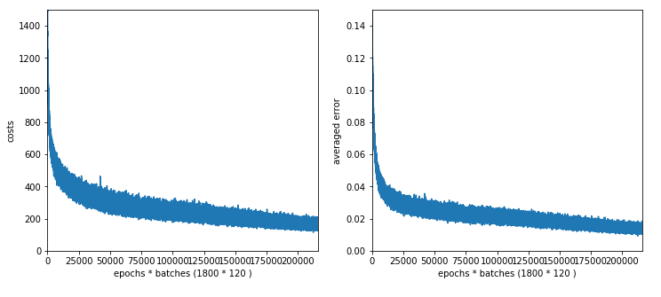
Regarding the use of different metrics for different tasks see machinelearningmastery.com / custom-metrics-deep-learning-keras-python/. In case of a classification problem, we are interested in the categorical “accuracy”. A metric can be monitored during training and will be recorded (besides aother data). We can use it for plotting information on the training process (a topic of the next article).

Training

Training is done by a function model.fit() – here: cnn.fit(). This function accepts a variety of parameters explained here: https://keras.io/ api/ models/ model_training_apis/ #fit-method.

We now can combine compilation and training in one function:

# Training 
def train( cnn, build=False, train_imgs, train_labels, reset, epochs, batch_size, optimizer, loss, metrics,
           li_Conv, li_Poo, li_MLP, input_shape ):
    if build:
        cnn = build_cnn_simple( li_Conv, li_Pool, li_MLP, input_shape)
        cnn.compile(optimizer=optimizer, loss=loss, metrics=metrics)        
        cnn.save_weights('cnn_weights.h5') # save the initial weights 
    # reset weights
    if reset and not build:
        cnn.load_weights('cnn_weights.h5')
    start_t = time.perf_counter()
    cnn.fit(train_imgs, train_labels, epochs=epochs, batch_size=batch_size, verbose=1, shuffle=True) 
    end_t = time.perf_counter()
    fit_t = end_t - start_t
    return cnn, fit_t  # we return cnn to be able to use it by other functions

Note that we save the initial weights to be able to load them again for a new training – otherwise Keras saves the weights as other model data after training and continues with the last weights found. The latter can be reasonable if you want to continue training in defined steps. However, in our forthcoming tests we repeat the training from scratch.

Keras offers a “save”-model and methods to transfer data of a CNN model to files (in two specific formats). For saving weights the given lines are sufficient. Hint: When I specify no path to the file “cnn_weights.h5” the data are – at least in my virtual Python environment – saved in the directory where the notebook is located.

First test

In a further Jupyter cell we place the following code for a test run:

  
# Perform a training run 
# ********************
build = False     
if cnn == None:
    build = True
batch_size=64
epochs=5
reset = True # we want training to start again with the initial weights

optimizer='rmsprop' 
loss='categorical_crossentropy'
metrics=['accuracy']

li_conv_1   = [32, (3,3), 0] 
li_conv_2   = [64, (3,3), 0] 
li_conv_3   = [64, (3,3), 0] 
li_Conv     = [li_conv_1, li_conv_2, li_conv_3]
li_pool_1   = [(2,2)]
li_pool_2   = [(2,2)]
li_Pool     = [li_pool_1, li_pool_2]
li_dense_1  = [70, 0]
li_dense_2  = [10, 0]
li_MLP      = [li_dense_1, li_dense_2]
input_shape = (28,28,1)

try: 
    if gpu:
        with tf.device("/GPU:0"):
            cnn, fit_time = train( cnn, build, train_imgs, train_
labels, 
                                   reset, epochs, batch_size, optimizer, loss, metrics, 
                                   li_Conv, li_Pool, li_MLP, input_shape)
        print('Time_GPU: ', fit_time)  
    else:
        with tf.device("/CPU:0"):
            cnn, fit_time = train( cnn, build, train_imgs, train_labels, 
                                   reset, epochs, batch_size, optimizer, loss, metrics, 
                                   li_Conv, li_Pool, li_MLP, input_shape)
        print('Time_CPU: ', fit_time)  
except SystemExit:
    print("stopped due to exception")

You recognize the parameterization of our train()-function. What results do we get ?

Epoch 1/5
60000/60000 [==============================] - 4s 69us/step - loss: 0.1551 - accuracy: 0.9520
Epoch 2/5
60000/60000 [==============================] - 4s 69us/step - loss: 0.0438 - accuracy: 0.9868
Epoch 3/5
60000/60000 [==============================] - 4s 68us/step - loss: 0.0305 - accuracy: 0.9907
Epoch 4/5
60000/60000 [==============================] - 4s 69us/step - loss: 0.0227 - accuracy: 0.9931
Epoch 5/5
60000/60000 [==============================] - 4s 69us/step - loss: 0.0184 - accuracy: 0.9948
Time_GPU:  20.610678611003095


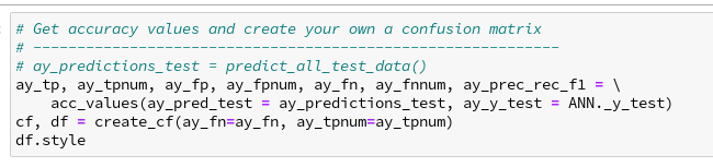
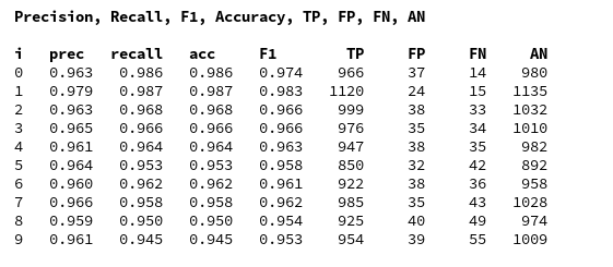
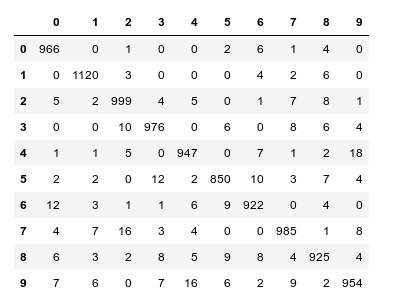
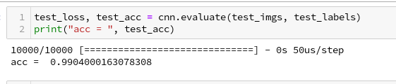
And a successive check on the test data gives us:

We can ask Keras also for a description of the model:

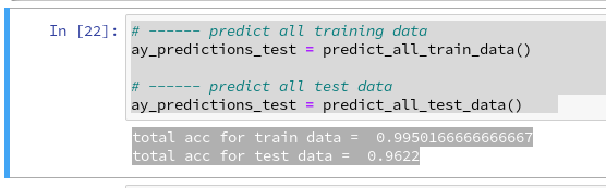
Accuracy at the 99% level

We got an accuracy on the test data of 99%! With 5 epochs in 20 seconds – on my old GPU.
This leaves us a very good impression – on first sight …

Conclusion

We saw today that it is easy to set up a CNN. We used a simple MLP to solve the problem of classification; the data to its input layer are provided by the output of the last convolutional layer. The tensor there has just to be “flattened”.

The level of accuracy reached is impressing. Well, its also a bit frustrating when we think about the efforts we put into our MLP, but we also get a sense for the power and capabilities of CNNs.

In the next post
A simple CNN for the MNIST dataset – III – inclusion of a learning-rate scheduler, momentum and a L2-regularizer
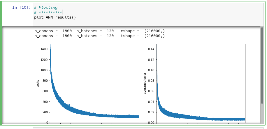
we will care a bit about plotting. We at least want to see the same accuracy and loss data which we used to plot at the end of our MLP tests.


MLP, Numpy, TF2 – performance issues – Step I – float32, reduction of back propagation

In my last article in this blog I wrote a bit about some steps to get Keras running with Tensorflow 2 [TF2] and Cuda 10.2 on Opensuse Leap 15.1. One objective of these efforts was a performance comparison between two similar Multilayer Perceptrons [MLP] :

  • my own MLP programmed with Python and Numpy; I have discuss this program in another article series;
  • an MLP with a similar setup based on Keras and TF2

Not for reasons of a competition, but to learn a bit about differences. When and for what parameters do Keras/TF2 offer a better performance?
Another objective is to test TF-alternatives to Numpy functions and possible performance gains.

For the Python code of my own MLP see the article series starting with the following post:

A simple Python program for an ANN to cover the MNIST dataset – I – a starting point

But I will discuss relevant code fragments also here when needed.

I think, performance is always an interesting topic – especially for dummies as me regarding Python. After some trials and errors I decided to discuss some of my experiences with MLP performance and optimization options in a separate series of the section “Machine learning” in this blog. This articles starts with two simple measures.

A factor of 6 turns turns into a factor below 2

Well, what did a first comparison give me? Regarding CPU time I got a factor of 6 on the MNIST dataset for a batch-size of 500. Of course, Keras with TF2 was faster 🙂 . Devastating? Not at all … After years of dealing with databases and factors of up to 100 by changes of SQL-statements and indexing a factor of 6 cannot shock or surprise me.

The Python code was the product of an unpaid hobby activity in my scarce free time. And I am still a beginner in Python. The code was also totally unoptimized, yet – both regarding technical aspects and the general handling of forward and backward propagation. It also contained and still contains a lot of superfluous statements for testing. Actually, I had expected an even bigger factor.

In addition, some things between Keras and my Python programs are not directly comparable as I only use 4 CPU cores for Openblas – this gave me an optimum for Python/Numpy programs in a Jupyter environment. Keras and TF2 instead seem to use all available CPU threads (successfully) despite limiting threading with TF-statements. (By the way: This is an interesting point in itself. If OpenBlas cannot give them advantages what else do they do?)

A very surprising point was, however, that using a GPU did not make the factor much bigger – despite the fact that TF2 should be able to accelerate certain operations on a GPU by at least by a factor of 2 up to 5 as independent tests on matrix operations showed me. And a factor of > 2 between my GPU and the CPU is what I remember from TF1-times last year. So, either the CPU is better supported now or the GPU-support of TF2 has become worse compared to TF1. An interesting point, too, for further investigations …

An even bigger surprise was that I could reduce the factor for the given batch-size down to 2 by just two major, butsimple code changes! However, further testing also showed a huge dependency on the batch sizechosen for training – which is another interesting point. Simple tests show that we may even be able to reduce the performance factor further by

  • by using directly coupled matrix operations – if logically possible
  • by using the basic low-level Python API for some operations

Hope, this sounds interesting for you.

The reference model based on Keras

I used the following model as a reference
in a Jupyter environment executed on Firefox:

Jupyter Cell 1

 
# compact version 
# ****************
import time 
import tensorflow as tf
#from tensorflow import keras as K
import keras as K
from keras.datasets import mnist
from keras import models
from keras import layers
from keras.utils import to_categorical
from keras import regularizers
from tensorflow.python.client import device_lib
import os

# use to work with CPU (CPU XLA ) only 
os.environ["CUDA_VISIBLE_DEVICES"] = "-1"
# The following can only be done once - all CPU cores are used otherwise  
tf.config.threading.set_intra_op_parallelism_threads(4)
tf.config.threading.set_inter_op_parallelism_threads(4)

gpus = tf.config.experimental.list_physical_devices('GPU')
if gpus:
  try:
    tf.config.experimental.set_virtual_device_configuration(gpus[0], 
          [tf.config.experimental.VirtualDeviceConfiguration(memory_limit=1024)])
  except RuntimeError as e:
    print(e)
    
# if not yet done elsewhere 
#tf.compat.v1.disable_eager_execution()
#tf.config.optimizer.set_jit(True)
tf.debugging.set_log_device_placement(True)

use_cpu_or_gpu = 0 # 0: cpu, 1: gpu

# function for training 
def train(train_images, train_labels, epochs, batch_size, shuffle):
    network.fit(train_images, train_labels, epochs=epochs, batch_size=batch_size, shuffle=shuffle)

# setup of the MLP
network = models.Sequential()
network.add(layers.Dense(70, activation='sigmoid', input_shape=(28*28,), kernel_regularizer=regularizers.l2(0.01)))
#network.add(layers.Dense(80, activation='sigmoid'))
#network.add(layers.Dense(50, activation='sigmoid'))
network.add(layers.Dense(30, activation='sigmoid', kernel_regularizer=regularizers.l2(0.01)))
network.add(layers.Dense(10, activation='sigmoid'))
network.compile(optimizer='rmsprop', loss='categorical_crossentropy', metrics=['accuracy'])

# load MNIST 
mnist = K.datasets.mnist
(X_train, y_train), (X_test, y_test) = mnist.load_data()
# simple normalization
train_images = X_train.reshape((60000, 28*28))
train_images = train_images.astype('float32') / 255
test_images = X_test.reshape((10000, 28*28))
test_images = test_images.astype('float32') / 255
train_labels = to_categorical(y_train)
test_labels = to_categorical(y_test)


Jupyter Cell 2

# run it 
if use_cpu_or_gpu == 1:
    start_g = time.perf_counter()
    train(train_images, train_labels, epochs=35, batch_size=500, shuffle=True)
    end_g = time.perf_counter()
    test_loss, test_acc= network.evaluate(test_images, test_labels)
    print('Time_GPU: ', end_g - start_g)  
else:
    start_c = time.perf_counter()
    with tf.device("/CPU:0"):
        train(train_images, train_labels, epochs=35, batch_size=500, shuffle=True)
    end_c = time.perf_counter()
    test_loss, test_acc= network.evaluate(test_images, test_labels)
    print('Time_CPU: ', end_c - start_c)  

# test accuracy 
print('Acc:: ', test_acc)

Typical output – first run:

 
Epoch 1/35
60000/60000 [==============================] - 1s 16us/step - loss: 2.6700 - accuracy: 0.1939
Epoch 2/35
60000/60000 [==============================] - 0s 5us/step - loss: 2.2814 - accuracy: 0.3489
Epoch 3/35
60000/60000 [==============================] - 0s 5us/step - loss: 2.1386 - accuracy: 0.3848
Epoch 4/35
60000/60000 [==============================] - 0s 5us/step - loss: 1.9996 - accuracy: 0.3957
Epoch 5/35
60000/60000 [==============================] - 0s 5us/step - loss: 1.8941 - accuracy: 0.4115
Epoch 6/35
60000/60000 [==============================] - 
0s 5us/step - loss: 1.8143 - accuracy: 0.4257
Epoch 7/35
60000/60000 [==============================] - 0s 5us/step - loss: 1.7556 - accuracy: 0.4392
Epoch 8/35
60000/60000 [==============================] - 0s 5us/step - loss: 1.7086 - accuracy: 0.4542
Epoch 9/35
60000/60000 [==============================] - 0s 5us/step - loss: 1.6726 - accuracy: 0.4664
Epoch 10/35
60000/60000 [==============================] - 0s 5us/step - loss: 1.6412 - accuracy: 0.4767
Epoch 11/35
60000/60000 [==============================] - 0s 5us/step - loss: 1.6156 - accuracy: 0.4869
Epoch 12/35
60000/60000 [==============================] - 0s 5us/step - loss: 1.5933 - accuracy: 0.4968
Epoch 13/35
60000/60000 [==============================] - 0s 5us/step - loss: 1.5732 - accuracy: 0.5078
Epoch 14/35
60000/60000 [==============================] - 0s 5us/step - loss: 1.5556 - accuracy: 0.5180
Epoch 15/35
60000/60000 [==============================] - 0s 5us/step - loss: 1.5400 - accuracy: 0.5269
Epoch 16/35
60000/60000 [==============================] - 0s 5us/step - loss: 1.5244 - accuracy: 0.5373
Epoch 17/35
60000/60000 [==============================] - 0s 5us/step - loss: 1.5106 - accuracy: 0.5494
Epoch 18/35
60000/60000 [==============================] - 0s 5us/step - loss: 1.4969 - accuracy: 0.5613
Epoch 19/35
60000/60000 [==============================] - 0s 5us/step - loss: 1.4834 - accuracy: 0.5809
Epoch 20/35
60000/60000 [==============================] - 0s 5us/step - loss: 1.4648 - accuracy: 0.6112
Epoch 21/35
60000/60000 [==============================] - 0s 5us/step - loss: 1.4369 - accuracy: 0.6520
Epoch 22/35
60000/60000 [==============================] - 0s 5us/step - loss: 1.3976 - accuracy: 0.6821
Epoch 23/35
60000/60000 [==============================] - 0s 5us/step - loss: 1.3602 - accuracy: 0.6984
Epoch 24/35
60000/60000 [==============================] - 0s 5us/step - loss: 1.3275 - accuracy: 0.7084
Epoch 25/35
60000/60000 [==============================] - 0s 5us/step - loss: 1.3011 - accuracy: 0.7147
Epoch 26/35
60000/60000 [==============================] - 0s 5us/step - loss: 1.2777 - accuracy: 0.7199
Epoch 27/35
60000/60000 [==============================] - 0s 5us/step - loss: 1.2581 - accuracy: 0.7261
Epoch 28/35
60000/60000 [==============================] - 0s 5us/step - loss: 1.2411 - accuracy: 0.7265
Epoch 29/35
60000/60000 [==============================] - 0s 5us/step - loss: 1.2259 - accuracy: 0.7306
Epoch 30/35
60000/60000 [==============================] - 0s 5us/step - loss: 1.2140 - accuracy: 0.7329
Epoch 31/35
60000/60000 [==============================] - 0s 5us/step - loss: 1.2003 - accuracy: 0.7355
Epoch 32/35
60000/60000 [==============================] - 0s 5us/step - loss: 1.1890 - accuracy: 0.7378
Epoch 33/35
60000/60000 [==============================] - 0s 5us/step - loss: 1.1783 - accuracy: 0.7410
Epoch 34/35
60000/60000 [==============================] - 0s 5us/step - loss: 1.1700 - accuracy: 0.7425
Epoch 35/35
60000/60000 [==============================] - 0s 5us/step - loss: 1.1605 - accuracy: 0.7449
10000/10000 [==============================] - 0s 37us/step
Time_CPU:  11.055424336002034
Acc::  0.7436000108718872

 
A second run was a bit faster: 10.8 secs. Accuracy around: 0.7449.
The relatively low accuracy is mainly due to the regularization (and reasonable to avoid overfitting). Without regularization we would already have passed the 0.9 border.

My own unoptimized MLP-program was executed with the following parameter setting:


             my_data_set="mnist_keras", 
             n_hidden_layers = 2, 
             ay_nodes_layers = [0, 70, 30, 0], 
             n_nodes_layer_out = 10,
             num_test_records = 10000, # 
number of test data
             
             # Normalizing - you should play with scaler1 only for the time being      
             scaler1 = 1,   # 1: StandardScaler (full set), 1: Normalizer (per sample)        
             scaler2 = 0,   # 0: StandardScaler (full set), 1: MinMaxScaler (full set)       
             b_normalize_X_before_preproc = False,     
             b_normalize_X_after_preproc  = True,     

             my_loss_function = "LogLoss",
 
             n_size_mini_batch = 500,
             n_epochs = 35, 
             lambda2_reg = 0.01,  

             learn_rate = 0.001,
             decrease_const = 0.000001, 

             init_weight_meth_L0 = "sqrt_nodes",  # method to init weights in an interval defined by  =>"sqrt_nodes" or a constant interval  "const"
             init_weight_meth_Ln = "sqrt_nodes",  # sqrt_nodes", "const"
             init_weight_intervals = [(-0.5, 0.5), (-0.5, 0.5), (-0.5, 0.5)],   # in case of a constant interval
             init_weight_fact = 2.0,              # extends the interval 
             mom_rate   = 0.00005,

             b_shuffle_batches = True,    # shuffling the batches at the start of each epoch 
             b_predictions_train = True,  # test accuracy by  predictions for ALL samples of the training set (MNIST: 60000) at the start of each epoch
             b_predictions_test  = False,  
             prediction_train_period = 1, # 1: each and every epoch is used for accuracy tests on the full training set
             prediction_test_period = 1,  # 1: each and every epoch is used for accuracy tests on the full test dataset


People familiar with my other article series on the MLP program know the parameters. But I think their names and comments are clear enough.

With a measurement of accuracy based on a forward propagation of the complete training set after each and every epoch (with the adjusted weights) I got a run time of 60 secs.

With accuracy measurements based on error tracking for batches and averaging over all batches, I get 49.5 secs (on 4 CPU threads). So, this is the mentioned factor between 5 and 6.

(By the way: The test indicates some space for improvement on the “Forward Propagation” 🙂 We shall take care of this in the next article of this series – promised).

So, these were the references or baselines for improvements.

Two measures – and a significant acceleration

Well, let us look at the results after two major code changes. With a test of accuracy performed on the full training set of 60000 samples at the start of each epoch I get the following result :

------------------
Starting epoch 35

Time_CPU for epoch 35 0.5518779030026053
relative CPU time portions: shuffle: 0.05  batch loop: 0.58  prediction:  0.37
Total CPU-time:  19.065050211000198

learning rate =  0.0009994051838157095

total costs of training set   =  5843.522
rel. reg. contrib. to total costs =  0.0013737131

total costs of last mini_batch   =  56.300297
rel. reg. contrib. to batch costs =  0.14256112

mean abs weight at L0 :  0.06393985
mean abs weight at L1 :  0.37341583
mean abs weight at L2 :  1.302389

avg total error of last mini_batch =  0.00709
presently reached train accuracy   =  0.99072

-------------------
Total training Time_CPU:  19.04528829299714

With accuracy taken only from the error of a batch:

avg total error of last mini_batch =  0.00806
presently reached train accuracy   =  0.99194
-------------------
Total training Time_CPU:  11.331006342999899

Isn’t this good news? A time of 11.3 secs is pretty close to what Keras provides us with! (Well, at least for a batch size of 500). And with a better result regarding accuracy on my side – but this has to do with a probably different
handling of learning rates and the precise translation of the L2-regularization parameter for batches.

Plots:

How did I get to this point? As said: Two measures were sufficient.

A big leap in performance by turning to float32 precision

So far I have never cared too much for defining the level of precision by which Numpy handles arrays with floating point numbers. In the context of Machine Learning this is a profound mistake. on a 64bit CPU many time consuming operations can gain almost a factor of 2 in performance when using float 32 precision – if the programmers tweaked everything. And I assume the Numpy guys did it.

So: Just use “dtype=np.float32” (np means “numpy” which I always import as “np”) whenever you initialize numpy arrays!

For the readers following my other series: You should look at multiple methods performing some kind of initialization of my “MyANN”-class. Here is a list:

 
    def _handle_input_data(self): 
        .....
            self._y = np.array([int(i) for i in self._y], dtype=np.float32)
        .....
        self._X = self._X.astype(np.float32)
        self._y = self._y.astype(np.int32)
        .....
    def _encode_all_y_labels(self, b_print=True):
        .....
        self._ay_onehot = np.zeros((self._n_labels, self._y_train.shape[0]), dtype=np.float32)
        self._ay_oneval = np.zeros((self._n_labels, self._y_train.shape[0], 2), dtype=np.float32)
   
        .....
    def _create_WM_Input(self):
        .....
        w0 = w0.astype(dtype=np.float32)
        .....
    def _create_WM_Hidden(self):
        .....
            w_i_next = w_i_next.astype(dtype=np.float32)
        .....
    def _create_momentum_matrices(self):
        .....
            self._li_mom[i] = np.zeros(self._li_w[i].shape, dtype=np.float32)
        .....
    def _prepare_epochs_and_batches(self, b_print = True):
        .....
        self._ay_theta = -1 * np.ones(self._shape_epochs_batches, dtype=np.float32) 
        self._ay_costs = -1 * np.ones(self._shape_epochs_batches, dtype=np.float32) 
        self._ay_reg_cost_contrib = -1 * np.ones(self._shape_epochs_batches, dtype=np.float32) 
        .....
        self._ay_period_test_epoch     = -1 * np.ones(shape_test_epochs, dtype=np.float32) 
        self._ay_acc_test_epoch        = -1 * np.ones(shape_test_epochs, dtype=np.float32) 
        self._ay_err_test_epoch        = -1 * np.ones(shape_test_epochs, dtype=np.float32) 
        self._ay_period_train_epoch    = -1 * np.ones(shape_train_epochs, dtype=np.float32) 
        self._ay_acc_train_epoch       = -1 * np.ones(shape_train_epochs, dtype=np.float32) 
        self._ay_err_train_epoch       = -1 * np.ones(shape_train_epochs, dtype=np.float32) 
        self._ay_tot_costs_train_epoch = -1 * np.ones(shape_train_epochs, dtype=np.float32) 
        self._ay_rel_reg_train_epoch   = -1 * np.ones(shape_train_epochs, dtype=np.float32) 
        .....
        self._ay_mean_abs_weight = -10 * np.ones(shape_weights, dtype=np.float32) 
        .....
 
   def _add_bias_neuron_to_layer(self, A, how='column'):
        .....
            A_new = np.ones((A.shape[0], A.shape[1]+1), dtype=np.float32)
        .....
            A_new = np.ones((A.shape[0]+1, A.shape[1]), dtype=np.float32)
    .....


After I applied these changes the factor in comparison to Keras went down to 3.1 – for a batch size of 500. Good news after a first simple step!

Reducing the CPU time once more

The next step required a bit more thinking. When I went through further more detailed tests of CPU consumption for various steps during training I found that the error back propagation through the network required significantly more time than the forward propagation.

At first sight this seems to be logical. There are more operations to be done between layers – real matrix multiplications with np.dot() (or np.matmul()) and element-wise multiplications with the “*”-operation. See also my PDF on the basic math:
Back_Propagation_1.0_200216.

But this is wrong assumption: When I measured CPU times in detail I saw that such operations took most time when network layer L0 – i.e. the input layer of the MLP – got involved. This also seemed to be reasonable: the weight matrix is biggest there; the input layer of all layers has most neuron nodes.

But when I went through the code I saw that I just had been too lazy whilst coding back propagation:

 
    ''' -- Method to handle error BW propagation for a mini-batch --'''
    def _bw_propagation(self, 
                        ay_y_enc, li_Z_in, li_A_out, 
                        li_delta_out, li_delta, li_D, li_grad, 
                        b_print = True, b_internal_timing = False):
        
        # Note: the lists li_Z_in, li_A_out were already filled by _fw_propagation() for the present batch 
        
        # Initiate BW propagation - provide delta-matrices for outermost layer
        # *********************** 
        # Input Z at outermost layer E  (4 layers -> layer 3)
        ay_Z_E = li_Z_in[self._n_total_layers-1]
        # Output A at outermost layer E (was calculated by output function)
        ay_A_E = li_A_out[self._n_total_layers-1]
        
        # Calculate D-matrix (derivative of output function) at outmost the layer - presently only D_sigmoid 
        ay_D_E = self._calculate_D_E(ay_Z_E=ay_Z_E, b_print=b_print )
        
        # Get the 2 delta matrices for the outermost layer (only layer E has 2 delta-matrices)
        ay_delta_E, ay_delta_out_E = self._calculate_delta_E(ay_y_enc=ay_y_enc, ay_A_E=ay_A_E, ay_D_E=ay_D_E, b_print=b_print) 
        
        # add the matrices at the outermost layer to their lists ; li_delta_out gets only one element 
        idxE = self._n_total_layers - 1
        li_delta_out[idxE] = ay_delta_out_E # this happens only once
        li_delta[idxE]     = ay_delta_E
        li_D[idxE]         = ay_D_E
        li_grad[idxE]      = None    # On the outermost layer there is no gradient ! 
        
        # Loop over all layers in reverse direction 
        # ******************************************
        # index range of target layers N in BW direction (starting with E-1 => 4 layers -> layer 2))
        range_N_bw_layer = reversed(range(0, self._n_total_layers-1))   # must be -1 as the last element is not taken 
        
        # loop over layers 
        for N in range_N_bw_layer:
            
            # Back Propagation operations between layers N+1 and N 
            # *******************************************************
            # this method handles the special treatment of bias nodes in Z_in, too
            ay_delta_N, ay_D_N, ay_grad_
N = self._bw_prop_Np1_to_N( N=N, li_Z_in=li_Z_in, li_A_out=li_A_out, li_delta=li_delta, b_print=False )
            
            # add matrices to their lists 
            li_delta[N] = ay_delta_N
            li_D[N]     = ay_D_N
            li_grad[N]= ay_grad_N
       
        return

 
with the following key function:

 
    ''' -- Method to calculate the BW-propagated delta-matrix and the gradient matrix to/for layer N '''
    def _bw_prop_Np1_to_N(self, N, li_Z_in, li_A_out, li_delta):
        '''
        BW-error-propagation between layer N+1 and N 
        Inputs: 
            li_Z_in:  List of input Z-matrices on all layers - values were calculated during FW-propagation
            li_A_out: List of output A-matrices - values were calculated during FW-propagation
            li_delta: List of delta-matrices - values for outermost ölayer E to layer N+1 should exist 
        
        Returns: 
            ay_delta_N - delta-matrix of layer N (required in subsequent steps)
            ay_D_N     - derivative matrix for the activation function on layer N 
            ay_grad_N  - matrix with gradient elements of the cost fnction with respect to the weights on layer N 
        '''
        
        # Prepare required quantities - and add bias neuron to ay_Z_in 
        # ****************************
        
        # Weight matrix meddling between layers N and N+1 
        ay_W_N = self._li_w[N]
        # delta-matrix of layer N+1
        ay_delta_Np1 = li_delta[N+1]

        # !!! Add row (for bias) to Z_N intermediately !!!
        ay_Z_N = li_Z_in[N]
        ay_Z_N = self._add_bias_neuron_to_layer(ay_Z_N, 'row')
        
        # Derivative matrix for the activation function (with extra bias node row)
        ay_D_N = self._calculate_D_N(ay_Z_N)
        
        # fetch output value saved during FW propagation 
        ay_A_N = li_A_out[N]
        
        # Propagate delta
        # **************
        # intermediate delta 
        ay_delta_w_N = ay_W_N.T.dot(ay_delta_Np1)
        # final delta 
        ay_delta_N = ay_delta_w_N * ay_D_N
        # reduce dimension again (bias row)
        ay_delta_N = ay_delta_N[1:, :]
        
        # Calculate gradient
        # ********************
        #     required for all layers down to 0 
        ay_grad_N = np.dot(ay_delta_Np1, ay_A_N.T)
        
        # regularize gradient (!!!! without adding bias nodes in the L1, L2 sums) 
        ay_grad_N[:, 1:] += (self._li_w[N][:, 1:] * self._lambda2_reg + np.sign(self._li_w[N][:, 1:]) * self._lambda1_reg) 
        
        return ay_delta_N, ay_D_N, ay_grad_N


Now, look at the eventual code:

 
    ''' -- Method to calculate the BW-propagated delta-matrix and the gradient matrix to/for layer N '''
    def _bw_prop_Np1_to_N(self, N, li_Z_in, li_A_out, li_delta, b_print=False):
        '''
        BW-error-propagation between layer N+1 and N 
        .... 
        '''
        # Prepare required quantities - and add bias neuron to ay_Z_in 
        # ****************************
        
        # Weight matrix meddling between layers N and N+1 
        ay_W_N = self._li_w[N]
        ay_delta_Np1 = li_delta[N+1]

        # fetch output value saved during FW propagation 
        ay_A_N = li_A_out[N]

        # Optimization ! 
        if N > 0: 
            ay_Z_N = li_Z_in[N]
            # !!! Add intermediate row (for bias) to Z_N !!!
            ay_Z_N = self._add_bias_neuron_to_layer(ay_Z_N, 'row')
        
            # Derivative matrix for the activation function (with extra bias node 
row)
            ay_D_N = self._calculate_D_N(ay_Z_N)
        
            # Propagate delta
            # **************
            # intermediate delta 
            ay_delta_w_N = ay_W_N.T.dot(ay_delta_Np1)
            # final delta 
            ay_delta_N = ay_delta_w_N * ay_D_N
            # reduce dimension again 
            ay_delta_N = ay_delta_N[1:, :]
            
        else: 
            ay_delta_N = None
            ay_D_N = None
        
        # Calculate gradient
        # ********************
        #     required for all layers down to 0 
        ay_grad_N = np.dot(ay_delta_Np1, ay_A_N.T)
        
        # regularize gradient (!!!! without adding bias nodes in the L1, L2 sums) 
        if self._lambda2_reg > 0.0: 
            ay_grad_N[:, 1:] += self._li_w[N][:, 1:] * self._lambda2_reg 
        if self._lambda1_reg > 0.0: 
            ay_grad_N[:, 1:] += np.sign(self._li_w[N][:, 1:]) * self._lambda1_reg 
        
        return ay_delta_N, ay_D_N, ay_grad_N


You have, of course, detected the most important change:

We do not need to propagate any delta-matrices (originally coming from the error deviation at the output layer) down to layer 1!

This is due to the somewhat staggered nature of error back propagation – see the PDF on the math again. Between the first hidden layer L1 and the input layer L0 we only need to fetch the output matrix A at L0 to be able to calculate the gradient components for the weights in the weight matrix connecting L0 and L1. This saves us from the biggest matrix multiplication – and thus reduces computational time significantly.

Another bit of CPU time can be saved by calculating only the regularization terms really asked for; for my simple densely populated network I almost never use Lasso regularization; so L1 = 0.

These changes got me down to the values mentioned above. And, note: The CPU time for backward propagation then drops to the level of forward propagation. So: Be somewhat skeptical about your coding if backward propagation takes much more CPU time than forward propagation!

Dependency on the batch size

I should remark that TF2 still brings some major and remarkable advantages with it. Its strength becomes clear when we go to much bigger batch sizes than 500:
When we e.g. take a size of 10000 samples in a batch, the required time of Keras and TF2 goes down to 6.4 secs. This is again a factor of roughly 1.75 faster.
I do not see any such acceleration with batch size in case of my own program!

More detailed tests showed that I do not gain speed with a batch size over 1000; the CPU time increases linearly from that point on. This actually seems to be a limitation of Numpy and OpenBlas on my system.

Because , I have some reasons to believe that TF2 also uses some basic OpenBlas routines, this is an indication that we need to put more brain into further optimization.

Conclusion

We saw in this article that ML programs based on Python and Numpy may gain a boost by using only dtype=float32 and the related accuracy for Numpy arrays. In addition we saw that avoiding unnecessary propagation steps between the first hidden and at the input layer helps a lot.

In the next article of this series we shall look a bit at the performance of forward propagation – especially during accuracy tests on the training and test data set.

Further articles in this series

MLP, Numpy, TF2 – performance issues – Step II – bias neurons,
F- or C- contiguous arrays and performance

MLP, Numpy, TF2 – performance issues – Step III – a correction to BW propagation

A simple Python program for an ANN to cover the MNIST dataset – XIII – the impact of regularization

I continue with my growing series on a Multilayer perceptron and the MNIST dataset.

A simple Python program for an ANN to cover the MNIST dataset – XII – accuracy evolution, learning rate, normalization
A simple Python program for an ANN to cover the MNIST dataset – XI – confusion matrix
A simple Python program for an ANN to cover the MNIST dataset – X – mini-batch-shuffling and some more tests
A simple Python program for an ANN to cover the MNIST dataset – IX – First Tests
A simple Python program for an ANN to cover the MNIST dataset – VIII – coding Error Backward Propagation
A simple Python program for an ANN to cover the MNIST dataset – VII – EBP related topics and obstacles
A simple Python program for an ANN to cover the MNIST dataset – VI – the math behind the „error back-propagation“
A simple Python program for an ANN to cover the MNIST dataset – V – coding the loss function
A simple Python program for an ANN to cover the MNIST dataset – IV – the concept of a cost or loss function
A simple Python program for an ANN to cover the MNIST dataset – III – forward propagation
A simple Python program for an ANN to cover the MNIST dataset – II – initial random weight values
A simple Python program for an ANN to cover the MNIST dataset – I – a starting point

In the last article of the series we made some interesting experiences with the variation of the “leaning rate”. We also saw that a reasonable range for initial weight values should be chosen.

Even more fascinating was, however, the impact of a normalization of the input data on a smooth and fast gradient descent. We drew the conclusion that normalization is of major importance when we use the sigmoid function as the MLP’s activation function – especially for nodes in the first hidden layer and for input data which are on average relatively big. The reason for our concern were saturation effects of the sigmoid functions and other functions with a similar variation with their argument. In the meantime I have tried to make the importance of normalization even more plausible with the help of a a very minimalistic perceptron for which we can analyze saturation effects a bit more in depth; you get to the related article series via the following link:

A single neuron perceptron with sigmoid activation function – III – two ways of applying Normalizer

There we also have a look at other normalizers or feature scalers.

But back to our series on a multi-layer perceptron. You may have have asked yourself in the meantime: Why did he not check the impact of the regularization? Indeed: We kept the parameter Lambda2 for the quadratic regularization term constant in all experiments so far: Lambda2 = 0.2. So, the question about the impact of regularization e.g. on accuracy is a good one.

How big is the regularization term and how does it evolve during gradient decent training?

I add even one more question: How big is the relative contribution of the regularization term to the total loss or cost function? In our Python program for a MLP model we included a so called quadratic Ridge term:

Lambda2 * 0.5 * SUM[all weights**2], where bias nodes are excluded from the sum.

From various books on Machine Learning [ML] you just learn to choose the factor Lambda2 in the range between 0.01 and 0.1. But how big is the resulting term actually in comparison to the standard cost term, then, and how does the ratio between both terms evolve during gradient descent? What factors influence this ratio?

As we follow a training strategy based on mini-batches the regularization contribution was and is added up to the costs of each mini-batch. So its relative importance varies of course with the size of the mini-batches! Other factors which may also be of some importance – at least during the first epochs – could be the total number of weights in our network and the range of initial weight values.

Regarding the evolution during a converging gradient descent we know already that the total costs go down on the path to a cost minimum – whilst the weight values reach a stable level. So there is a (non-linear!) competition between the regularization term and the real costs of the “Log Loss” cost function! During convergence the relative importance of the regularization term may therefore become bigger until the ratio to the standard costs reaches an eventual constant level. But how dominant will the regularization term get in the end?

Let us do some experiments with the MNIST dataset again! We fix some common parameters and conditions for our test runs:
As we saw in the last article we should normalize the input data. So, all of our numerical experiments below (with the exception of the last one) are done with standardized input data (using Scikit-Learn’s StandardScaler). In addition initial weights are all set according to the sqrt(nodes)-rule for all layers in the interval [-0.5*sqrt(1/num_nodes), 0.5*sqrt(1/num_nodes)], with num_nodes meaning the number of nodes in a layer. Other parameters, which we keep constant, are:

Parameters: learn_rate = 0.001, decrease_rate = 0.00001, mom_rate = 0.00005, n_size_mini_batch = 500, n_epochs = 800.

I added some statements to the method for cost calculation in order to save the relative part of the regularization terms with respect to the total costs of each mini-batch in a Numpy array and plot the evolution in the end. The changes are so simple that I omit showing the modified code.

A first look at the evolution of the relative contribution of regularization to the total loss of a mini-batch

How does the outcome of gradient descent look for standardized input data and a Lambda2-value of 0.1?

Lambda2 = 0.1
Results: acc_train: 0.999 , acc_test: 0.9714, convergence after ca. 600 epochs

We see that the regularization term actually dominates the total loss of a mini-batch at convergence. At least with our present parameter setting. In comparisoin to the total loss of the full training set the contribution is of course much smaller and typically below 1%.

A small Lambda term

Let us reduce the regularization term via setting Lambda = 0.01. We expect its initial contribution to the costs of a batch to be smaller then, but this does NOT mean that the ratio to the standard costs of the batch automatically shrinks significantly, too:

Lambda2 = 0.01
Results: acc_train: 1.0 , acc_test: 0.9656, convergence after ca. 350 epochs

Note the absolute scale of the costs in the plots! We ended up at a much lower level of the total loss of a batch! But the relative dominance of regularization at the point of convergence actually increased! However, this did not help us with the accuracy of our MLP-algorithm on the test data set – although we perfectly fit the training set by a 100% accuracy.

In the end this is what regularization is all about. We do not want a total overfitting, a perfect adaption of the grid to the training set. It will not help in the sense of getting a better general accuracy on other input data. A Lambda2 of 0.01 is much too small in our case!

Slightly bigger regularization with Lambda2 = 0.2

So lets enlarge Lambda2 a bit:
Lambda2 = 0.2
Results: acc_train: 0.9946 , acc_test: 0.9728, convergence after ca. 700 epochs

We get an improved accuracy!

Two other cases with significantly bigger Lambda2

Lambda2 = 0.4
Results: acc_train: 0.9858 , acc_test: 0.9693, convergence after ca. 600 epochs

Lambda2 = 0.8
Results: acc_train: 0.9705 , acc_test: 0.9588, convergence after ca. 400 epochs

OK, but in both cases we see a significant and systematic trend towards reduced accuracy values on the test data set with growing Lambda2-values > 0.2 for our chosen mini-batch size (500 samples).

Conclusion

We learned a bit about the impact of regularization today. Whatever the exact Lambda2-value – in the end the contribution of a regularization term becomes a significant part of the total loss of a mini-batch when we approached the total cost minimum. However, the factor Lambda2 must be chosen with a reasonable size to get an impact of regularization on the final minimum position in the weight-space! But then it will help to improve accuracy on general input data in comparison to overfitted solutions!

But we also saw that there is some balance to take care of: For an optimum of generalization AND accuracy you should neither make Lambda2 too small nor too big. In our case Lambda2 = 0.2 seems to be a reasonable and good choice. Might be different with other datasets.

All in all studying the impact of a variation of achieved accuracy with the factor for a Ridge regularization term seems to be a good investment of time in ML projects. We shall come back to this point already in the next articles of this series.

In the next article

A simple Python program for an ANN to cover the MNIST dataset – XIV – cluster detection in feature space

we shall start to work on cluster detection in the feature space of the MNIST data before using gradient descent.