A simple CNN for the MNIST dataset – XII – filter visualization for maps of the first two convolutional layers

Posted on 27. October 2020 by eremo

In the last article of this series

A simple CNN for the MNIST dataset – XI – Python code for filter visualization and OIP detection
A simple CNN for the MNIST dataset – X – filling some gaps in filter visualization
A simple CNN for the MNIST dataset – IX – filter visualization at a convolutional layer
A simple CNN for the MNIST dataset – VIII – filters and features – Python code to visualize patterns which activate a map strongly
A simple CNN for the MNIST dataset – VII – outline of steps to visualize image patterns which trigger filter maps
A simple CNN for the MNIST dataset – VI – classification by activation patterns and the role of the CNN’s MLP part

I provided some code to create visualizations of “OIPs” (original input pattern). An OIP is a characteristic pattern in an input image to which a selected map of the deepest convolutional layer of CNN reacts strongly. Most of the patterns we found showed some overall large scale structure with sub-structures of smaller dimensions. In many cases the patterns were repeated two or even more times with some spatial distance across the images’s surface. That we got unique and relatively big patterns for the last and deepest Conv layer is not surprising because the maps of this layer cover the original image area with just a few neurons, i.e. with coarse resolution. The related convolutional filters work across relatively large distances. The astonishing ability of deeper layers to detect unique large scale patterns in input images is based on the weighted superposition of filters working on smaller scales together with a reduction of resolution.

To get images of OIPs we fed the trained CNN with input images whose pixel values were statistically distributed. We optimized the pixel values of the input images for a maximum response of selected maps of the third, i.e. deepest convolutional layer. We can, however, apply the same methods also to maps of the first and the second convolutional layers of our CNN. Then we get much simpler patterns – in the sense of repetitions of many small scale elements.

Below I just provide images of OIPs triggering maps of the first two convolution layers without much further comments. I refer to the layer names as discussed in previous articles of this series.

Input image patterns which lead to a maximum activation of the maps of the convolutional layer Conv2D-1

Layer “Conv2D-1” has 32 maps. With simple fluctuations on the length scale of one to two pixels, we can easily create OIP-images for each of the maps.

Most of these images were actually derived from one and the same input image.

Input image patterns which lead to a maximum
activation of the maps of the convolutional layer Conv2D-2

Layer “Conv2D-2” has 32 maps. With simple fluctuations on the length scale of one to two pixels plus some experiments with pixel value fluctuation son longer scales, I could produce OIP-images for we can easily create OIP-images for 51 of the maps. Experiments for the other 13 maps took to long time; the systematic approach with large scale fluctuations, which we discussed thoroughly in previous articles did not help on layer 2. If you look at the images below, you see that it i more likely that we need specific short and middle-scale fluctuations. However, the amount of possible data combinations is just too big for a systematic investigation.

Conclusion

In the course of the last articles we got a nice overview over the kind of patterns to which the maps of the different convolutional layers of a CNN react to. We are well prepared now to turn back to the question of what the ominous “features” of objects in input images really are. In the meantime have a look at another application of filter visualization in the realm of Deep Dreams, which I recently started to discuss in another article series of this blog. Stay tuned and wear masks to avoid the Corona virus! Stay healthy!

Other (previous) articles in this series

A simple CNN for the MNIST dataset – IV – Visualizing the activation output of convolutional layers and maps
A simple CNN for the MNIST dataset – III – inclusion of a learning-rate scheduler, momentum and a L2-regularizer
A simple CNN for the MNIST datasets – II – building the CNN with Keras and a first test
A simple CNN for the MNIST datasets – I – CNN basics

Deep Dreams of a CNN trained on MNIST data – I – a first approach based on one selected map of a convolutional layer

Posted on 26. October 2020 by eremo

It is fun to play around with Convolutional Neural Networks [CNNs] on the level of an dedicated amateur. One of the reasons is the possibility to visualize the output of elementary building blocks of this class of AI networks. The resulting images help to understand CNN algorithms in an entertaining way – at least in my opinion. The required effort is in addition relatively limited: You must be willing to invest a bit of time into programming, but on a quite modest level of difficulty. And you can often find many basic experiments which are in within the reach of limited PC capabilities.

A special area where the visualization of CNN guided processes is the main objective is the field of “Deep Dreams“. Anyone studying AI methods sooner or later stumbles across the somewhat psychedelic, but none the less spectacular images which Google presented in 2016 as a side branch of their CNN research. Today, you can download DeepDream generators from GitHub.

When I read a bit more about “DeepDream” experiments, I quickly learned that people use quite advanced CNN architectures, like Google’s Inception CNNs, and apply them to high resolution images (see e.g. the Book of F. Chollet on “Deep Learning with Keras and Python” and ai.googleblog.com, 2015, inceptionism-going-deeper-into-neural). Even if you pick up an already trained version of an Inception CNN, you need some decent GPU power to do your own experiments. Another questionable point for an interested amateur is: What does one actually learn from applying “generators”, which others have programmed, and what from just following a “user guide” without understanding what a DeepDream SW actually does? Probably not much, even if you produce stunning images after some time…

So, I asked myself: Can one study basic methods of the DeepDream technology with self programmed tools and a simple dataset? Could one create a “DeepDream” visualization with a rather simply structured CNN trained on MNIST data?
The big advantage of the MNIST data set is that the individual samples are small; and the amount of numerical operations, which a related simple CNN must perform on input images, fits well to the capabilities of PC technology – even if the latter is some years old.

After a first look into DeepDream algorithms, I think: Yes, it should be possible. In a way DeepDream experiments are a natural extension of the visualization of CNN filters and maps which I have already discussed in depth in another article series. Therefore, DeepDream visualizations might even help us to better understand how the internal filter of CNNs work and what “features” are. However, regarding the creation of spectacular images we need to reduce our expectations to a reasonably low level:

A CNN trained on MNIST data works with gray images, low resolution and only simple feature patterns. Therefore, we will never produce such impressive images as published by DeepDream artists or by Google. But, we do have a solid chance to grasp some basic principles and ideas of this side-branch of AI with very simplistic tools.

As always in this blog, I explore a new field step-wise and let you as a reader follow me through the learning process. Throughout most of this new series of articles we will use a CNN created with the help of Keras and filter visualization tools which were developed in another article series of this blog. The CNN has been trained on the MNIST data set already.

In this first post we are going to pick just a single selected feature or response map of a deep CNN layer and let it “dream” upon a down-scaled image of roses. Well, “dream“, as a matter of fact, is a misleading expression; but this is true for the whole DeepDream
business – as we shall see. A CNN does not dream; “DeepDream” creation is more to be seen as an artistic discipline using algorithmic image enhancement.

The input image which we shall feed into our CNN today is shown below:

As our CNN works on a resolution level of 28×28 pixels, only, the “dreaming” will occur in a coarse way, very comparable to hallucinations on the blurred vision level of a short-sighted, myopic man. More precisely: Of a disturbed myopic man who works the whole day with images of digits and lets this poor experience enter and manipulate his dreamy visions of nicer things :-).

Actually, the setup for this article’s experiment was a bit funny: I got the input picture of roses from my wife, who is very much interested in art and likes flowers. I am myopic and in my soul still a theoretical physicist, who is much more attracted by numbers and patterns than by roses – if we disregard the interesting fractal nature of rose blossoms for a second :-).

What do DeepDreams based on single maps of trained MNIST CNNs produce?

To rouse your interest a bit or to disappoint you from the start, I show you a typical result of today’s exercise: “Dreams” or “hallucinations” based on MNIST and a selected single map of a deep convolutional CNN layer produce gray scale images with ghost-like “apparitions”.

When these images appeared on my computer screen, I thought: This is fun, indeed! But my wife just laughed – and said “physicists” with a known undertone and something about “boys and toys” …. I hope this will not stop you from reading further. Later articles will, hopefully, produce more “advanced” hallucinations. But as I said: It all depends on your expectations.

But, lets focus: How did I create the simple “dream” displayed above?

Requirements – a CNN and analysis and visualization tools described in another article series of this blog

I shall use results and methods, which I have already explained in another article series. You need a basic understanding of how a CNN works, what convolutional layers, kernel based filters and cost functions are, how we can build simple CNNs with the help of Keras, … – otherwise you will be lost from the beginning.
A simple CNN for the MNIST datasets – I – CNN basics
We also need a CNN, already trained on the MNIST data. I have shown how to build and train a very simple, yet suitable CNN with the help of Keras and Python; see e.g.:
A simple CNN for the MNIST datasets – II – building the CNN with Keras and a first test
A simple CNN for the MNIST dataset – III – inclusion of a learning-rate scheduler, momentum and a L2-regularizer
In addition we need some
code to create input image patterns which trigger response maps or full layers of a CNN optimally. I called such pixel patterns “OIPs”; others call them “features”. I have offered a Python class in the other article series which offers an optimization loop and other methods to work on OIPs and filter visualization.
A simple CNN for the MNIST dataset – XI – Python code for filter visualization and OIP detection

We shall extend this class by further methods throughout our forthcoming work. To develop and run the codes you should have a working Jupyter environment, a virtual Python environment, an IDE like Eclipse with PyDev for building larger code segments and a working Cuda installation for a NVidia graphics card. My 960GTX proved to be fully sufficient for what we are going to do.

Deep “Dream” – or some funny image manipulation?

As it unfortunately happens so often with AI topics: Also in case of the term “DeepDream” the vocabulary is exaggerated and thoroughly misleading. A simple CNN neither thinks nor “dreams” – it is a software manifestation of the results of an optimization algorithm applied to and trained on selected input data. If applied to new input, it will only detect patterns for which it was optimized before. You could also say:

A CNN is a manifestation of learned prejudices.

CNNs and other types of AI networks filter input according to encoded rules which serve a specific purpose and which reflect the properties of the selected training data set. If you ever used the CNN of my other series on your own hand-written images after a training only on the (US-) MNIST images you will quickly see what I mean. The MNIST dataset reflects an American style of writing digits – a CNN trained on MNIST will fail relatively often when confronted with image samples of digits written by Europeans.

Why do I stress this point at all? Because DeepDreams reveal such kinds of “prejudices” in a visible manner. DeepDream technology extracts and amplifies patterns within images, which fit the trained filters of the involved CNN. F. Chollet correctly describes “DeepDream” as an image manipulation technique which makes use of algorithms for the visualization of CNN filters.

The original algorithmic concept for DeepDreams consists of the following steps:

Extend your algorithm for CNN filter visualization (= OIP creation) from a specific map to the optimization of the response of complete layers. Meaning: Use the total response of all maps of a layer to define contributions to your cost function. Then mix these contributions in a defined weighted way.
Take some image of whatever motive you like and prepare 4 or more down-scaled versions of this image, i.e. versions with different levels of size and resolution below the original size and resolution.
Offer the image with the lowest resolution to the CNN as an input image.
Loop over all prepared image sizes :
- Apply your algorithm for filter visualization of all maps and layers to the input image – but only for a very limited amount of epochs.
- Upscale the resulting output image (OIP-image) to the next level of higher resolution.
- Add details of the original image with the same resolution to the upscaled OIP-image.
- Offer the resulting image as a new input image to your CNN.

Readers who followed me through my last series on “a simple CNN for MNIST” should already raise their eyebrows: What if the CNN expects a certain fixed size of of the input image? Well, a good question. I’ll come back to it in a second. For the time being, let us say that we will concentrate more on resolution than on an
actual image size.

The above steps make it clear that we manipulate an image multiple times. In a way we transform the image slowly to improve a layer’s response and repeat the process with growing resolution. I.e., we apply pattern detection and amplification on more and more details – in the end using all available large and small scale filters of the CNN in a controlled way without fully eliminating the original contents.

What to do about the low resolution of MNIST images and the limited capability of a CNN trained on them?

MNIST images have a very low resolution, real images instead a significantly higher one. With our CNN specialized on MNIST input the OIP-creation algorithm only works on (28×28)-images (and with some warnings, maybe, on smaller ones). What to do about it when we work with input images of a size of e.g. 560×560 pixels?

Well, we just work on the given level of resolution! We have three options:

We can downsize the input image itself or parts of it to the MNIST dimensions – with the help of a bicubic interpolation. Then our OIP-algorithm has the chance to detect OIPs on the coarse scale and to change the downsized image accordingly. Then we can upscale the result again to the original image size – and add details again.
We can split the input image into tiles of size (28×28) and offer these tiles as input to the CNN.
We can combine both of the above options.

Its like what a shortsighted human would do: Work with a blurred impression of the full scale image or look at parts of it from a close distance and then reassemble his/her impressions to larger scales.

A first step – apply only one specific map of a convolutional layer on a down-scaled image version

In this article we have a very limited goal for which we do not have to change our tools, yet:

Preparation:
- We choose a map.
- We downscale the original image to (28×28) by interpolation, upscale the result again by interpolating again (with loss) and calculate the difference to the original full resolution image (all interpolations done in a bicubic way).
Loop (4 times or so):
- We apply the OIP-algorithm on the downscaled input image for a fixed amount of epochs
- We upscale the result by bicubic interpolation to the original size.
- We re-add the difference in details.
- We downscale the result again.

With this approach I try to apply some of the elements of the original algorithm – but just on one scale of coarse resolution. I shall discuss the code for realizing the recipe given above with Python and Jupyter in the next article. For today let us look at some of the ghost like apparitions in the dreams for selected maps of the 3rd convolutional layer; see:
A simple CNN for the MNIST dataset – IX – filter visualization at a convolutional layer

DeepDreams based on selected maps of the 3rd convolutional layer of a CNN trained on MNIST data

With the image sections displayed below I have tried to collect results for different maps which focus on certain areas of the input image (with the exception of the first image section).

The first two images of each row display the detected OIP-patterns on the (28×28) resolution level with pixel values encoded in a (viridis) color-map; the third image in gray scale. The fourth image reveals the dream on the blurry vision level – up-scaled and interpolated to the original image size. You may still detect traces of the original rose blossoms i these images. The last two images of each row display the results
after re-adding details of the original image and an adjustment of the width of the value distribution. The detected and enhanced pattern then turns into a whitey, ghostly shadow.

I have given each section a fancy headline.

I never promised you a rose garden …

“Getting out …”

“Donut …”

“Curls to form a 3 …”

“Two of them …”

“The creepy roots of it all …”

“Look at me …”

“A hidden opening …”

“Soft is something different …”

“Central separation …”

Conclusion: A CNN
detects patterns or parts of patterns it was trained for in any kind of offered input …

You can compare the results to some input patterns (OIPs) which strongly trigger individual maps on the 3rd convolutional layer; you will detect similarities. E.g. four OIP- or feature patterns to which map 56 reacts strongly, look like:

This explains the basic shape of the “apparition” in the first “dream”:

This proves that the filters of a trained CNN actually detect patterns, which proved to be useful for a certain training purpose, in any kind of input which shows some traces of such patterns. A CNN simply does not “know” better: If you only have a hammer to interact with the world, everything becomes a nail to you in the end – this is the level of stupidity on which a CNN algorithm works. And it actually is a fundamental ingredient of DeepDream image manipulation – a transportation of learned patterns or prejudices to an environment outside the original training context.

In the next article
Deep Dreams of a CNN trained on MNIST data – II – some code for pattern carving
I provide the code for creating the above images.

Further articles in this series

Deep Dreams of a CNN trained on MNIST data – II – some code for pattern carving
Deep Dreams of a CNN trained on MNIST data – III – catching dream patterns at smaller length scales

A simple CNN for the MNIST dataset – XI – Python code for filter visualization and OIP detection

Posted on 18. October 2020 by eremo

I continue my article series on a CNN for the MNIST dataset and related studies of a CNN’s reaction to input patterns.

A simple CNN for the MNIST dataset – X – filling some gaps in filter visualization
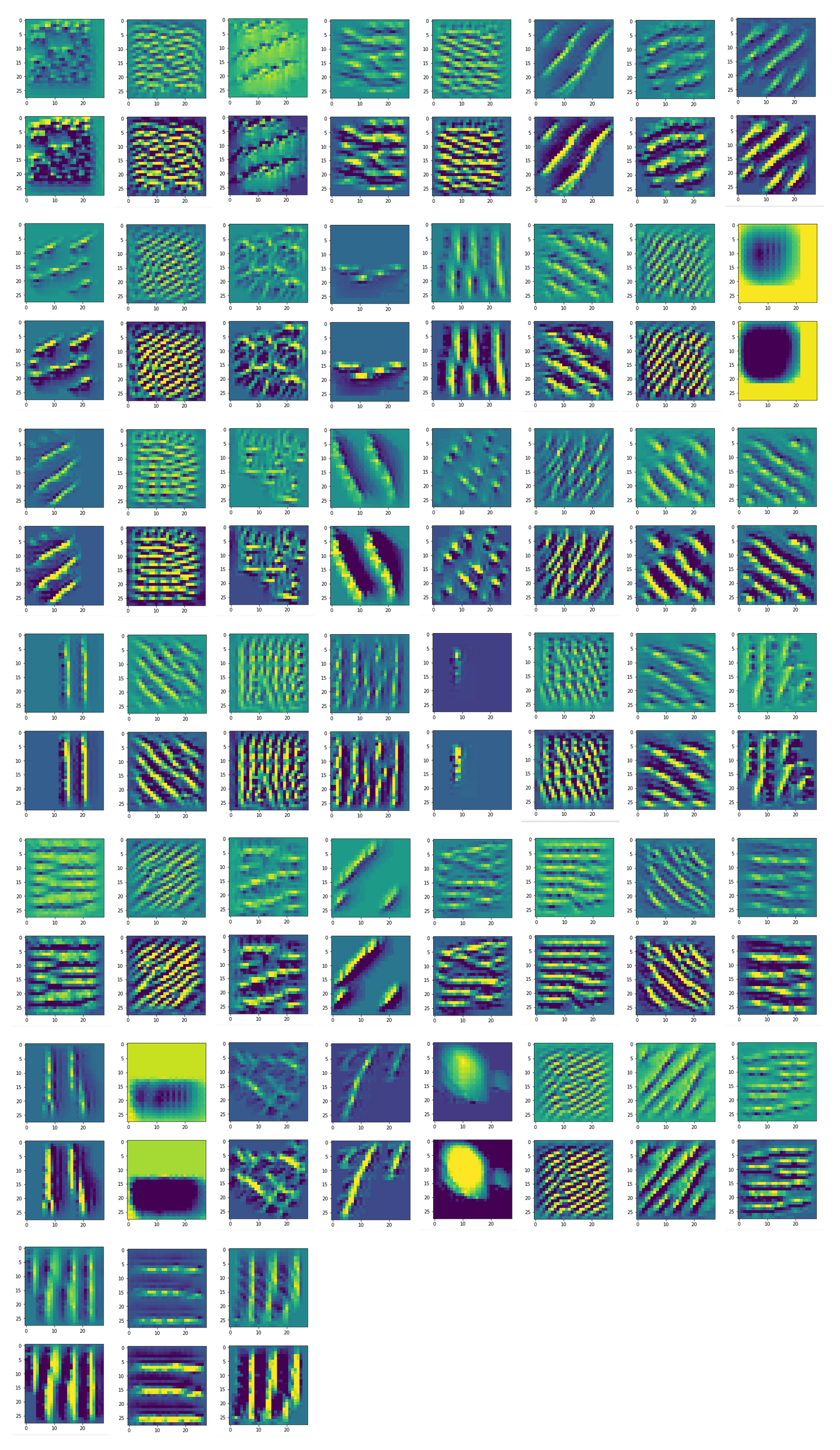
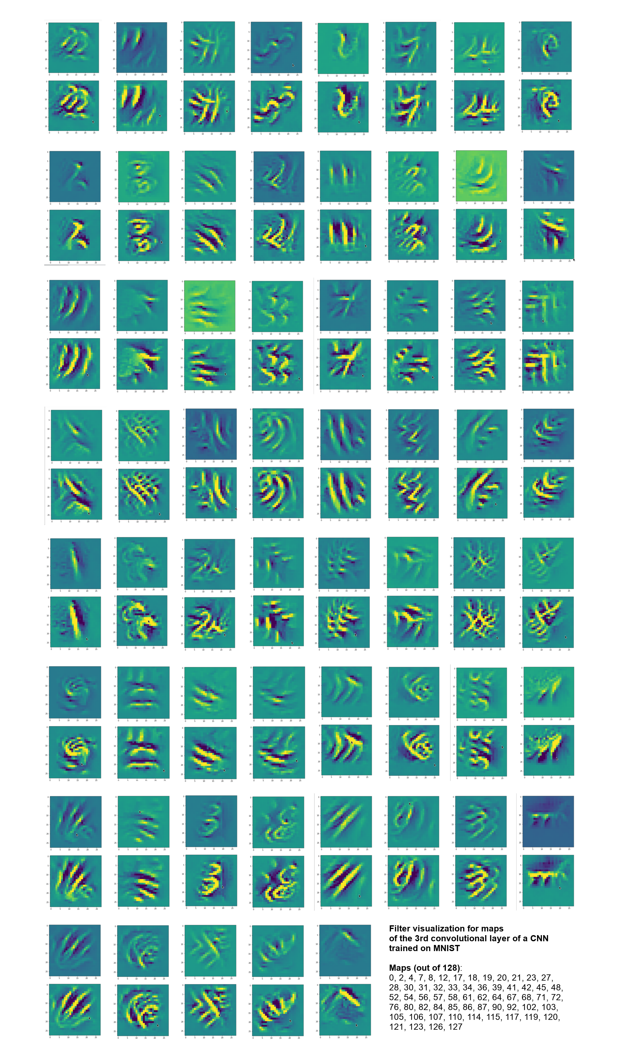
A simple CNN for the MNIST dataset – IX – filter visualization at a convolutional layer
A simple CNN for the MNIST dataset – VIII – filters and features – Python code to visualize patterns which activate a map strongly
A simple CNN for the MNIST dataset – VII – outline of steps to visualize image patterns which trigger filter maps
A simple CNN for the MNIST dataset – VI – classification by activation patterns and the role of the CNN’s MLP part
A simple CNN for the MNIST dataset – V – about the difference of activation patterns and features

In the course of this series we have already seen that that we must distinguish carefully between

activation patterns resulting from the output of the maps of a convolutional layer
and pixel patterns (OIPs) within input images which trigger a strong reaction of a selected deep layer map.

OIPs are patterns which pass complicated filter combinations of a sequence of convolutional layers. The images I have showed you so far show: At deep layers some maps react to unique large scale patterns covering a significant area of the input image in one or both dimensions. The patterns may expose sub-structures and spatially shifted repetitions across the images’s surface.

We can display map activation patterns easily on a grid displaying all maps of a layer and their neuron activations. OIP patterns, however, must be made visible via an image whose pixel values are determined by a complicated calculation process: The image data come from an optimization algorithm which analyzes the activation response of a map’s neurons to pixel value changes.

Our hunt for interesting MNIST OIPs, which trigger the maps of the deepest convolutional layer, has been relatively successful over the last two blog posts: Simply assigning a random value to each input pixel as a starting point for our algorithm already gave us OIP patterns for around 48% of the maps. In the last article I discussed an additional method to fill some of the gaps: I suggested to systematically investigate long range fluctuations of the pixel values as an input to the optimization loop. This gave us OIPs for another 26% of the maps. So, we have found OIPs for around 75% of the 128 maps with relatively simple methods.

But I still owe my readers some code for OIP-creation and a short guideline how to use it. You find the complete code in the last section of this article. I have encapsulated the methods for producing OIP-patterns in a Python class named “My_OIP”. The code is commented and with the knowledge accumulated during the last articles of this series you should have no major difficulties to understand it. Below I shall provide you with additional code for a sequence of Jupyter cells and walk you through the usage of the class’ methods.

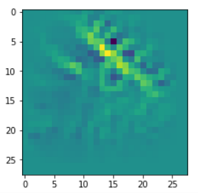
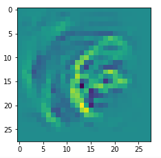
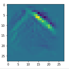
We are mostly interested in maps for which you do not get an OIP pattern (or a “feature”, if you like …) easily by trial and error methods. We therefore pick map Nr. 35 on layer “Conv2D_3” of my (!) trained CNN as an example.

Basic requirements and restrictions

I have tested the code only in combination with a sequence of Jupyter cells. So, you need both a virtual Python environment and a Jupyter installation to repeat my experiments.

The code is not yet build for a full investigation of all maps of a convolutional layer in one extensive run. The present methods are intended to be applied to a single selected map, only. Whenever you want to study another map you have to run a certain sequence of Jupyter cells again.

Another hint: I did all runs in a virtual Python environment with Tensorflow 2.2.1 as my Keras backend. Unfortunately, the code does not yet run as efficiently on TF 2.3.1 as on TF 2.2.1 for unclear reasons. I used the “Keras” version integrated into TF 2.

Required Modules

I invoke the following collection of Python modules:

Jupyter cell 1:

  
import numpy as np
from numpy import save
from numpy import load
import scipy
from itertools import product 
from sklearn.preprocessing import StandardScaler

import tensorflow as tf
from tensorflow import keras as K
from tensorflow.python.keras import backend as B 
#from tensorflow.keras import backend as B 
from tensorflow.keras import models
from tensorflow.keras import layers
from tensorflow.keras import regularizers
from tensorflow.keras import optimizers
from tensorflow.keras.optimizers import schedules
from tensorflow.keras.utils import to_categorical
from tensorflow.keras.datasets import mnist

from tensorflow.python.client import device_lib
#import tensorflow.contrib.eager as tfe

import matplotlib as mpl
from matplotlib import pyplot as plt
from matplotlib.colors import ListedColormap
import matplotlib.patches as mpat 

import time 
import sys 
import math
import os 
from os import path as path
import imp

# my own class code 
from mycode import myOIP
from mycode import myann32

from IPython.core.tests.simpleerr import sysexit

You may have to adjust some versions of these modules to get full consistency with TF 2.2.1. Watch the output of “pip-review” or “pip –upgrade –force” commands carefully! The general form of the required pip-statements to install a certain version of a module in your virtual Python environment looks like

pip install --upgrade --force tensorflow==2.2.1
pip install --upgrade --force six==1.12.0
pip install --upgrade --force bleach==1.5.0
....

Enable the code to run at least partially on a graphics card

A systematic investigation of long range fluctuation patterns as a starting point for an OIP-creation should be done with the help of a graphics card – it takes too much time to perform all of the required operations on the cores of a conventional CPU. [At least on my elderly equipment – unfortunately, I have no employer which sponsors my ML- and Linux-activities .. 🙁 ..] You can do the necessary preparatory steps with the help of a 2nd Jupyter cell.

Jupyter cell 2:

  
gpu = True
if gpu: 
    GPU = True;  CPU = False; num_GPU = 1; num_CPU = 4
else: 
    GPU = False; CPU = True;  num_CPU = 1; num_GPU = 0

config = tf.compat.v1.ConfigProto(intra_op_parallelism_threads=4,
                        inter_op_parallelism_threads=1, 
                        allow_soft_placement=True,
                        device_count = {'CPU' : num_CPU,
                                        'GPU' : num_GPU}, 
                        log_device_placement=True

config.gpu_options.per_process_gpu_memory_fraction=0.30
config.gpu_options.force_gpu_compatible = True
B.set_session(tf.compat.v1.Session(config=config))

I reduced the maximum usage of graphics card memory to 30% of its capacity (4GB).

Creating an object instance of the class My_OIP

As a third step we instantiate an object based on class “My_OIP”. When you look at the code of the class’ “__init__()”-method you see

that the my CNN-model is loaded from a h5-file and made available for further operations
and that an additional Keras model – named “OIP-(sub)-model” – is created. The OIP-model connects the input of the CNN with the output of the CNN’s innermost convolutional layer “Conv2D_3”. It is a sub-model of the original CNN.

The OIP-sub-model is built with the help of the “Model” class of Keras. At the end of the “__init__()”-method I print out the layer structures of the CNN- and OIP-model. The Juypter code is:

Jupyter cell 3:

# Load the CNN-model - build the OIP-model
#  ~~~~~~~~~~~~~~~~~~~~~~~~~~~~~~~~~~~~~~
imp.reload(myOIP)
try:
    with tf.device("/GPU:0"):
        MyOIP = myOIP.My_OIP(cnn_model_file = 'cnn_best.h5', layer_name = 'Conv2D_3')

except SystemExit:
    print("stopped")

Note that we chose a specific convolutional layer of the CNN, here, by providing its unique name as a parameter. When you look at the code you see that you can change the layer afterwards by directly calling method “_build_oip_model(layer_name = ‘LAYER_NAME’)” with a suitable name of the layer whose maps you want to study.

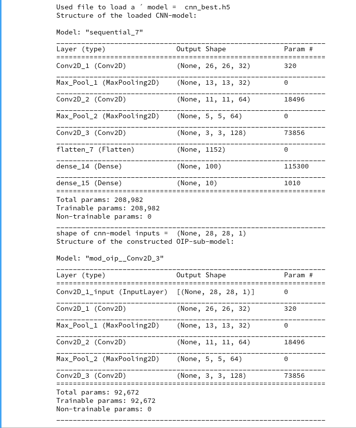
The resulting output looks in my case like

Used file to load a ´ model =  cnn_best.h5
Structure of the loaded CNN-model:

Model: "sequential_7"
_________________________________________________________________
Layer (type)                 Output Shape              Param #   
=================================================================
Conv2D_1 (Conv2D)            (None, 26, 26, 32)        320       
_________________________________________________________________
Max_Pool_1 (MaxPooling2D)    (None, 13, 13, 32)        0         
_________________________________________________________________
Conv2D_2 (Conv2D)            (None, 11, 11, 64)        18496     
_________________________________________________________________
Max_Pool_2 (MaxPooling2D)    (None, 5, 5, 64)          0         
_________________________________________________________________
Conv2D_3 (Conv2D)            (None, 3, 3, 128)         73856     
r
_________________________________________________________________
flatten_7 (Flatten)          (None, 1152)              0         
_________________________________________________________________
dense_14 (Dense)             (None, 100)               115300    
_________________________________________________________________
dense_15 (Dense)             (None, 10)                1010      
=================================================================
Total params: 208,982
Trainable params: 208,982
Non-trainable params: 0
_________________________________________________________________
shape of cnn-model inputs =  (None, 28, 28, 1)
Structure of the constructed OIP-sub-model:

Model: "mod_oip__Conv2D_3"
_________________________________________________________________
Layer (type)                 Output Shape              Param #   
=================================================================
Conv2D_1_input (InputLayer)  [(None, 28, 28, 1)]       0         
_________________________________________________________________
Conv2D_1 (Conv2D)            (None, 26, 26, 32)        320       
_________________________________________________________________
Max_Pool_1 (MaxPooling2D)    (None, 13, 13, 32)        0         
_________________________________________________________________
Conv2D_2 (Conv2D)            (None, 11, 11, 64)        18496     
_________________________________________________________________
Max_Pool_2 (MaxPooling2D)    (None, 5, 5, 64)          0         
_________________________________________________________________
Conv2D_3 (Conv2D)            (None, 3, 3, 128)         73856     
=================================================================
Total params: 92,672
Trainable params: 92,672
Non-trainable params: 0

You see that the OIP-model (“mod_oip__Conv2D_3”) starts with the input layer and ends with the output of the last deepest layer “Conv2D_3”.

Preparation and execution of a precursor-run

The code in the next Jupyter cell

first starts a method to prepare a precursor-run,
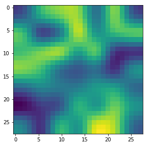
then defines a figure to allow for plots of the 8 promising input images with large scale fluctuations
and eventually starts a precursor-run which tests around 19800 fluctuation patterns and selects those 8, which trigger our selected map maximally.

What I call “precursor-run” above is, at its core, nothing else than a loop which tests a selected map’s response to many artificially created input images based on a variety of large scale fluctuations imposed on the pixel values.

Jupyter cell 4:

  
# preparation of the precursor run 
# ~~~~~~~~~~~~~~~~~~~~~~~~~~~~~~~
with tf.device("/GPU:0"):
    MyOIP._prepare_precursor(map_index=38)

# figure for plots
# -----------------
#sizing
fig_size = plt.rcParams["figure.figsize"]
fig_size[0] = 16
fig_size[1] = 8
fig_a = plt.figure()
axa_1 = fig_a.add_subplot(241)
axa_2 = fig_a.add_subplot(242)
axa_3 = fig_a.add_subplot(243)
axa_4 = fig_a.add_subplot(244)
axa_5 = fig_a.add_subplot(245)
axa_6 = fig_a.add_subplot(246)
axa_7 = fig_a.add_subplot(247)
axa_8 = fig_a.add_subplot(248)
li_axa = [axa_1, axa_2, axa_3, axa_4, axa_5, axa_6, axa_7, axa_8]

# start precursor run 
# ~~~~~~~~~~~~~~~~~~~~~~~~~~~~~~~
start_t = time.perf_counter()
with tf.device("/GPU:0"):
    MyOIP._precursor(num_epochs=10, li_axa=li_axa)
end_t   = time.perf_counter()
fit_t = end_t - start_t
print("time= ", fit_t)

Note that we define the map we which we want to test when we call “_prepare_precursor(map_index=38)”; the index of the map refers to its position in the list of maps of the chosen layer.

Technically, method “_prepare_precursor()” sets up the OIP-model for the selected map (here map 38) plus a GradientTape-object, which helps us to automatically calculate gradient component values for the map-output with respect to input pixel-values. It does so by calling method

_setup_gradient_tape_and_iterate_function() .

The latter method also creates the “_iterate()-function” which we use during the optimization of the input pixel values.

Method “_precursor()” then systematically creates input images for the fluctuation patterns originally imposed on a coarse (3×3)-grid by interpolating and upscaling. When you study the code carefully you will see that I included a possibility to overlay some kind of constant short scale fluctuation pattern. (This may prove useful in some cases where a map needs short and long scale input patterns at the same time to react with a reasonable activation.)

The method then loops over all long range patterns, performs a defined number of gradient ascent steps for each image and saves the respective pattern data if the map shows a reaction – indicated by a loss value > 0. The optimization loop is directly handled within the method for performance reasons. Note that we only follow the optimization process for a fixed, relatively small numbers of epochs. The loop prints out loss values for all patterns for which the loss is > 0.

In the end we select those 8 input images which showed the highest loss values and save their basic pattern data for reconstruction. The patterns are afterwards available in a list (“self._li_of_flucts”). (We save them also in a file).

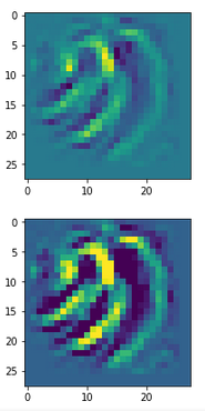
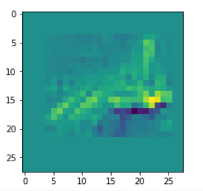
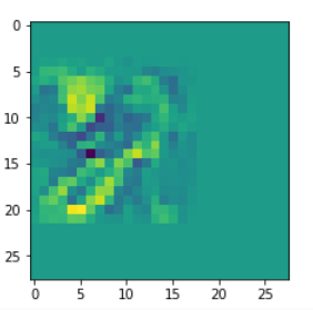
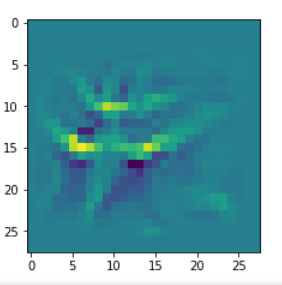
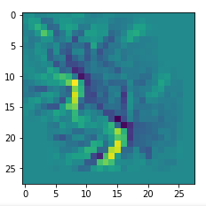
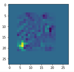
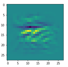
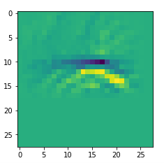
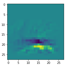
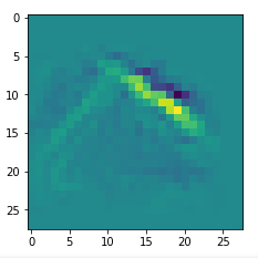
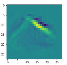
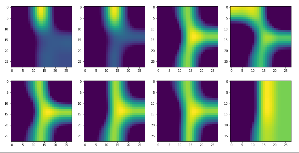
We then check whether the image reconstruction algorithm for one of the saved patterns really works. A final step consists of a display of the selected input images. We get an output that looks like

  
We test  19683  possibilities for a (3x3) fluctuations 
i =  27  loss =  5.528541
i =  28  loss =  3.826129
i =  30  loss =  5.545482
i =  31  loss =  5.8238125
i =  32  loss =  2.5444937
i =  36  loss =  2.7260687
i =  37  loss =  3.1436405
i =  46  loss =  2.8298864
i =  54  loss =  5.528542
i =  55  loss =  5.286209 
...
...
i =  19664  loss =  9.8695545
i =  19671  loss =  2.4347296
i =  19672  loss =  2.8202498
i =  19673  loss =  9.868241

num of relevant covs =  11114 
check of map reaction to first selected image
loss for 1st selected img =  20.427849
0 loss =  20.427849
1 loss =  19.50778
2 loss =  19.394796
3 loss =  18.993208
4 loss =  18.844856
5 loss =  18.794407
6 loss =  18.771235
7 loss =  18.607782
time=  251.3919793430032

The test of the fluctuation patterns for map 38 found 1114 candidates with a significant loss.

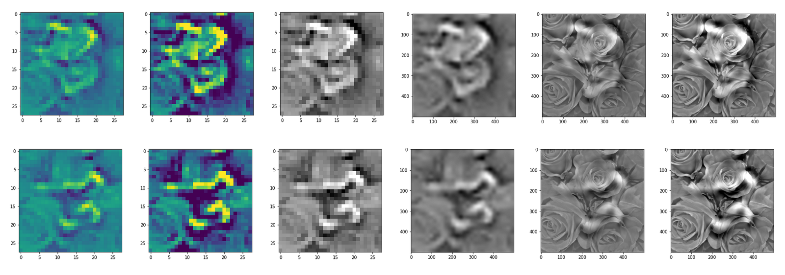
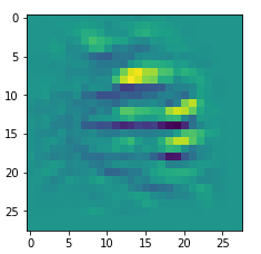
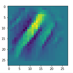
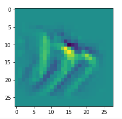
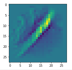
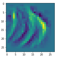
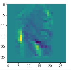
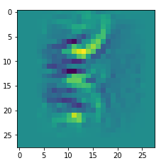
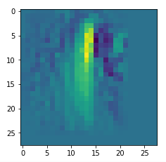
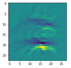
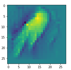
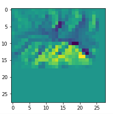
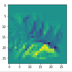
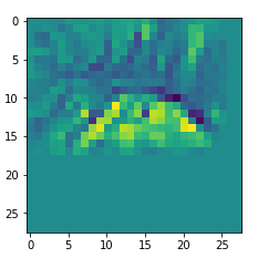
In my case the selected images of the 8 most promising pattern candidates for OIP-creation look like:

Reconstruction of the input image candidates from their fluctuation pattern

We can reconstruct the images from the contents of “self._li_of_flucts()” by calling method “_display_precursor_imgs()”.

Jupyter cell 5:

  
# figure
# -----------
#sizing
fig_size = plt.rcParams["figure.figsize"]
fig_size[0] = 16
fig_size[1] = 8
fig_a = plt.figure()
axa_1 = fig_a.add_subplot(241)
axa_2 = fig_a.add_subplot(242)
axa_3 = fig_a.add_subplot(243)
axa_4 = fig_a.add_subplot(244)
axa_5 = fig_a.add_
subplot(245)
axa_6 = fig_a.add_subplot(246)
axa_7 = fig_a.add_subplot(247)
axa_8 = fig_a.add_subplot(248)
li_axa = [axa_1, axa_2, axa_3, axa_4, axa_5, axa_6, axa_7, axa_8]

with tf.device("/GPU:0"):
    #MyOIP._display_imgs_2()    
    MyOIP._display_precursor_imgs(li_axa=li_axa)

It will test the reconstruction algorithm and display the 8 images already provided by the precursor run again.

Choose an input image candidate and enrich it by small scale fluctuations

The next Jupyter cell offers the opportunity to select a certain candidate out of our 8 candidates and create the respective input image as a basis for a subsequent OIP-creation. In addition it allows us to enrich its large scale fluctuation pattern with some small scale fluctuations at a lower “amplitude”. We must provide a figure with two subplots to do some plotting.

Jupyter cell 6:

 
# build initial image based on PRECURSOR
# *******************

# figure
# -----------
#sizing
fig_size = plt.rcParams["figure.figsize"]
fig_size[0] = 10
fig_size[1] = 5
fig1 = plt.figure(1)
ax1_1 = fig1.add_subplot(121)
ax1_2 = fig1.add_subplot(122)

try: 
    # OIP function to setup an initial image 
    with tf.device("/GPU:0"):
        
        initial_img = MyOIP._build_initial_img_from_prec( prec_index=7, 
                                             li_epochs    = [20, 50, 100, 400], 
                                             li_facts     = [1.0, 0.0, 0.0, 0.2, 0.0],
                                             li_dim_steps = [ (3,3), (7,7), (14,14), (28,28) ], 
                                             b_smoothing = False, b_display=True, 
                                             ax1_1 = ax1_1, ax1_2 = ax1_2)

except SystemExit:
    print("stopped")

Parameter “prec_index” reflects which of the eight long range fluctuation patterns you choose.

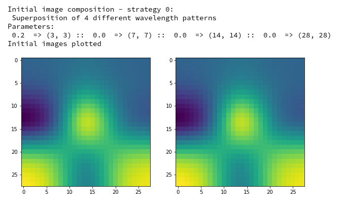
You certainly noticed the options for parameterizing additional fluctuations: “li_dim_steps” defines the granularity of the fluctuations which are upscaled to the (28×28)-size of the MNIST images. “li_facts” allows for a relative scaling of the strength of the fluctuations. Note that the first element of li_facts determines the strength of the chosen basic pattern after the “_precursor”-run; the other 4 parameters define the relative strength of the other statistical fluctuations on the four length-scales (li_dim_steps).

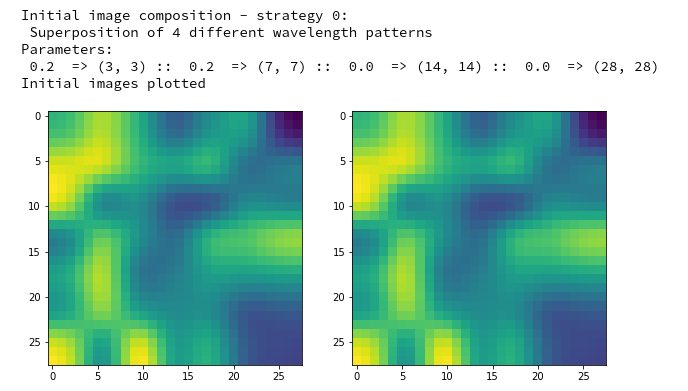
Let us look at an example:

initial_img = MyOIP._build_initial_img_from_prec( prec_index=7, 
  li_epochs    = [20, 50, 100, 400], 
  li_facts     = [1.0, 0.0, 0.0, 0.0, 0.0],
  li_dim_steps = [ (3,3), (7,7), (14,14), (28,28) ], 
  b_smoothing = False, b_display=True, 
  ax1_1 = ax1_1, ax1_2 = ax1_2)

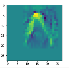
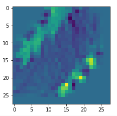
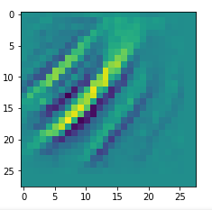
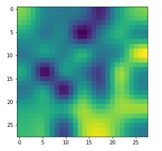
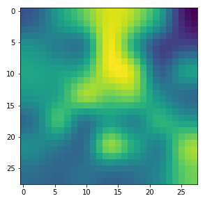
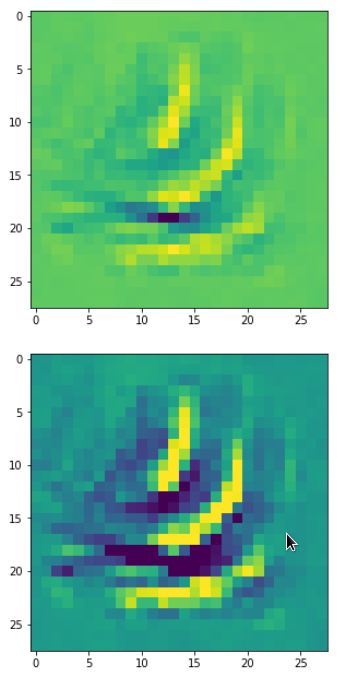
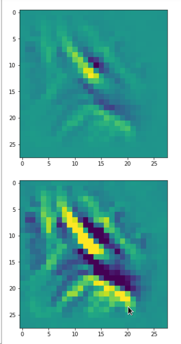
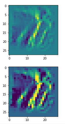
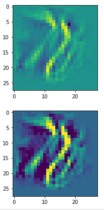
picks the last of the patterns displayed above as the results of the precursor run. The result looks like:

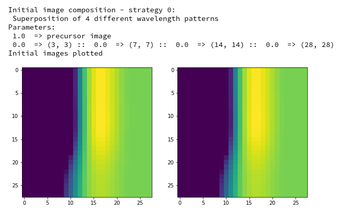
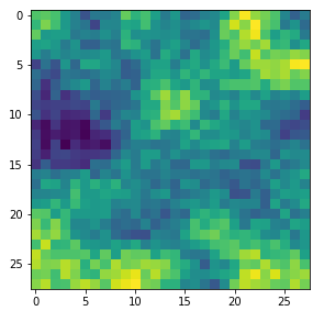
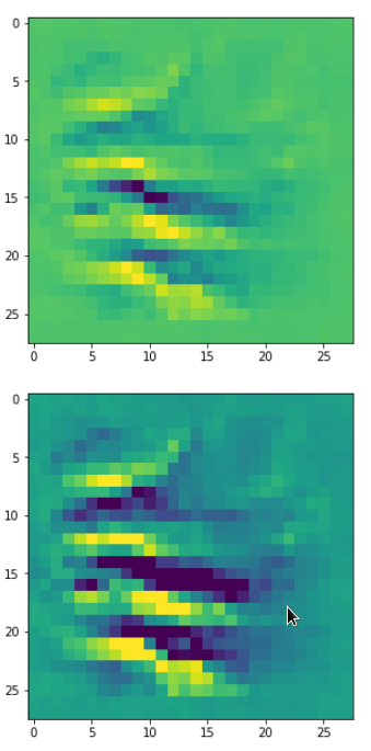
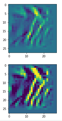
The second image should look like the first one – it is created for check purposes, only. Now, we enrich this image with fluctuations on the scale defined by (14,14), i.e. on squares of (2×2)-dimensions. (The MNIST image size is (28×28)!)

initial_img = MyOIP._build_initial_img_from_prec( prec_index=7, 
  li_epochs    = [20, 50, 100, 400], 
  li_facts     = [1.0, 0.0, 0.0, 0.2, 0.0],
  li_dim_steps = [ (3,3), (7,7), (14,14), (28,28) ], 
  b_smoothing = False, b_display=True, 
  ax1_1 = ax1_1, ax1_2 = ax1_2)

We get the result:

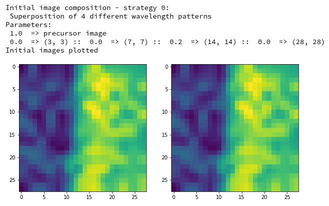
The enrichment of a large scale pattern by small scale fluctuations may support the creation of clearer OIP-images.

Creation of an OIP-image from the results of a precursor run

Method “_derive_OIP_for_Prec_Img()” executes the optimization loop for the creation of an OIP-image based on the input image offered. This method uses the the same instances of the GradienTape object and function “_iterate()” as the precursor run itself. It calls a method “_oip_strat_0_optimization_loop()” performing the calculations during the optimization. To plot the image evolution we have to provide a figure with 8 sub-plots.

Jupyter cell 7:

 
#from IPython.core.display import display, HTML
#display(HTML("<style>div.output_scroll { height:44em; }</style>"))


# Derive an  OIP from a PRECURSOR IMAGE for a selected map 
# *********************************************************

# figure A - 8 frames
# -----------
#sizing
fig_size = plt.rcParams["figure.figsize"]
fig_size[0] = 16
fig_size[1] = 8
fig_a = plt.figure(1)
axa_1 = fig_a.add_subplot(241)
axa_2 = fig_a.add_subplot(242)
axa_3 = fig_a.add_subplot(243)
axa_4 = fig_a.add_subplot(244)
axa_5 = fig_a.add_subplot(245)
axa_6 = fig_a.add_subplot(246)
axa_7 = fig_a.add_subplot(247)
axa_8 = fig_a.add_subplot(248)
li_axa = [axa_1, axa_2, axa_3, axa_4, axa_5, axa_6, axa_7, axa_8]

# figure B - 2 vertical frames for last image + contrats enhancemnet 
# -----------
#sizing
fig_size = plt.rcParams["figure.figsize"]
fig_size[0] = 3
fig_size[1] = 7
#fig_b = plt.figure(2, figsize=(5,11.2))
fig_b = plt.figure(2)
ax1_1 = fig_b.add_subplot(211)
ax1_2 = fig_b.add_subplot(212)


# Parameters of the OIP-image optimization 
# ~~~~~~~~~~~~~~~~~~~~~~~~~~~~~~~~~~~~~~~~~
n_epochs = 1200          # should be divisible by 5  
n_steps = 6             # number of intermediate reports 
epsilon = 0.01          # step size for gradient correction  
conv_criterion = 2.e-4  # criterion for a potential stop of optimization 


with tf.device("/GPU:0"):
    MyOIP._derive_OIP_for_Prec_Img( n_epochs = n_epochs, n_steps = n_steps, 
                        epsilon = epsilon , conv_criterion = conv_criterion, 
                        li_axa = li_axa, ax1_1 = ax1_1, ax1_2 = ax1_2, 
                        b_stop_with_convergence=False, 
                        b_show_intermediate_images=True 
                        )

Note: You can use the first two out-commented statements at the cell’s top to control the height of the output window of your Jupyter cells. Just remove the “#” comment signs.

The result contains intermediate information on the loss values and convergence. This helps to determine the minimum number of epochs for an optional second run.

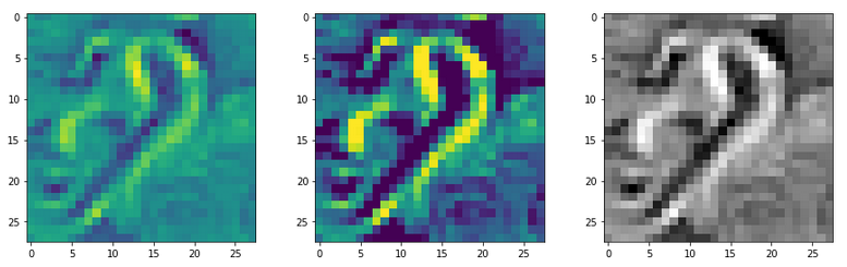
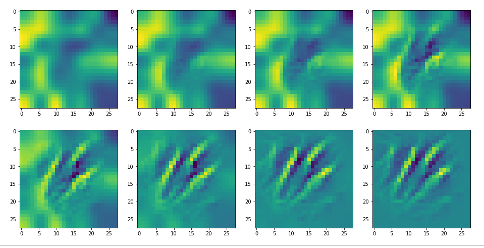
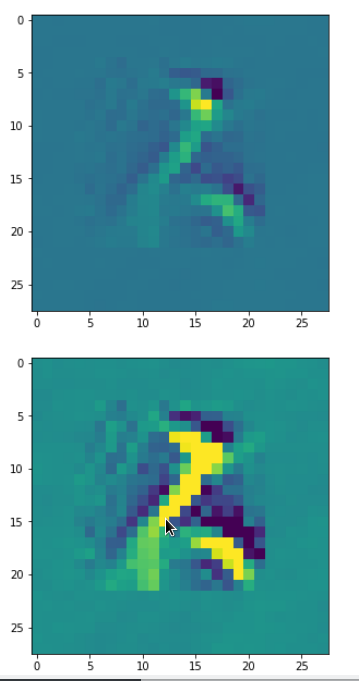
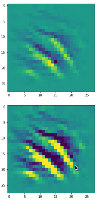
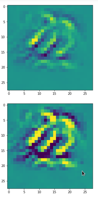
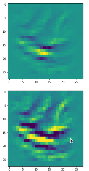
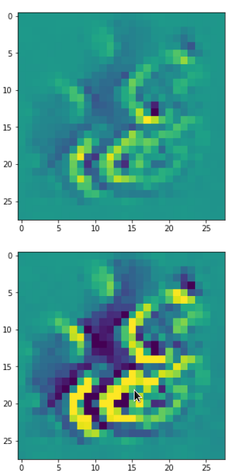
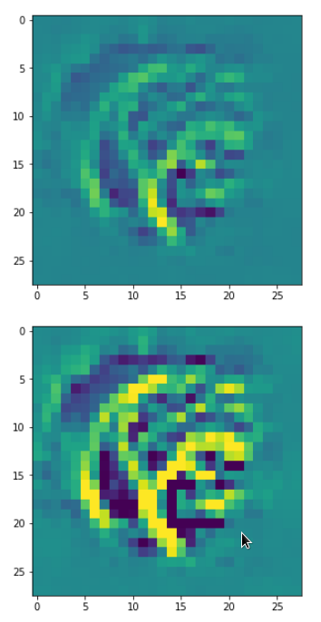
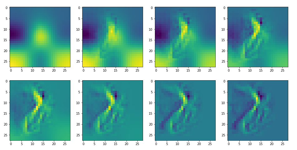
In the end we get a plot for the history of the image evolution out of the input patterns. The distance between the epochs for which the plots are done changes in a logarithmic manner. At the end our method calls “_transform_tensor_to_img()” with some standard parameters for a display of the OIP with contrast enhancement.

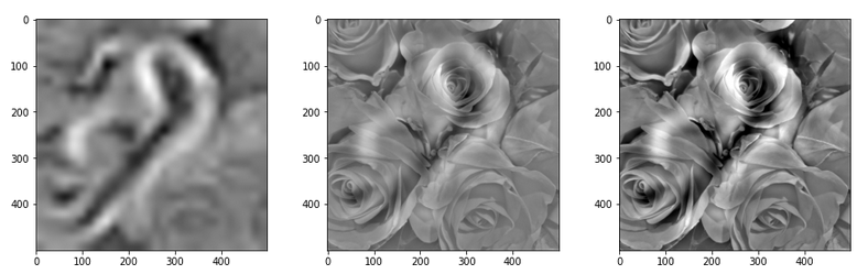
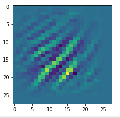
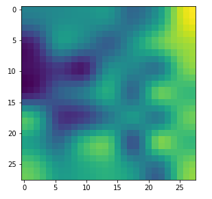
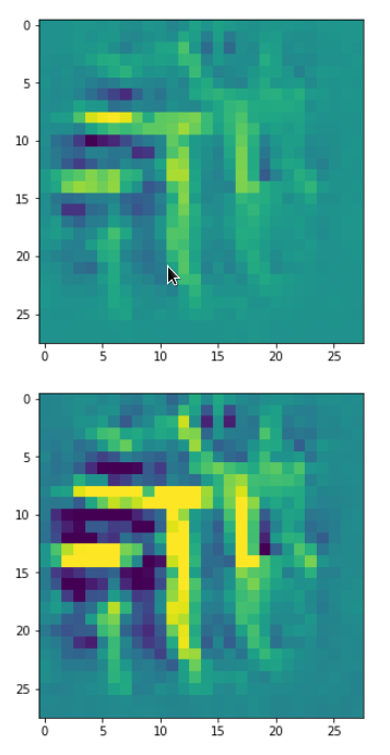
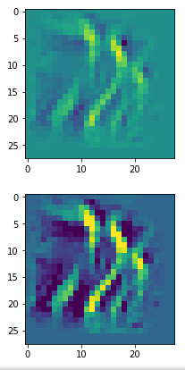
For the non-enriched large scale pattern displayed above we get:

*************
Start of optimization loop
*************
Strategy: Simple initial mixture of long and short range variations
Number of epochs =  1000
Epsilon =   0.01
*************
li_int =  [15, 30, 60, 120, 240, 480]
j:  0  :: loss_val =  0.9638658  :: loss_diff =  0.
9638658165931702

step 0 finalized
present loss_val =  0.9638658
loss_diff =  0.9638658165931702
Shape of intermediate img =  (28, 28)
j:  1  :: loss_val =  12.853093  :: loss_diff =  11.889227
j:  2  :: loss_val =  13.5863  :: loss_diff =  0.73320675
j:  3  :: loss_val =  14.277494  :: loss_diff =  0.69119453
j:  4  :: loss_val =  14.983041  :: loss_diff =  0.7055464
j:  5  :: loss_val =  15.694604  :: loss_diff =  0.7115631
j:  6  :: loss_val =  16.413284  :: loss_diff =  0.7186804
j:  7  :: loss_val =  17.148396  :: loss_diff =  0.73511124
...
...
j:  994  :: loss_val =  99.45101  :: loss_diff =  -0.003944397
j:  995  :: loss_val =  99.453865  :: loss_diff =  0.0028533936
j:  996  :: loss_val =  99.50871  :: loss_diff =  0.054847717
j:  997  :: loss_val =  99.47069  :: loss_diff =  -0.038024902
j:  998  :: loss_val =  99.51533  :: loss_diff =  0.044639587
j:  999  :: loss_val =  99.43279  :: loss_diff =  -0.08253479

step 999 finalized
present loss_val =  99.43279
loss_diff =  -0.08253479

Infos on pixel value distribution during contrast enhancement: 
max_orig =  4.7334514  :: avg_orig =  -1.2164214e-08  :: min_orig:  -3.6500213
std_dev_orig =  1.0
max_ay =  4.733451  :: avg_ay =  0.0  :: min_ay:  -3.6500208
std_dev_ay =  0.9999999
div =  3.562975788116455
max_fin =  1.6585106  :: avg_fin =  0.33000004  :: min_fin:  -0.69443035
std_dev_fin =  0.28066427

max_img =  255  :: avg_img =  85.10331632653062  :: min_img:  0
std_dev_img =  58.67217632503727

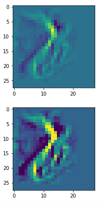
The last information lines reflect some data on the pixel value distribution during transformations for contrast enhancement. See the code of method “_transform_tensor_to_img()”.

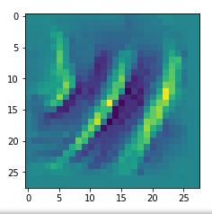
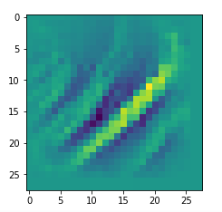
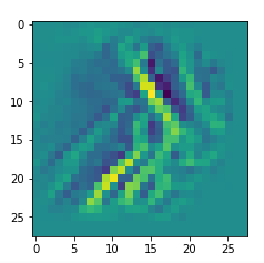
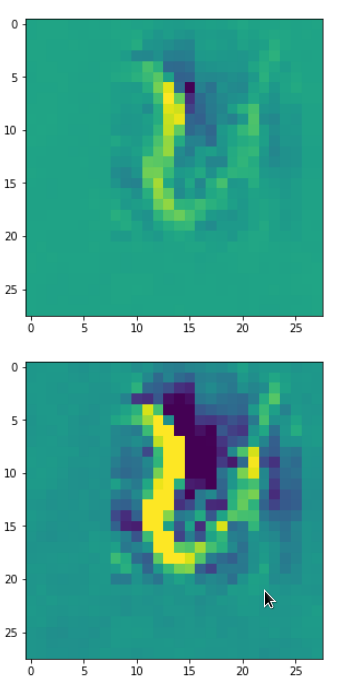
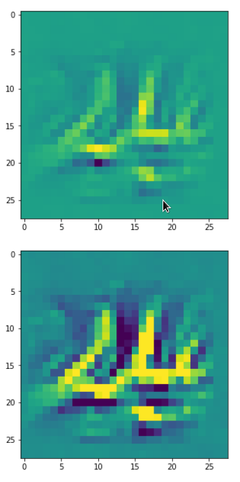
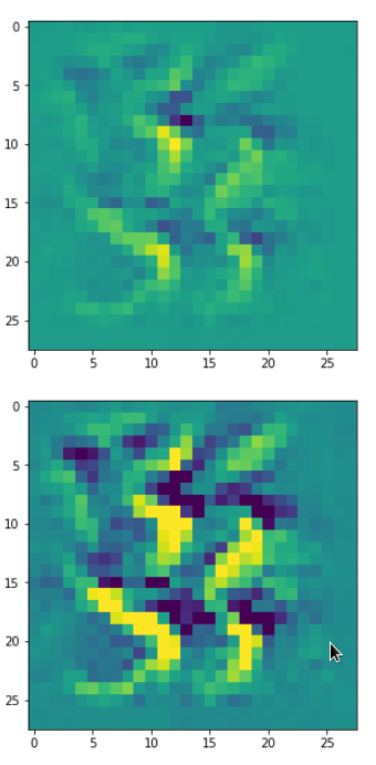
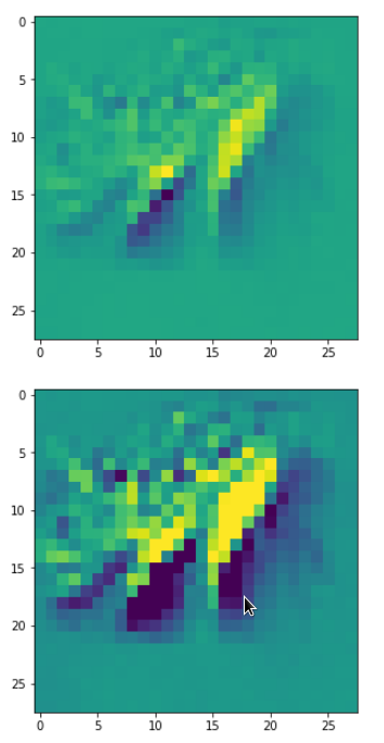
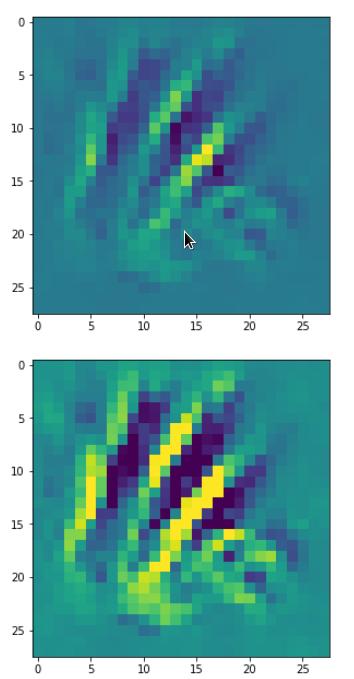
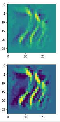
The resulting images are:

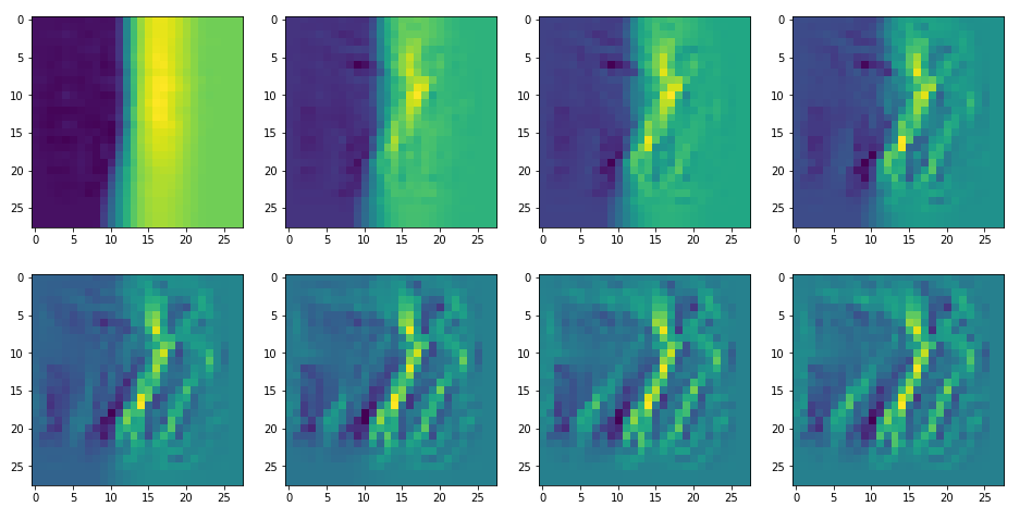
and

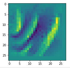
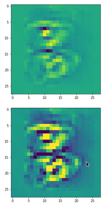
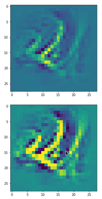
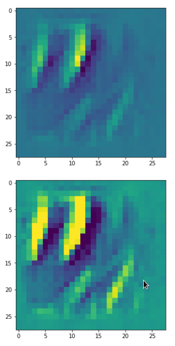
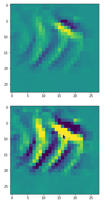
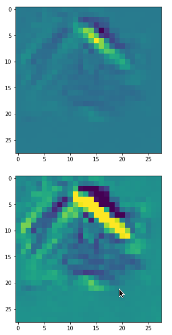
When you repeat the OIP-creation this for the enriched input image you get:

So, there are some differences – and, yes, you may want to play around a bit with the parameter options.

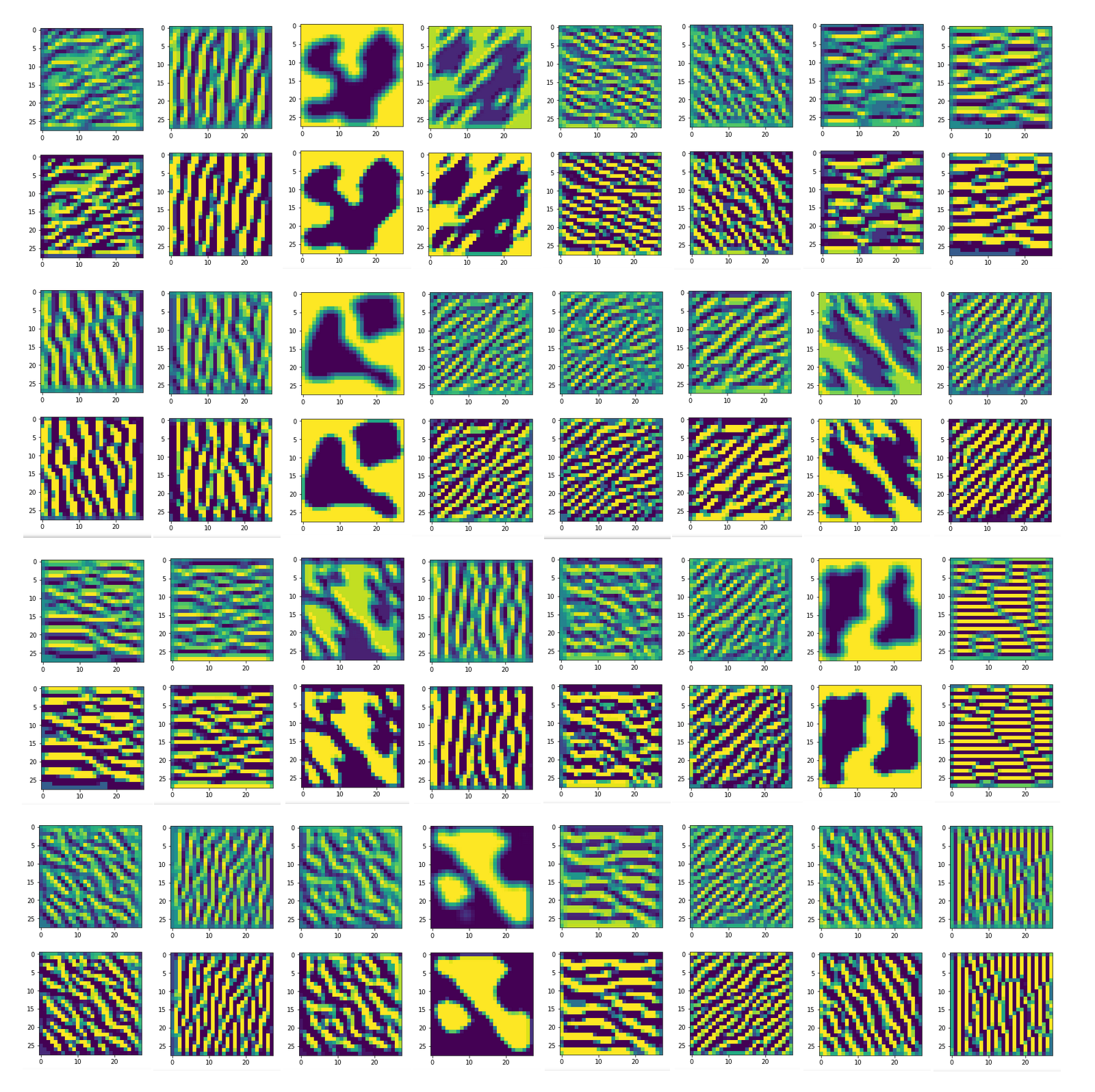
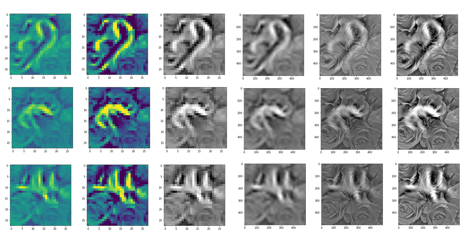
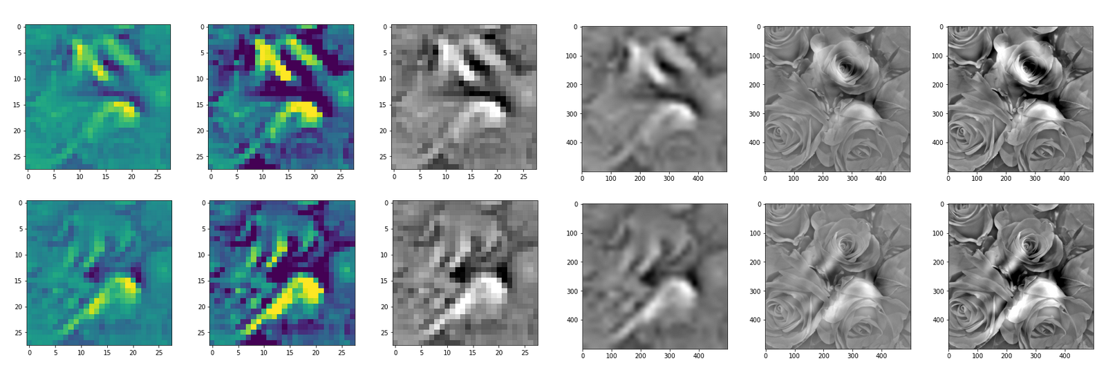
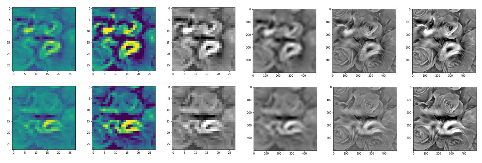
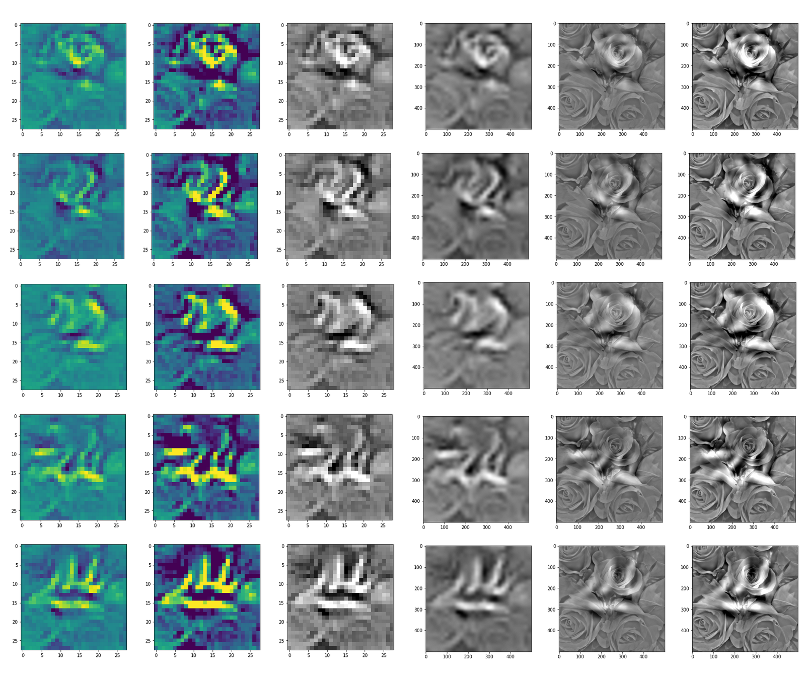
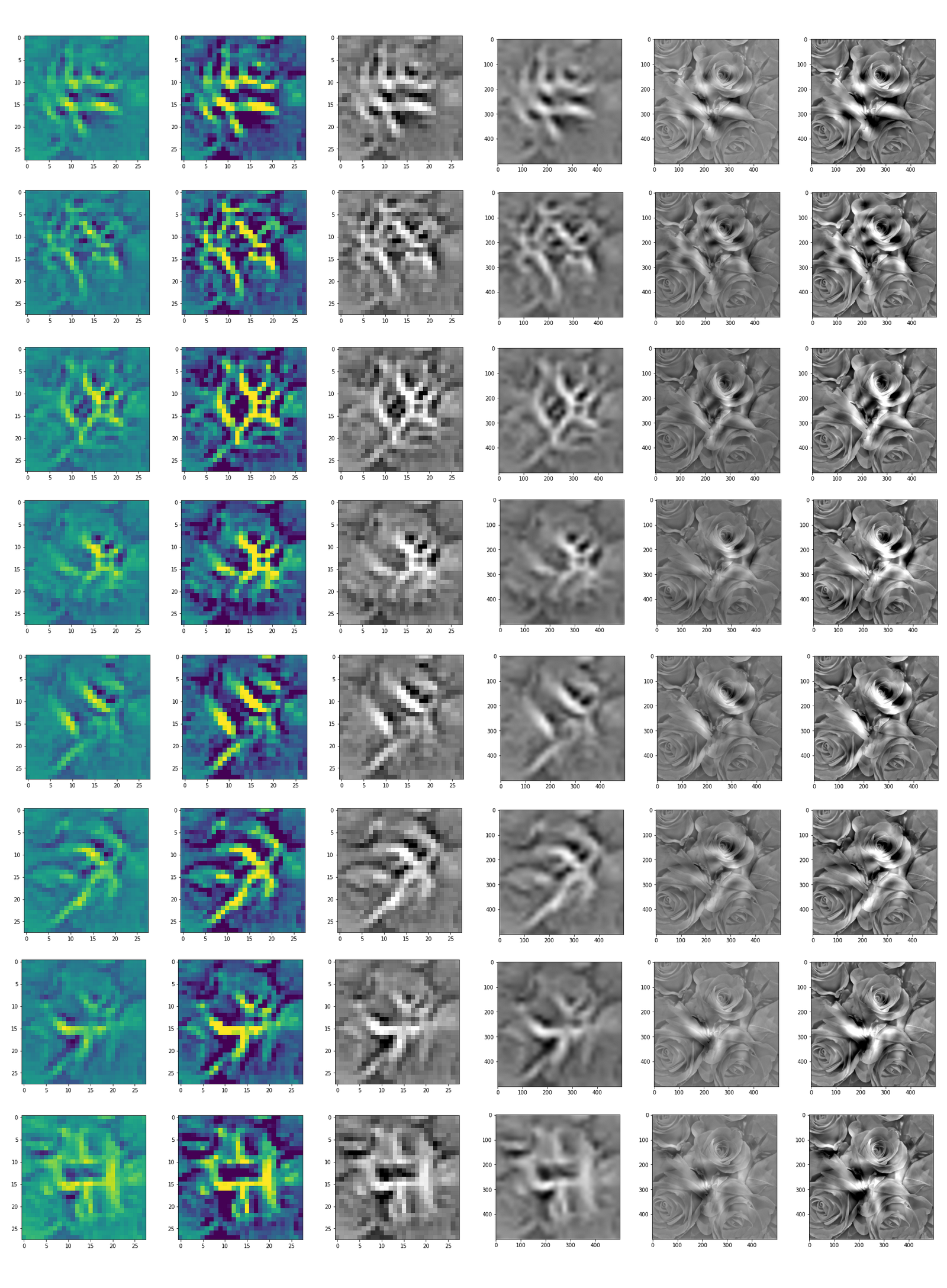
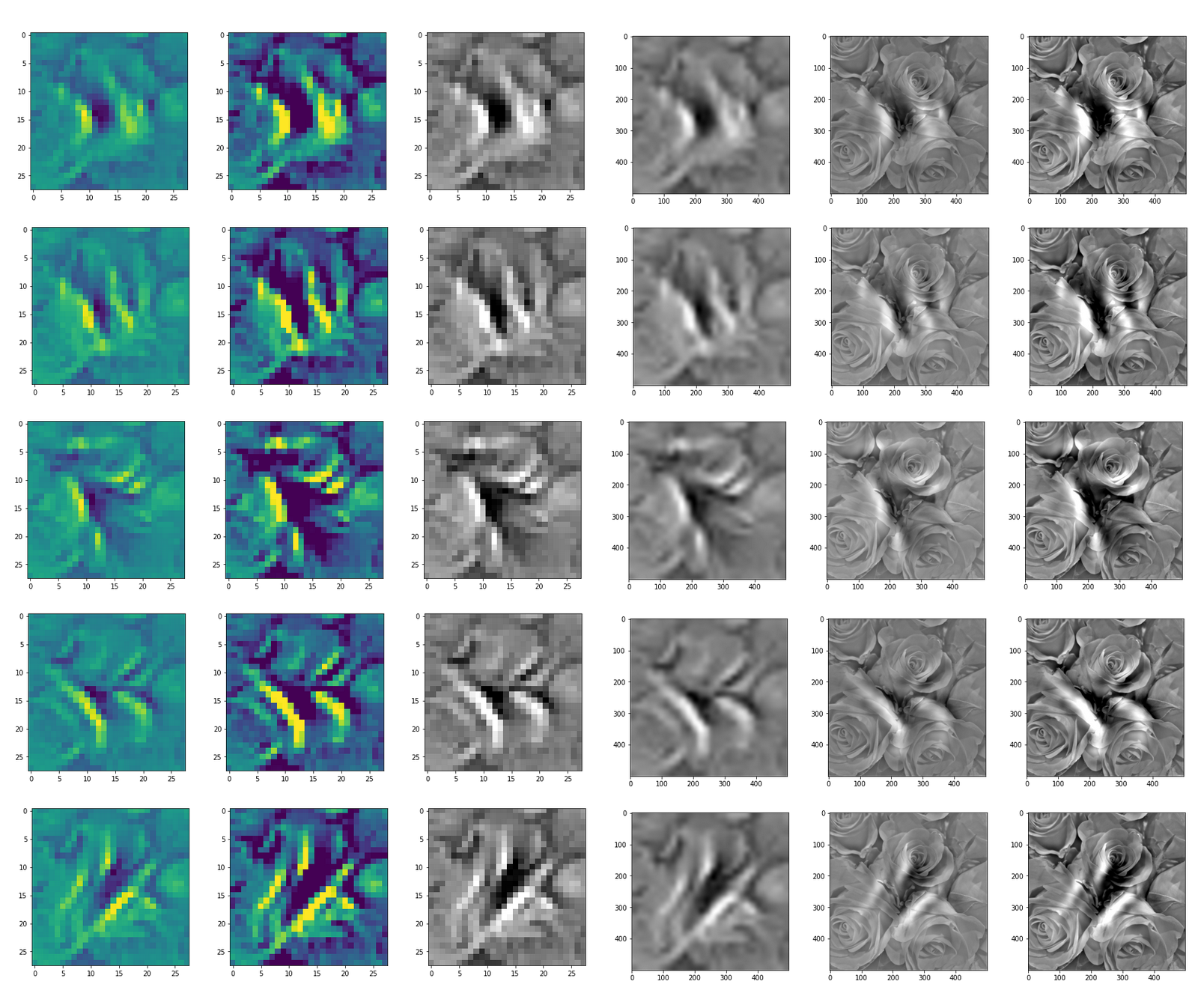
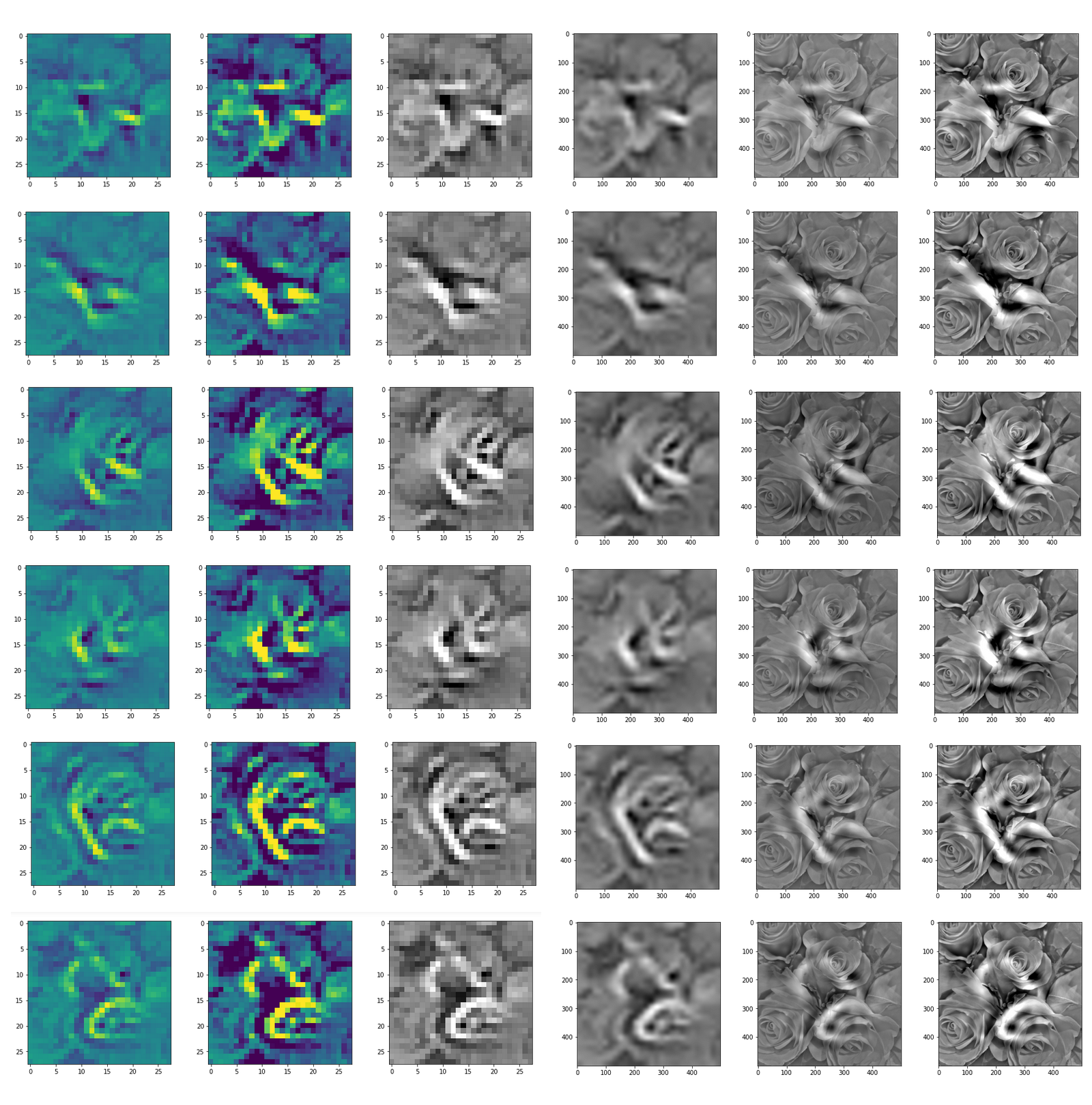
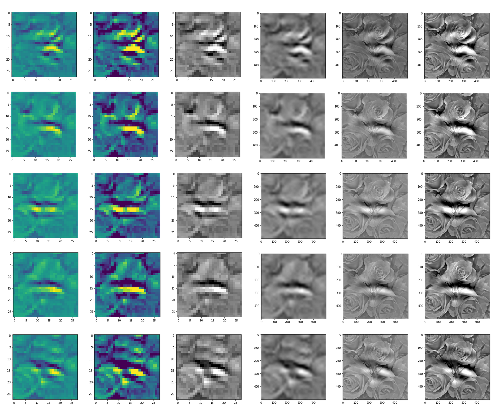
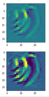
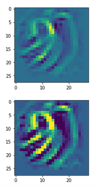
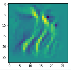
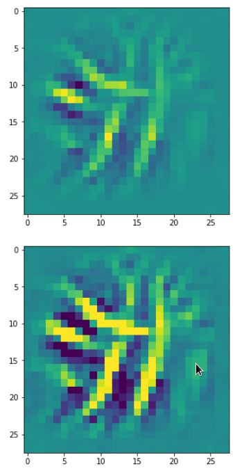
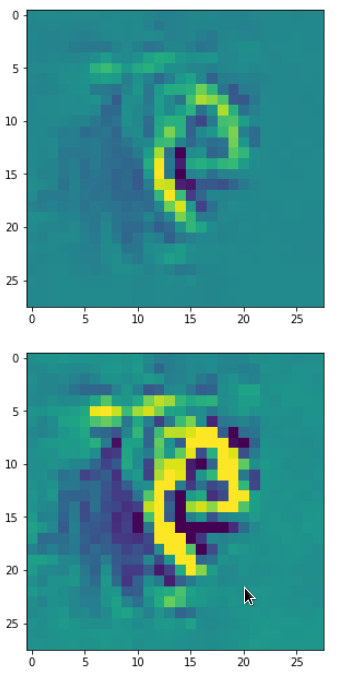
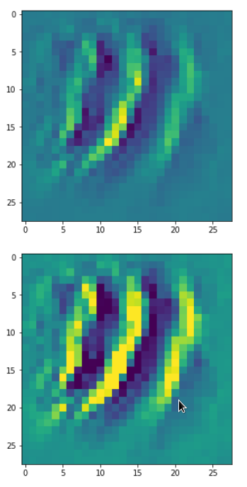
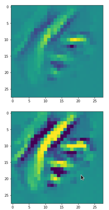
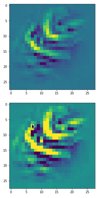
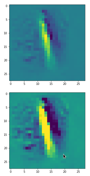
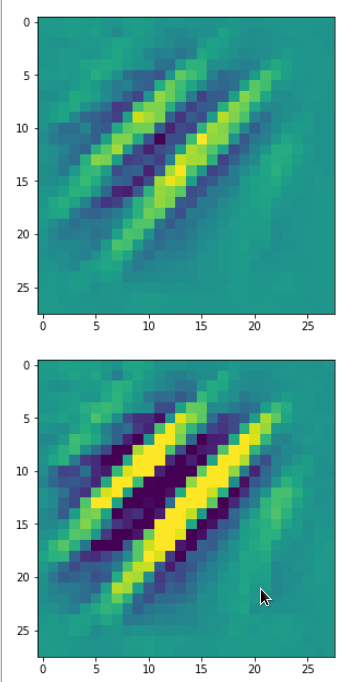
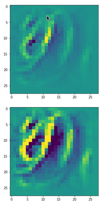
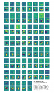
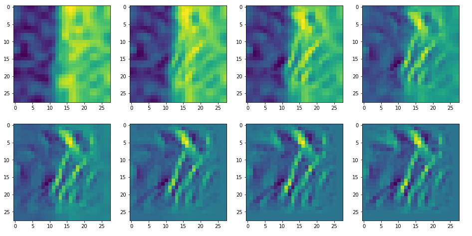
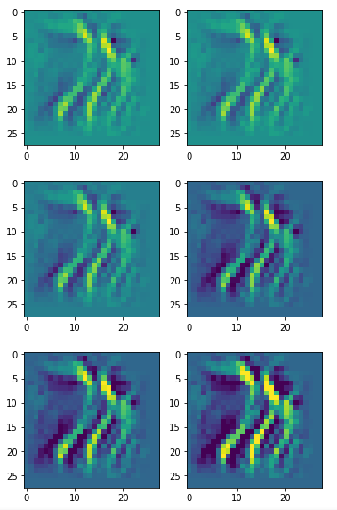
Below I present you the results for all eight long range patterns – un-enriched and for 1000 epochs.

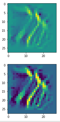
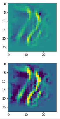
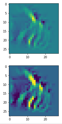
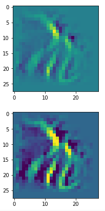
OIP-creation obviously depends to some extent on the input patterns offered. But there is an overall similarity.

Pick the OIP you like best. The loss values in order of the OIP-images are: 108.94, 105,95, 102.62, 96.02, 99.67, 100.75, 103.40, 99.45. (This shows by the way that the order in terms of a loss value after 10 tested epochs does not reflect the order after a full run over hundreds of epochs.)

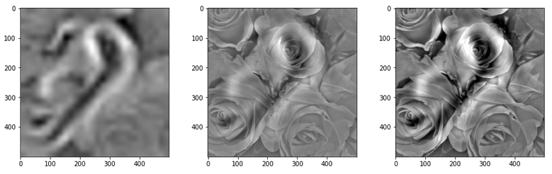
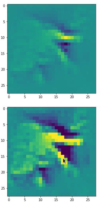
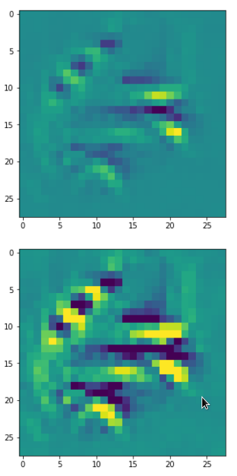
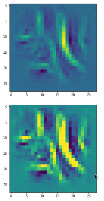
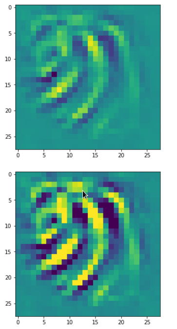
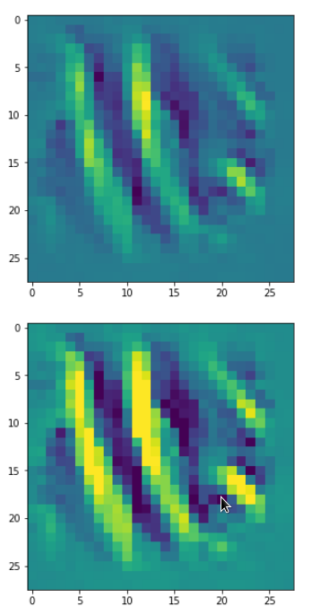
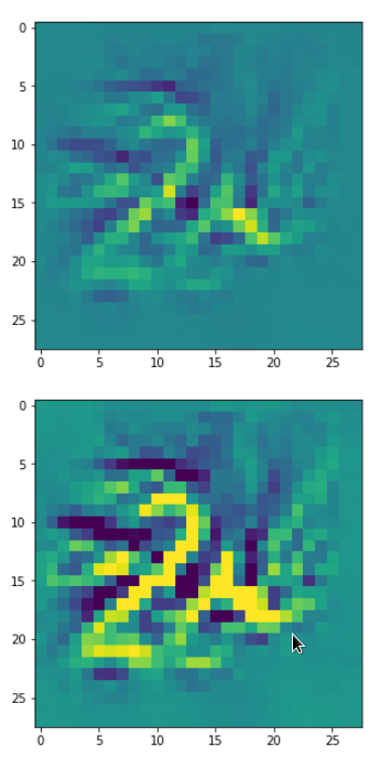
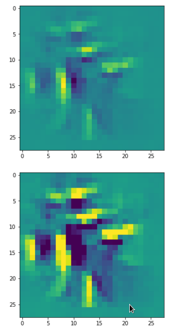
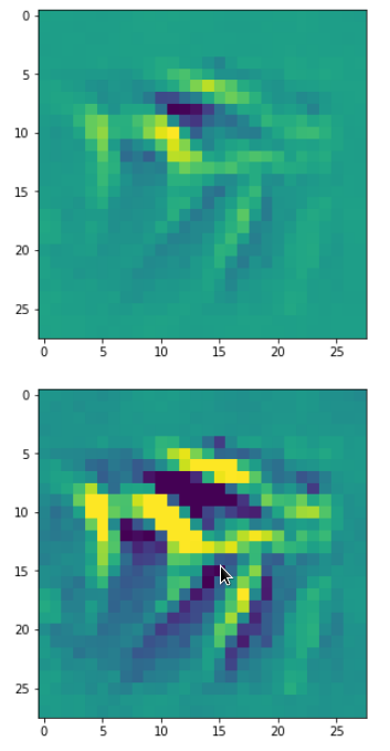
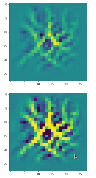
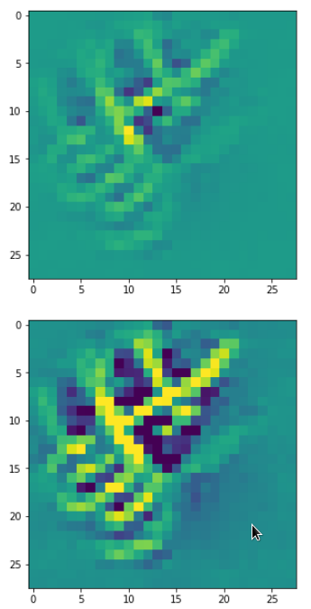
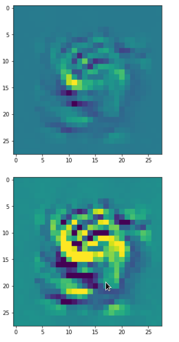
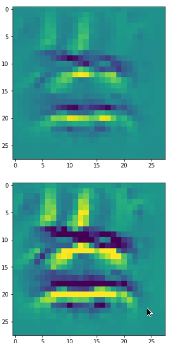
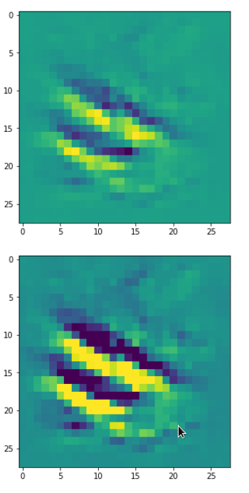
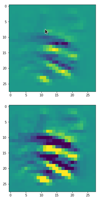
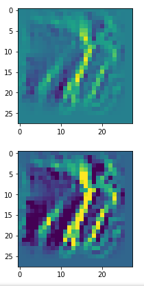
Play around with contrast enhancement

You may not be satisfied with the contrast enhancement and find it somewhat exaggerated. Can you change it? Yes, method “_transform_tensor_to_img()” provides two parameters for it. One (centre_move) is shifting the average of the values, the other (fact) the spread of the pixel values when mapping the calculated standardized values to the conventional range of [0, 255] for pixel values. Thecode reveals that some clipping is used, too.

The following Jupyter cell allows for a variation of the contrast related parameters for the present OIP-image whose original values are available from variable “_inp_img_data[0, :, :, 0]”.

Jupyter cell 8:

        
from IPython.core.display import display, HTML
display(HTML("<style>div.output_scroll { height:44em; }</style>"))

# figure B - 2 vertical frames for last image + contrats enhancemnet 
# -----------
#sizing
fig_size = plt.rcParams["figure.figsize"]
fig_size[0] = 6
fig_size[1] = 10
#fig_b = plt.figure(2, figsize=(5,11.2))
fig_b = plt.figure(1)
ax1_1 = fig_b.add_subplot(321)
ax1_2 = fig_b.add_subplot(322)
ax1_3 = fig_b.add_subplot(323)
ax1_4 = fig_b.add_subplot(324)
ax1_5 = fig_b.add_subplot(325)
ax1_6 = fig_b.add_subplot(326)
        
# -------------    
    
X_img = MyOIP._inp_img_data[0, :, :, 0]    

XN_img = X_img.numpy()
XT2_img = MyOIP._transform_tensor_to_img(X_img, centre_move = 0.5, fact = 2.0)

ax1_1.imshow(XN_img, cmap=plt.cm.get_cmap('viridis'))
ax1_2.imshow(XT2_img, cmap=plt.cm.get_cmap('viridis'))

XT3_img = MyOIP._transform_tensor_to_img(X_img, centre_move = 0.42, fact = 1.8)
XT4_img = MyOIP._transform_tensor_to_img(X_img, centre_move = 0.33, fact = 1.4)

ax1_3.imshow(XT3_img, cmap=plt.cm.get_cmap('viridis'))
ax1_4.imshow(XT4_img, 
cmap=plt.cm.get_cmap('viridis'))

XT5_img = MyOIP._transform_tensor_to_img(X_img, centre_move = 0.33, fact = 1.2)
XT6_img = MyOIP._transform_tensor_to_img(X_img, centre_move = 0.33, fact = 0.9)

ax1_5.imshow(XT5_img, cmap=plt.cm.get_cmap('viridis'))
ax1_6.imshow(XT6_img, cmap=plt.cm.get_cmap('viridis'))

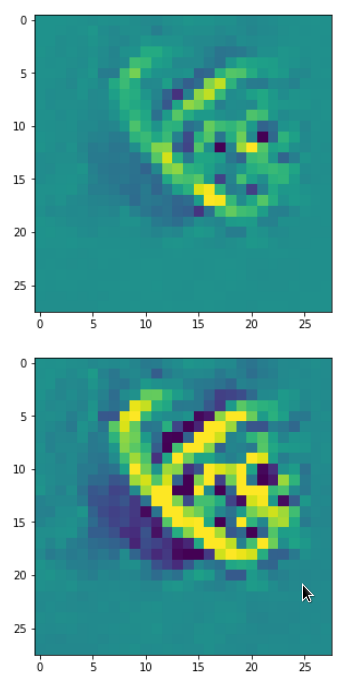
The images look like:

Enough options to create nice OIP-images.

If you do not care about a precursor run in the first place ….

Now, a precursor-run may be too costly for you. You just want to play around with some statistical input image and a map in a trial and error fashion. Then you may just use the following two Jupyter cells:

Jupyter cell 9:

        
from IPython.core.display import display, HTML
display(HTML("<style>div.output_scroll { height:34em; }</style>"))

# build simple initial image composed of fluctuations  
# *******************************************************

# figure
# -----------
#sizing
fig_size = plt.rcParams["figure.figsize"]
fig_size[0] = 10
fig_size[1] = 5
fig1 = plt.figure(1)
ax1_1 = fig1.add_subplot(121)
ax1_2 = fig1.add_subplot(122)

# OIP function to setup an initial image 
initial_img = MyOIP._build_initial_img_data(  strategy = 0, 
                                 li_epochs    = (20, 50, 100, 400), 
                                 li_facts     = (0.2, 0.0, 0.0, 0.0),
                                 li_dim_steps = ( (3,3), (7,7), (14,14), (28,28) ), 
                                 b_smoothing = False,
                                 ax1_1 = ax1_1, ax1_2 = ax1_2)

with output

Then use

Jupyter cell 10:

   
# Derive a single OIP from an input image with statistical fluctuations of the pixel values 
# ******************************************************************

# figure A - 8 frames
# -----------
#sizing
fig_size = plt.rcParams["figure.figsize"]
fig_size[0] = 16
fig_size[1] = 8
fig_a = plt.figure(1)
axa_1 = fig_a.add_subplot(241)
axa_2 = fig_a.add_subplot(242)
axa_3 = fig_a.add_subplot(243)
axa_4 = fig_a.add_subplot(244)
axa_5 = fig_a.add_subplot(245)
axa_6 = fig_a.add_subplot(246)
axa_7 = fig_a.add_subplot(247)
axa_8 = fig_a.add_subplot(248)
li_axa = [axa_1, axa_2, axa_3, axa_4, axa_5, axa_6, axa_7, axa_8]

# figure B - 2 vertical frames for last image + contrats enhancemnet 
# -----------
#sizing
fig_size = plt.rcParams["figure.figsize"]
fig_size[0] = 3
fig_size[1] = 7
#fig_b = plt.figure(2, figsize=(5,11.2))
fig_b = plt.figure(2)
ax1_1 = fig_b.add_subplot(211)
ax1_2 = fig_b.add_subplot(212)


map_index = 38          # map-index we are interested in 
n_epochs = 1000           # should be divisible by 5  
n_steps = 6             # number of intermediate reports 
epsilon = 0.01          # step size for gradient correction  
conv_criterion = 2.e-4  # criterion for a potential stop of optimization 

MyOIP._derive_OIP(map_index = map_index, 
           
       n_epochs = n_epochs, n_steps = n_steps, 
                  epsilon = epsilon , conv_criterion = conv_criterion, 
                  b_stop_with_convergence=False,
                 li_axa = li_axa,
                 ax1_1 = ax1_1, ax1_2 = ax1_2)

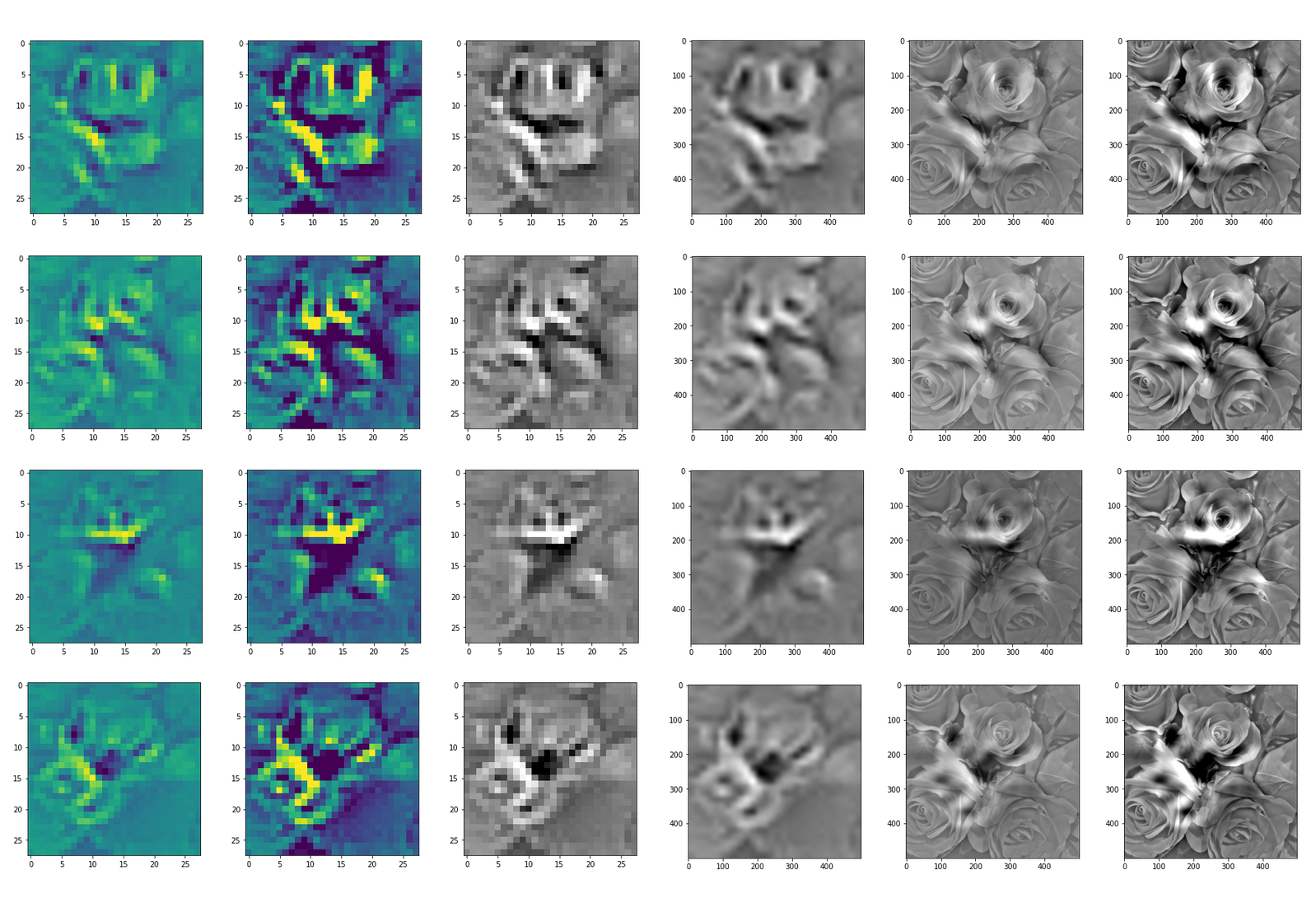
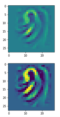
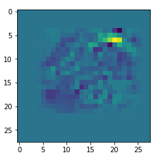
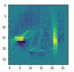
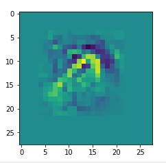
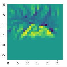
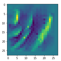
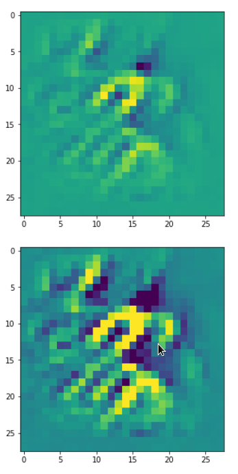
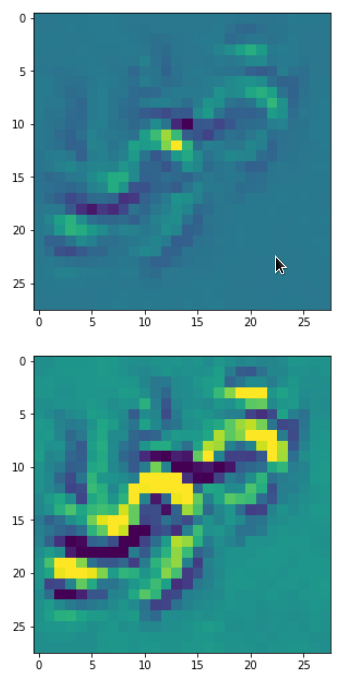
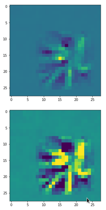
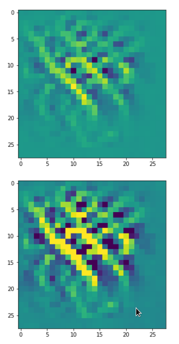
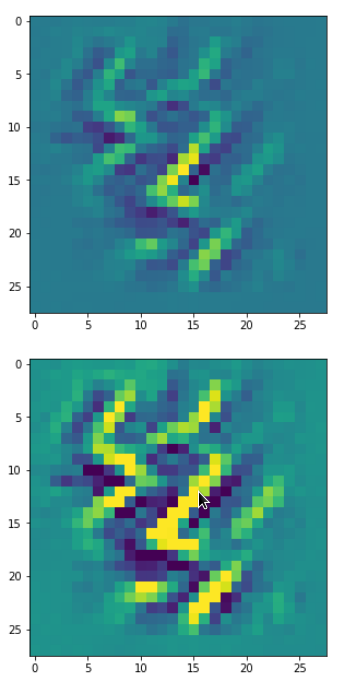
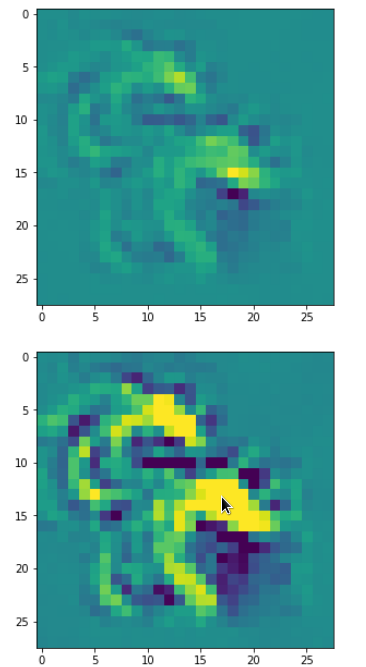
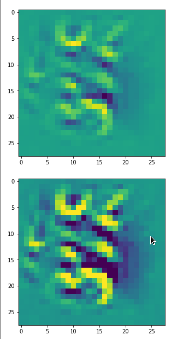
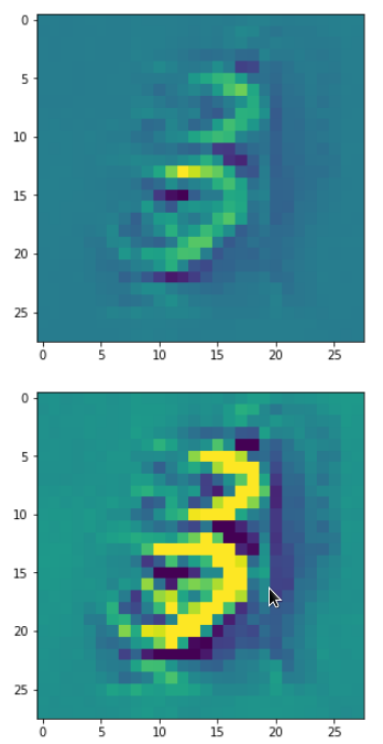
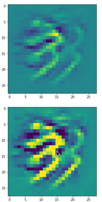
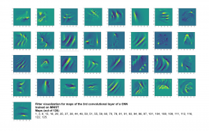
It produces an image output:

The comparison with other OIP-images above again shows a significant dependency of the outcome of our algorithm on the input image offered. Especially, when large scale OIPs are relevant for a map. The trial-and-error approach often does not reveal the repetitions of some basic pattern at different positions in the OIP-image as clearly as a systematic test of patterns does.

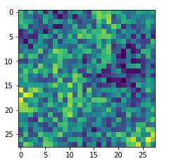
By the way: T was lucky in the above case that I got a reasonable OIP at all! Actually, I needed around 10 trials to get it. But if you tried e.g. with dominant small scale fluctuations defined by

initial_img = MyOIP._build_initial_img_data(  strategy = 0, 
                                 li_epochs    = (20, 50, 100, 400), 
                                 li_facts     = (0.1, 0.0, 0.0, 0.2),
                                 li_dim_steps = ( (3,3), (7,7), (14,14), (28,28) ), 
                                 b_smoothing = False,
                                 ax1_1 = ax1_1, ax1_2 = ax1_2)

then the random number functionality will produce an input image as

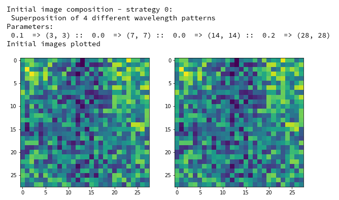
which in turn will consistently lead to zero results

Start of optimization loop
*************
Strategy: Simple initial mixture of long and short range variations
Number of epochs =  1000
Epsilon =   0.01
*************
li_int =  [15, 30, 60, 120, 240, 480]
j:  0  :: loss_val =  0.0  :: loss_diff =  0.0
0-values, j=  0  loss =  0.0  avg_loss =  0.0

step 0 finalized
present loss_val =  0.0
loss_diff =  0.0
j:  1  :: loss_val =  0.0  :: loss_diff =  0.0
0-values, j=  1  loss =  0.0  avg_loss =  0.0
j:  2  :: loss_val =  0.0  :: loss_diff =  0.0
...
...
0-values, j=  10  loss =  0.0  avg_loss =  0.0
More than 10 times zero values - Try a different initial random distribution of pixel values

for map 38. Map 38 does not “like” random small scale fluctuations; it sees no pattern in them which would pass its underlying filter combination. Well, this was actually the main reason for a more systematic approach based on large scale patterns … .

But even in a trial-and-error approach you should always test pure long scale fluctuations first.

Does the code run as fast with TF 2.3.1?

No, it does not. Actually, it runs by a factor of 4 to 5 slower! The graphics card is used much less. I could not pin down the reason yet but I think that there is some inefficiency in data transfers between the graka’s environment and the CPU’s environment in the newer version of Tensorflow – maybe there are even unnecessary transfers occurring. If the problems with TF 2.3 do not disappear in a later version, I will file a bug report.

Code extension to cover multiple maps in one run?

Studying the code a bit will enable you to modify, beautify and extend it. Personally, I just have no time which I could invest in major changes right now. If you want to extend the program yourself to cover multiple maps in one run I recommend the following approach:

Build loops across the methods “_prepare_precursor()” and “_precursor()” for a range of defined maps. Save at least some of the identified basic fluctuation pattern for initial input images. Then build and start a method for a separate run which reconstructs input images from the saved fluctuation patterns and builds the related OIP-images – a process which does not take much time. Select theone with highest loss for each map. Then you should add a method for the display of the remaining OIP-images on an image grid for all maps- this would be similar to what we did with activation patterns in previous articles.

Conclusion

The visualization of filters, i.e. the creation of input images with patterns that trigger a map optimally, can become a hard business when we work with maps of deep convolutional layers. Some maps there may not react to input images with purely statistical pixel values and no dominant fluctuation pattern on longer length scales. During this article I have discussed the methods of a simple Python class which allows at least for a more systematic, though GPU/CPU-intensive, approach. It should be easy for readers who work a bit with Python to extend the code and tackle more elaborate tasks – also outside the MNIST case.

In the next article of this series

A simple CNN for the MNIST dataset – XII – filter visualization for maps of the first two convolutional layers

we shall look a bit at the other convolutional layers. So far we have only covered of the deepest Conv layer. Later on we shall close our first encounter with a (simple) CNN by answering a question posed at the series’ beginning: What changes if we re-train the CNN on a shuffled MNIST data set?

Some Python code for OIP detection and creation

 
'''
Module to create OIPs as visualizations of filters of a simple CNN for the MNIST data set
@version: 0.6, 10.10.2020
@change: V0.5:  was based on version 0.4 which was originally created in Jupyter cells
@change: V0.6: General revision of class "my_OIP" and its methods
@change: V0.6: Changes to the documentation 
@attention: General status: For experimental purposes only! 
@requires: A full CNN trained on MNIST data 
@requires: A Keras model of the CNN and weight data saved in a h5-file, e.g."cnn_MIST_best.h5". 
           This file must be placed in the main directory of the Jupyter notebooks.
@requires: A Jupyter environment - from where the class My_OIP is called and where plotting takes place 
@note: The description to the interface to the class via the __init__()-method may be incomplete
@note: The use of prefixes li_ and ay_ is not yet consistent. ay_ should indicate numpy arrays, li_ instead normal Python lists
@warning: This version has not been tested outside a Jupyter environment - plotting in GTK/Qt-environment may require substantial changes 
@status: Under major development with frequent changes 
@author: Dr. Ralph Mönchmeyer
@copyright: Simplified BSD License, 10.10.2020. Copyright (c) 2020, Dr. Ralph Moenchmeyer, Augsburg, Germnay

Redistribution and use in source and binary forms, with or without
modification, are permitted provided that the following conditions are met:

1. Redistributions of source code must retain the above copyright notice, this
   list of conditions and the following disclaimer.
2. Redistributions in 
binary form must reproduce the above copyright notice,
   this list of conditions and the following disclaimer in the documentation
   and/or other materials provided with the distribution.

THIS SOFTWARE IS PROVIDED BY THE COPYRIGHT HOLDERS AND CONTRIBUTORS "AS IS" AND
ANY EXPRESS OR IMPLIED WARRANTIES, INCLUDING, BUT NOT LIMITED TO, THE IMPLIED
WARRANTIES OF MERCHANTABILITY AND FITNESS FOR A PARTICULAR PURPOSE ARE
DISCLAIMED. IN NO EVENT SHALL THE COPYRIGHT OWNER OR CONTRIBUTORS BE LIABLE FOR
ANY DIRECT, INDIRECT, INCIDENTAL, SPECIAL, EXEMPLARY, OR CONSEQUENTIAL DAMAGES
(INCLUDING, BUT NOT LIMITED TO, PROCUREMENT OF SUBSTITUTE GOODS OR SERVICES;
LOSS OF USE, DATA, OR PROFITS; OR BUSINESS INTERRUPTION) HOWEVER CAUSED AND
ON ANY THEORY OF LIABILITY, WHETHER IN CONTRACT, STRICT LIABILITY, OR TORT
(INCLUDING NEGLIGENCE OR OTHERWISE) ARISING IN ANY WAY OUT OF THE USE OF THIS
SOFTWARE, EVEN IF ADVISED OF THE POSSIBILITY OF SUCH DAMAGE.
'''

# Modules to be imported - these libs must be imported in a Jupyter cell nevertheless 
# ~~~~~~~~~~~~~~~~~~~~~~~~
import time 
import sys 
import math
import os 
from os import path as path

import numpy as np
from numpy import save  # used to export intermediate data
from numpy import load

import scipy
from sklearn.preprocessing import StandardScaler
from itertools import product 

import tensorflow as tf
from tensorflow import keras as K
from tensorflow.python.keras import backend as B  # this is the only version compatible with TF 1 compat statements
#from tensorflow.keras import backend as B 
from tensorflow.keras import models
from tensorflow.keras import layers
from tensorflow.keras import regularizers
from tensorflow.keras import optimizers
from tensorflow.keras.optimizers import schedules
from tensorflow.keras.utils import to_categorical
from tensorflow.keras.datasets import mnist

from tensorflow.python.client import device_lib

import matplotlib as mpl
from matplotlib import pyplot as plt
from matplotlib.colors import ListedColormap
import matplotlib.patches as mpat 

from IPython.core.tests.simpleerr import sysexit

class My_OIP:
    '''
    @summary: This class allows for the creation and the display of OIP-patterns, 
              to which a selected map of a CNN-model and related filters react maximally
    
    @version: Version 0.6, 10.10.2020
    ~~~~~~~~~~~~~~~~~~~~~~~~~~~~~~~~~~
    @change: Revised methods 
    @requires: In the present version the class My_OIP requires: 
                * a CNN-model which works with standardized (!) input images, size 28x28,
                * a CNN-Modell which was trained on MNIST digit data,
                * exactly 4 length scales for random data fluctations are used to compose initial statistial image data 
                  (the length scales should roughly have a factor of 2 between them) 
                * Assumption : exactly 1 input image and not a batch of images is assumed in various methods 
    
    @note: Main Functions:     
    0) _init__()
    1) _load_cnn_model()             => load cnn-model
    2) _build_oip_model()            => build an oip-model to create OIP-images
    3) _setup_gradient_tape_and_iterate_function()        
                                    => Implements TF2 GradientTape to watch input data for eager gradient calculation
                                    => Creates a convenience function by the help of Keras to iterate and optimize the OIP-adjustments
    4) _oip_strat_0_optimization_loop():
                                     => Method implementing a simple strategy to create OIP-images, 
                                        based on superposition of random data on long range data (compared to 28 px) 
                                        The optimization uses "gradient ascent" to get an optimum output of the selected Conv map 

    6) _derive_OIP():                => Method used to start the creation of an OIP-image for a chosen map 
                                        - based on an input image with statistical random date 
    6) _derive_OIP_for_Prec_Img():   => Method used to start the creation of an OIP-image for a chosen map 
                                       - based on an input image with was derived from a PRECURSOR run, 
                                       which tests the reaction of the map to large scale fluctuations 
                                        
    7) _build_initial_img_data():    => Builds an input image based on random data for fluctuations on 4 length scales 
    8) _build_initial_img_from_prec():    
                                     => Reconstruct an input image based on saved random data for long range fluctuations 
    9) _prepare_precursor():         => Prepare a _precursor run by setting up TF2 GradientTape and the _iterate()-function 
    10) _precursor():                => Precursor run which systematically tests the reaction of a selected convolutional map 
                                        to long range fluctuations based on a (3x3)-grid upscaled to the real image size  
    11) _display_precursor_imgs():   => A method which plots up to 8 selected precursor images with fluctuations,
                                        which triggered a maximum map reaction 
    12) _transfrom_tensor_to_img():  => A method which allows to transform tensor data of a standardized (!) image to standard image data 
                                        with (gray)pixel valus in [0, 255]. Parameters allow for a contrast enhancement. 
    
    Usage hints 
    ~~~~~~~~~~~
    @note: If maps of a new convolutional layer are to be investigated then method _build_oip_model(layer_name) has to be rerun 
           with the layer's name as input parameter
    '''
    
    # Method to initialize an instantiation object 
    # ~~~~~~~~~~~~~~~~~~~~~~~~~~~~~~~~~~~~~~~~~~~~~
    def __init__(self, cnn_model_file = 'cnn_MNIST_best.h5', 
                 layer_name = 'Conv2D_3', 
                 map_index = 0, 
                 img_dim = 28, 
                 b_build_oip_model = True  
                ): 
        '''
        @summary: Initialization of an object instance - read in a CNN model, build an OIP-Model 
        @note: Input: 
        ~~~~~~~~~~~~
        @param cnn_model_file:  Name of a file containing a fully trained CNN-model; 
                                the model can later be overwritten by self._load_cnn_model()
        @param layer_name:      We can define a layer name, which we are interested in,  already when starting;
                                the layer can later be overwritten by self._build_oip_model()
        @param map_index:       We can define a map, which we are interested in,  already when starting;
                                A map-index is NOT required for building the OIP-model, but for the GradientTape-object 
        @param img_dim:         The dimension of the assumed quadratic images (2 for MNIST)

        @note: Major internal variables:
        ~~~~~~~~~~~~~~~~~~~~~~~~~~~~~~~
        @ivar _cnn_model:        A reference to the CNN model object
        @ivar _layer_name:       The name of convolutional layer 
                                 (can be overwritten by method _build_oip_model() ) 
        @ivar _map_index:        Index of the map in the chosen layer's output array 
                                 (can later be overwritten by other methods) 
        @ivar _r_cnn_inputs:     A reference to the input tensor of the CNN model 
                                 Could be a batch of images; but in this class only 1 image is assumed
        @ivar _layer_output:     Tensor with all maps of a certain layer    
        @ivar _oip_submodel:     A new model connecting the 
input of the CNN-model with a certain map's (!) output
        @ivar _tape:             An instance of TF2's GradientTape-object 
                                    Watches input, output, loss of a model 
                                    and calculates gradients in TF2 eager mode 
        @ivar _r_oip_outputs:    Reference to the output of the new OIP-model = map-activation
        @ivar _r_oip_grads:      Reference to gradient tensors for the new OIP-model (output dependency on input image pixels)
        @ivar _r_oip_loss:       Reference to a loss defined on the OIP-output - i.e. on the activation values of the map's nodes;
                                 Normally chosen to be an average of the nodes' activations 
                                 The loss defines a hyperplane on the (28x28)-dim representation space of the input image pixel values  
        @ivar _val_oip_loss:     Loss value for a certain input image 
        @ivar _iterate           Reference toa Keras backend function which invokes the new OIP-model for a given image
                                 and calculates both loss and gradient values (in TF2 eager mode) 
                                 This is the function to be used in the optimization loop for OIPs
        
        @note: Internal Parameters controlling the optimization loop:
        ~~~~~~~~~~~~~~~~~~~~~~~~~~~~~~~~~~~~~~~~~~~
        @ivar _oip_strategy:        0, 1 - There are two strategies to evolve OIP patterns out of statistical data 
                                    - only the first strategy is supported in this version 
                                    Both strategies can be combined with a precursor calculation 
                                    0: Simple superposition of fluctuations at different length scales
                                    1: NOT YET SUPPORTED 
                                    Evolution over partially evolved images based on longer scale variations 
                                    enriched with fluctuations on shorter length scales 

        @ivar _ay_epochs:           A list of 4 optimization epochs to be used whilst 
                                    evolving the img data via strategy 1 and intermediate images 
        @ivar _n_epochs:            Number of optimization epochs to be used with strategy 0 
        @ivar _n_steps:             Defines at how many intermediate points we show images and report 
                                    during the optimization process 
        @ivar _epsilon:             Factor to control the amount of correction imposed by the gradient values of the oip-model 

        @note: Input image data of the OIP-model and references to it 
        ~~~~~~~~~~~~~~~~~~~~~~~~~~~~~~~~~~
        @ivar _initial_precursor_img:  The initial image to start a precursor optimization with.
                                       Would normally be an image of only long range fluctuations. 
        @ivar _precursor_image:        The evolved image created and selected by the precursor loop 

        @ivar _initial_inp_img_data:  A tensor representing the data of the input image 
        @ivar _inp_img_data:          A tensor representig the 
        @ivar _img_dim:               We assume quadratic images to work with 
                                      with dimension _img_dim along each axis
                                      For the time being we only support MNIST images 
        
        @note: Internal parameters controlling the composition of random initial image data 
        ~~~~~~~~~~~~~~~~~~~~~~~~~~~~~~~~~~~~~~~~~~~
        @ivar _li_dim_steps:        A list of the intermediate dimensions for random data;
                                    these data are smoothly scaled to the image dimensions 
        @ivar _ay_facts:            A Numpy array of 4 factors to control the amount of 
                                    contribution of the statistical 
variations 
                                    on the 4 length scales to the initial image
        
        @note: Internal variables to save data of a precursor run
        ~~~~~~~~~~~~~~~~~~~~~~~~~~~~~~~~~~~~~~~~~~~~~~~~~~~~~~~~ 
        @ivar _list_of_covs: list of long range fluctuation data for a (3x3)-grid covering the image area 
        @ivar _li_fluct_enrichments: [li_facts, li_dim_steps] data for enrichment with small fluctuations 
        
        
        @note: Internal variables for plotting
        ~~~~~~~~~~~~~~~~~~~~~~~~~~~~~~~~~~~~~~~~~~~
        @ivar _li_axa: A Python list of references to external (Jupyter-) axes-frames for plotting 
        
        '''    
        
        # Input data and variable initializations
        # ****************************************
        
        # the model 
        # ~~~~~~~~~~
        self._cnn_model_file = cnn_model_file
        self._cnn_model      = None 
        
        # the chosen layer of te CNN-model
        self._layer_name = layer_name
        # the index of the map in the layer array
        self._map_index  = map_index
        
        # References to objects and the OIP-submodel
        # ~~~~~~~~~~~~~~~~~~~~~~~~~~~~~~
        self._r_cnn_inputs  = None # reference to input of the CNN_model, also used in the oip-model  
        self._layer_output  = None
        self._oip_submodel  = None
        
        # References to watched GradientTape objects 
        # ~~~~~~~~~~~~~~~~~~~~~~~~~~~~~~
        self._tape          = None # TF2 GradientTape variable
        # some "references"
        self._r_oip_outputs = None # output of the oip-submodel to be watched 
        self._r_oip_grads   = None # gradients determined by GradientTape   
        self._r_oip_loss    = None # loss function
        # loss and gradient values (to be produced ba a backend function _iterate() )
        self._val_oip_grads = None
        self._val_oip_loss  = None
        
        # The Keras function to produce concrete outputs of the new OIP-model  
        self._iterate       = None
        
        # The strategy to produce an OIP pattern out of statistical input images 
        # ~~~~~~~~~~~~~~~~~~~~~~~~~--------~~~~~~
        # 0: Simple superposition of fluctuations at different length scales 
        # 1: Move over 4 interediate images - partially optimized 
        self._oip_strategy = 0
        
        # Parameters controlling the OIP-optimization process 
        # ~~~~~~~~~~~~~~~~~~~~~~~~~--------~~~~~~
        # number of epochs for optimization strategy 1
        self._ay_epochs    = np.array((20, 40, 80, 400), dtype=np.int32)
        len_epochs         = len(self._ay_epochs)
        
        # number of epochs for optimization strategy 0
        self._n_epochs     = self._ay_epochs[len_epochs-1]   
        self._n_steps      = 6   # divides the number of n_epochs into n_steps to produce intermediate outputs
        
        # size of corrections by gradients
        self._epsilon       = 0.01 # step-size for gradient correction
        
        # Input image-typess and references 
        # ~~~~~~~~~~~~~~~~~~~~~~~~~~~~~~~~~~~
        # precursor image
        self._initial_precursor_img = None
        self._precursor_img         = None # output of the _precursor-method 
        
        # The input image for the OIP-creation - a superposition of inial random fluctuations
        self._initial_inp_img_data  = None  # The initial data constructed 
        self._inp_img_data          = None  # The data used and varied for optimization 
        # image dimension
        self._img_dim               = img_dim   # = 28 => MNIST images for the time being 
        
        # Parameters controlling the setup of an initial image 
        # ~~~~~~~~~~~~~~~~~~~~~~~~~--------~~~~~~~~~~~~~~~~~~~
        # The length scales for 
initial input fluctuations
        self._li_dim_steps = ( (3, 3), (7,7), (14,14), (28,28) ) # can later be overwritten 
        # Parameters for fluctuations  - used both in strategy 0 and strategy 1  
        self._ay_facts     = np.array( (0.5, 0.5, 0.5, 0.5), dtype=np.float32 )
        
        # Data of a _precursor()-run 
        # ~~~~~~~~~~~~~~~~~~~~~~~~~~~
        self._list_of_covs = None       # list of long range fluctuation data for a (3x3)-grid covering the image area 
        self._li_fluct_enrichments = None # = [li_facts, li_dim_steps] list with with 2 list of data enrichment for small fluctuations 
        # These data are required to reconstruct the input image to which a map reacted 
        
        # List of references to axis subplots
        # ~~~~~~~~~~~~~~~~~~~~~~~~~~~~~~~~~~~
        # These references may change from Jupyter cell to Jupyter cell and provided by the called methods
        self._li_axa = None # will be set by methods according to axes-frames in Jupyter cells 
        # axis frames for a single image in 2 versions (with contrast enhancement)
        self._ax1_1 = None
        self._ax1_2 = None 
        
        # ********************************************************
        # Model setup - load the cnn-model and build the OIP-model
        # ************
        if path.isfile(self._cnn_model_file): 
            # We trigger the initial load of a model 
            self._load_cnn_model(file_of_cnn_model = self._cnn_model_file, b_print_cnn_model = True)
            # We trigger the build of a new sub-model based on the CNN model used for OIP search 
            self._build_oip_model(layer_name = self._layer_name, b_print_oip_model = True ) 
        else:
            print("<\nWarning: The standard file " + self._cnn_model_file + 
                  " for the cnn-model could not be found!\n " + 
                  " Please use method _load_cnn_model() to load a valid model")
            sys.exit()
        return
    
    
    #
    # Method to load a specific CNN model
    # **********************************
    def _load_cnn_model(self, file_of_cnn_model=None, b_print_cnn_model=True ):
        '''
        @summary: Method to load a CNN-model from a h5-file and create a reference to its input (image)
        @version: 0.2 of 28.09.2020
        @requires: filename must already have been saved in _cnn_model_file or been given as a parameter 
        @requires: file must be a h5-file 
        @change: minor changes - documentation 
        @note: A reference to the CNN's input is saved internally
        @warning: An input in form of an image - a MNIST-image - is implicitly assumed
        
        @note: Parameters
        -----------------
        @param file_of_cnn_model: Name of h5-file with the trained (!) CNN-model
        @param b_print_cnn_model: boolean - Print some information on the CNN-model 
        '''
        if file_of_cnn_model != None:
            self._cnn_model_file = file_of_cnn_model
        
        # Check existence of the file
        if not path.isfile(self._cnn_model_file): 
            print("\nWarning: The file " + file_of_cnn_model + 
                  " for the cnn-model could not be found!\n" + 
                  "Please change the parameter \"file_of_cnn_model\"" + 
                  " to load a valid model")
        
        # load the CNN model 
        self._cnn_model = models.load_model(self._cnn_model_file)
        
        # Inform about the model and its file
        # ~~~~~~~~~~~~~~~~~~~~~~~~~~~
        print("Used file to load a ´ model = ", self._cnn_model_file)
        # we print out the models structure
        if b_print_cnn_model:
            print("Structure of the loaded CNN-model:\n")
            self._cnn_model.summary()
        
        # handle/references to the models input 
=> more precise the input image 
        # ~~~~~~~~~~~~~~~~~~~~~~~~~~~~~~~~~~~~
        #    Note: As we only have one image instead of a batch 
        #    we pick only the first tensor element!
        #    The inputs will be needed for buildng the oip-model 
        self._r_cnn_inputs = self._cnn_model.inputs[0]  # !!! We have a btach with just ONE image 
        
        # print out the shape - it should be known from the original cnn-model
        if b_print_cnn_model:
            print("shape of cnn-model inputs = ", self._r_cnn_inputs.shape)
        
        return
    
    
    #
    # Method to construct a model to optimize input for OIP-detection 
    # ***************************************
    def _build_oip_model(self, layer_name = 'Conv2D_3', b_print_oip_model=True ): 
        '''
        @summary: Method to build a new (sub-) model - the "OIP-model" - of the CNN-model by 
                  connectng the input of the CNN-model with one of its Conv-layers
        @version: 0.4 of 28.09.2020
        @change: Minor changes - documentation 
        @note: We need a Conv layer to build a working model for input image optimization
        We get the Conv layer by the layer's name 
        The new model connects the first input element of the CNN to the output maps of the named Conv layer CNN 
        We use Keras' models.Model() functionality 
        @note: The layer's name is crucial for all later investigations - if you want to change it this method has to be rerun 
        @requires: The original, trained CNN-model must be loaded and referenced by self._cnn_model 
        @warning: Only 1 input image and not a batch is implicitly assumed 
        
        @note: Parameters
        -----------------
        @param layer_name: Name of the convolutional layer of the CNN for whose maps we want to find OIP patterns
        @param b_print_oip_model: boolean - Print some information on the OIP-model 
        
        '''
        # free some RAM - hopefully 
        del self._oip_submodel
        
        # check for loaded CNN-model
        if self._cnn_model == None: 
            print("Error: CNN-model not yet defined.")
            sys.exit()
        
        # get layer name 
        self._layer_name = layer_name
        
        # We build a new model based on the model inputs and the output 
        self._layer_output = self._cnn_model.get_layer(self._layer_name).output
        # Note: We do not care at the moment about a complex composition of the input 
        # We trust in that we handle only one image - and not a batch
        
        # Create the sub-model via Keras' models.Model()
        model_name = "mod_oip__" + layer_name 
        self._oip_submodel = models.Model( [self._r_cnn_inputs], [self._layer_output], name = model_name)                                    

        # We print out the oip model structure
        if b_print_oip_model:
            print("Structure of the constructed OIP-sub-model:\n")
            self._oip_submodel.summary()
        return
    
    
    #
    # Method to set up GradientTape and an iteration function providing loss and gradient values  
    # *********************************************************************************************
    def _setup_gradient_tape_and_iterate_function(self, b_print = True):
        '''
        @summary: Central method to watch input variables and resulting gradient changes 
        @version: 0.5 of 28.09.2020
        @change: 
        @note: For TF2 eager execution we need to watch input changes and trigger automatic gradient evaluation
        @note: The normalization of the gradient is strongly recommended; as we fix epsilon for correction steps 
               we thereby will get changes to the input data of an approximately constant order.
               This - together with 
standardization of the images (!) - will lead to convergence at the size of epsilon !
        '''   
        # Working with TF2 GradientTape
        self._tape = None

        # Watch out for input, output variables with respect to gradient changes
        # ~~~~~~~~~~~~~~~~~~~~~~~~~~~~~~~~~~~~~~~
        with tf.GradientTape() as self._tape: 
            # Input
            # ~~~~~
            self._tape.watch(self._r_cnn_inputs)
            # Output
            # ~~~~~~
            self._r_oip_outputs = self._oip_submodel(self._r_cnn_inputs)
            # Loss 
            self._r_oip_loss = tf.reduce_mean(self._r_oip_outputs[0, :, :, self._map_index])
            #self._loss = B.mean(oip_output[:, :, :, map_index])
            #self._loss = B.mean(oip_outputs[-1][:, :, map_index])
            #self._loss = tf.reduce_mean(oip_outputs[-1][ :, :, map_index])
            if b_print:
                print(self._r_oip_loss)
                print("shape of oip_loss = ", self._r_oip_loss.shape)
        
        # Gradient definition and normalization
        # ~~~~~~~~~~~~~~~~~~~~~~~~~~~~~~~~~~~~~~
        self._r_oip_grads  = self._tape.gradient(self._r_oip_loss, self._r_cnn_inputs)
        print("shape of grads = ", self._r_oip_grads.shape)

        # normalization of the gradient - required for convergence 
        t_tiny = tf.constant(1.e-7, tf.float32)
        self._r_oip_grads /= (tf.sqrt(tf.reduce_mean(tf.square(self._r_oip_grads))) + t_tiny)
        #self._r_oip_grads /= (B.sqrt(B.mean(B.square(self._r_oip_grads))) + 1.e-7)
        #self._r_oip_grads = tf.image.per_image_standardization(self._r_oip_grads)

        # Define an abstract recallable Keras function as a convenience function for iterations 
        #     The _iterate()-function produces loss and gradient values for corrected img data 
        #     The first list of addresses points to the input data, the last to the output data 
        self._iterate = B.function( [self._r_cnn_inputs], [self._r_oip_loss, self._r_oip_grads] )
        
    
    #        
    # Method to optimize an emerging OIP out of statistical input image data 
    # (simple strategy - just optimize, no precursor, no intermediate pattern evolution 
    # ********************************
    def _oip_strat_0_optimization_loop(self, conv_criterion = 5.e-4, 
                                            b_stop_with_convergence = False,
                                            b_show_intermediate_images = True,
                                            b_print = True):
        '''
        @summary: Method to control the optimization loop for OIP reconstruction of an initial input image
                  with a statistical distribution of pixel values. 
        @version: 0.4 of 28.09.2020
        @changes: Minor changes - eliminated some unused variables
        @note:    The function also provides intermediate output in the form of printed data and images !.
        @requires: An input image tensor must already be available at _inp_img_data - created by _build_initial_img_data()
        @requires: Axis-objects for plotting, typically provided externally by the calling functions 
                  _derive_OIP() or _precursor()
        
        @note: Parameters:
        ----------------- 
        @param conv_criterion:  A small threshold number for (difference of loss-values / present loss value )
        @param b_stop_with_convergence: Booelan which decides whether we stop a loop if the conv-criterion is fulfilled
        @param b_show_intermediate_image: Boolean which decides whether we show up to 8 intermediate images 
        @param b_print: Boolean which decides whether we print intermediate loss values 
        
        @note: Intermediate information is provided at _n_steps intervals, 
               which are logarithmically distanced with respect to _n_epochs
               
Reason: Most changes happen at the beginning 
        @note: This method produces some intermediate output during the optimization loop in form of images.
        It uses an external grid of plot frames and their axes-objects. The addresses of the 
        axis-objects must provided by an external list "li_axa[]" to self._li_axa[].  
        We need a seqence of _n_steps+2 axis-frames (or more) => length(_li_axa) >= _n_steps + 2). 
        
        @todo: Loop not optimized for TF 2 - but not so important here - a run takes less than a second 
        
        '''
        
        # Check that we already an input image tensor
        if ( (self._inp_img_data == None) or 
             (self._inp_img_data.shape[1] != self._img_dim) or 
             (self._inp_img_data.shape[2] != self._img_dim) ) :
            print("There is no initial input image or it does not fit dimension requirements (28,28)")
            sys.exit()

        # Print some information
        if b_print:
            print("*************\nStart of optimization loop\n*************")
            print("Strategy: Simple initial mixture of long and short range variations")
            print("Number of epochs = ", self._n_epochs)
            print("Epsilon =  ", self._epsilon)
            print("*************")

        # some initial value
        loss_old = 0.0
        
        # Preparation of intermediate reporting / img printing
        # --------------------------------------
        # Logarithmic spacing of steps (most things happen initially)
        n_el = math.floor(self._n_epochs / 2**(self._n_steps) ) 
        li_int = []
        for j in range(self._n_steps):
            li_int.append(n_el*2**j)
        if b_print:
            print("li_int = ", li_int)
        # A counter for intermediate reporting  
        n_rep = 0
        
        # Convergence? - A list for steps meeting the convergence criterion
        # ~~~~~~~~~~~~
        li_conv = []
        
        
        # optimization loop 
        # *******************
        # counter for steps with zero loss and gradient values 
        n_zeros = 0
        
        for j in range(self._n_epochs):
            
            # Get output values of our Keras iteration function 
            # ~~~~~~~~~~~~~~~~~~~
            self._val_oip_loss, self._val_oip_grads = self._iterate([self._inp_img_data])
            
            # loss difference to last step - shuold steadily become smaller 
            loss_diff = self._val_oip_loss - loss_old 
            if b_print:
                print("j: ", j, " :: loss_val = ", self._val_oip_loss, " :: loss_diff = ",  loss_diff)
                # print("loss_diff = ", loss_diff)
            loss_old = self._val_oip_loss

            if j > 10 and (loss_diff/(self._val_oip_loss + 1.-7)) < conv_criterion:
                li_conv.append(j)
                lenc = len(li_conv)
                # print("conv - step = ", j)
                # stop only after the criterion has been met in 4 successive steps
                if b_stop_with_convergence and lenc > 5 and li_conv[-4] == j-4:
                    return
            
            grads_val     = self._val_oip_grads
            #grads_val =   normalize_tensor(grads_val)
            
            # The gradients average value 
            avg_grads_val = (tf.reduce_mean(grads_val)).numpy()
            
            # Check if our map reacts at all
            # ~~~~~~~~~~~~~~~~~~~~~~~~~~~~~~~~
            if self._val_oip_loss == 0.0 and avg_grads_val == 0.0 and b_print :
                print( "0-values, j= ", j, 
                       " loss = ", self._val_oip_loss, " avg_loss = ", avg_grads_val )
                n_zeros += 1
            
            if n_zeros > 10 and b_print: 
                print("
More than 10 times zero values - Try a different initial random distribution of pixel values")
                return
            
            # gradient ascent => Correction of the input image data 
            # ~~~~~~~~~~~~~~~
            self._inp_img_data += self._val_oip_grads * self._epsilon
            
            # Standardize the corrected image - we won't get a convergence otherwise 
            # ~~~~~~~~~~~~~~~~~~~~~~~~~~~~~~~
            self._inp_img_data = tf.image.per_image_standardization(self._inp_img_data)
            
            # Some output at intermediate points 
            #     Note: We us logarithmic intervals because most changes 
            #           appear in the intial third of the loop's range  
            if (j == 0) or (j in li_int) or (j == self._n_epochs-1) :
                if b_print:
                    # print some info 
                    print("\nstep " + str(j) + " finalized")
                    #print("Shape of grads = ", grads_val.shape)
                    print("present loss_val = ", self._val_oip_loss)
                    print("loss_diff = ", loss_diff)
                # show the intermediate image data 
                if b_show_intermediate_images: 
                    imgn = self._inp_img_data[0,:,:,0].numpy()
                    # print("Shape of intermediate img = ", imgn.shape)
                    self._li_axa[n_rep].imshow(imgn, cmap=plt.cm.get_cmap('viridis'))
                    # counter
                    n_rep += 1
        
        return
    
    
    #        
    # Standard UI-method to derive OIP from a given initial input image
    # ********************
    def _derive_OIP(self, map_index = 1, 
                          n_epochs = None, 
                          n_steps = 6, 
                          epsilon = 0.01, 
                          conv_criterion = 5.e-4, 
                          li_axa = [], 
                          ax1_1 = None, ax1_2 = None, 
                          b_stop_with_convergence = False,
                          b_show_intermediate_images = True,
                          b_print = True):
        '''
        @summary: Method to create an OIP-image for a given initial input image
                  This is the standard user interface for finding an OIP 
        @warning: This method should NOT be used for finding an initial precursor image 
                  Use _prepare_precursor() to define the map first and then _precursor() to evaluate initial images 
        @version: V0.4, 28.09.2020
        @changes: Minor changes - added internal _li_axa for plotting, added documentation 
                  This method starts the process of producing an OIP of statistical input image data
        
        @requires: A map index should be provided to this method 
        @requires: An initial input image with statistical fluctuations of pixel values must have been created. 

        @warning:    This version only supports the most simple strategy - "strategy 0" 
        -------------    Optimize in one loop - starting from a superposition of fluctuations
                         No precursor, no intermediate evolutions

        @note: Parameters:
        -----------------
        @param map_index: We can and should chose a map here  (overwrites previous settings)
        @param n_epochs: Number of optimization steps  (overwrites previous settings) 
        @param n_steps:  Defines number of intervals (with length n_epochs/ n_steps) for reporting
                         standard value: 6 => 8 images - start image, end image + 6 intermediate 
                         This number also sets a requirement for providing (n_step + 2) external axis-frames 
                         to display intermediate images of the emerging OIP  
                         => see _oip_strat_0_optimization_loop()
r
        @param epsilon:  Size for corrections by gradient values
        @param conv_criterion: A small threshold number for convegenc (checks:  difference of loss-values / present loss value )
        @param b_stop_with_convergence: 
                         Booelan which decides whether we stop a loop if the conv-criterion is fulfilled
        @param _li_axa: A Python list of references to external (Jupyter-) axes-frames for plotting 
                 
        
        @note: Preparations for plotting: 
        We need n_step + 2 axis-frames which must be provided externally
        
        With Jupyter this can externally be done by statements like 

        # figure
        # -----------
        #sizing
        fig_size = plt.rcParams["figure.figsize"]
        fig_size[0] = 16
        fig_size[1] = 8
        fig_a = plt.figure()
        axa_1 = fig_a.add_subplot(241)
        axa_2 = fig_a.add_subplot(242)
        axa_3 = fig_a.add_subplot(243)
        axa_4 = fig_a.add_subplot(244)
        axa_5 = fig_a.add_subplot(245)
        axa_6 = fig_a.add_subplot(246)
        axa_7 = fig_a.add_subplot(247)
        axa_8 = fig_a.add_subplot(248)
        li_axa = [axa_1, axa_2, axa_3, axa_4, axa_5, axa_6, axa_7, axa_8]
        
        '''
        # Get input parameters
        self._map_index = map_index
        self._n_epochs  = n_epochs   
        self._n_steps   = n_steps
        self._epsilon   = epsilon
        
        # references to plot frames 
        self._li_axa = li_axa
        num_frames = len(li_axa)
        if num_frames < n_steps+2:
            print("The number of available image frames (", num_frames, ") is smaller than required for intermediate output (", n_steps+2, ")")
            sys.exit()
        
        # 2 axes frames to display the final OIP image (with contrast enhancement) 
        self._ax1_1 = ax1_1
        self._ax1_2 = ax1_2
        
        # number of epochs for optimization strategy 0 
        # ~~~~~~~~~~~~~~~~~~~~~~~~~~~~~~~~~~~~~~~~~~~~~~
        if n_epochs == None:
            len_epochs = len(self._ay_epochs)
            self._n_epochs   = self._ay_epochs[len_epochs-1]
        else: 
            self._n_epochs = n_epochs

        # Reset some variables  
        self._val_oip_grads = None
        self._val_oip_loss  = None 
        self._iterate       = None 

        # Setup the TF2 GradientTape watch and a Keras function for iterations 
        # ~~~~~~~~~~~~~~~~~~~~~~~~~~~~~~~~~~~~~~~~~~~~~~~~~~~~~~~~~~~~~~~~~~~~~~~~
        self._setup_gradient_tape_and_iterate_function(b_print = b_print)
        if b_print:
            print("GradienTape watch activated ")
        
        '''
        # Gradient handling - so far we only deal with addresses 
        # ~~~~~~~~~~~~~~~~~~
        self._r_oip_grads  = self._tape.gradient(self._r_oip_loss, self._r_cnn_inputs)
        print("shape of grads = ", self._r_oip_grads.shape)
        
        # normalization of the gradient 
        self._r_oip_grads /= (B.sqrt(B.mean(B.square(self._r_oip_grads))) + 1.e-7)
        #self._r_oip_grads = tf.image.per_image_standardization(self._r_oip_grads)
        
        # define an abstract recallable Keras function 
        # producing loss and gradients for corrected img data 
        # the first list of addresses points to the input data, the last to the output data 
        self._iterate = B.function( [self._r_cnn_inputs], [self._r_oip_loss, self._r_oip_grads] )
        '''
            
        # get the initial image into a variable for optimization 
        self._inp_img_data = self._initial_inp_img_data

        # Start optimization loop for strategy 0 
        # ~~~~~~~~~~~~~~~~~~~~~~~~~~~~~~~~~~~~~~~
        if self._oip_strategy == 0: 
            self._oip_strat_0_optimization_loop( conv_criterion = conv_
criterion, 
                                                b_stop_with_convergence = b_stop_with_convergence,  
                                                b_show_intermediate_images = b_show_intermediate_images,
                                                b_print = b_print
                                               )
        
        # Display the last OIP-image created at the end of the optimization loop
        # ~~~~~~~~~~~~~~~~~~~~~~~~~~~~~~~~~~~~~~~~~~~~~~~
        # standardized image 
        oip_img = self._inp_img_data[0,:,:,0].numpy()
        # transfored image 
        oip_img_t = self._transform_tensor_to_img(T_img=self._inp_img_data[0,:,:,0])
        
        # display 
        ax1_1.imshow(oip_img, cmap=plt.cm.get_cmap('viridis'))
        ax1_2.imshow(oip_img_t, cmap=plt.cm.get_cmap('viridis'))
        
        return
    
    
    # 
    # Method to derive OIP from a given initial input image if map_index is already defined 
    # ********************
    def _derive_OIP_for_Prec_Img(self, 
                          n_epochs = None, 
                          n_steps = 6, 
                          epsilon = 0.01, 
                          conv_criterion = 5.e-4, 
                          li_axa = [], 
                          ax1_1 = None, ax1_2 = None, 
                          b_stop_with_convergence = False,
                          b_show_intermediate_images = True,
                          b_print = True):
        '''
        @summary: Method to create an OIP-image for an already given map-index and a given initial input image
                  This is the core of OIP-detection, which starts the optimization loop  
        @warning: This method should NOT be used directly for finding an initial precursor image 
                  Use _prepare_precursor() to define the map first and then _precursor() to evaluate initial images 
        @version: V0.4, 28.09.2020
        @changes: Minor changes - added internal _li_axa for plotting, added documentation 
                  This method starts the process of producing an OIP of statistical input image data
        
        @note:    This method should only be called after _prepare_precursor(), _precursor(), _build_initial_img_prec() 
                  For a trial of different possible precursor images rerun _build_initial_img_prec() with a different index
        
        @requires: A map index should be provided to this method 
        @requires: An initial input image with statistical fluctuations of pixel values must have been created. 

        @warning:    This version only supports the most simple strategy - "strategy 0" 
        -------------    Optimize in one loop - starting from a superposition of fluctuations
                         no intermediate evolutions

        @note: Parameters:
        -----------------
        @param n_epochs: Number of optimization steps  (overwrites previous settings) 
        @param n_steps:  Defines number of intervals (with length n_epochs/ n_steps) for reporting
                         standard value: 6 => 8 images - start image, end image + 6 intermediate 
                         This number also sets a requirement for providing (n_step + 2) external axis-frames 
                         to display intermediate images of the emerging OIP  
                         => see _oip_strat_0_optimization_loop()
        @param epsilon:  Size for corrections by gradient values
        @param conv_criterion: A small threshold number for convegenc (checks:  difference of loss-values / present loss value )
        @param b_stop_with_convergence: 
                         Booelan which decides whether we stop a loop if the conv-criterion is fulfilled
        @param _li_axa: A Python list of references to external (Jupyter-) axes-frames for plotting 
                 
        
        @note: 
Preparations for plotting: 
        We need n_step + 2 axis-frames which must be provided externally
        
        With Jupyter this can externally be done by statements like 

        # figure
        # -----------
        #sizing
        fig_size = plt.rcParams["figure.figsize"]
        fig_size[0] = 16
        fig_size[1] = 8
        fig_a = plt.figure()
        axa_1 = fig_a.add_subplot(241)
        axa_2 = fig_a.add_subplot(242)
        axa_3 = fig_a.add_subplot(243)
        axa_4 = fig_a.add_subplot(244)
        axa_5 = fig_a.add_subplot(245)
        axa_6 = fig_a.add_subplot(246)
        axa_7 = fig_a.add_subplot(247)
        axa_8 = fig_a.add_subplot(248)
        li_axa = [axa_1, axa_2, axa_3, axa_4, axa_5, axa_6, axa_7, axa_8]
        
        '''
        # Get input parameters
        self._n_epochs  = n_epochs   
        self._n_steps   = n_steps
        self._epsilon   = epsilon
        
        # references to plot frames 
        self._li_axa = li_axa
        num_frames = len(li_axa)
        if num_frames < n_steps+2:
            print("The number of available image frames (", num_frames, ") is smaller than required for intermediate output (", n_steps+2, ")")
            sys.exit()
            
        # 2 axes frames to display the final OIP image (with contrast enhancement) 
        self._ax1_1 = ax1_1
        self._ax1_2 = ax1_2
        
        # number of epochs for optimization strategy 0 
        # ~~~~~~~~~~~~~~~~~~~~~~~~~~~~~~~~~~~~~~~~~~~~~~
        if n_epochs == None:
            len_epochs = len(self._ay_epochs)
            self._n_epochs   = self._ay_epochs[len_epochs-1]
        else: 
            self._n_epochs = n_epochs
        
        # Note: No setup of GradientTape and _iterate(required) - this is done by _prepare_precursor 
            
        # get the initial image into a variable for optimization 
        self._inp_img_data = self._initial_inp_img_data

        # Start optimization loop for strategy 0 
        # ~~~~~~~~~~~~~~~~~~~~~~~~~~~~~~~~~~~~~~~
        if self._oip_strategy == 0: 
            self._oip_strat_0_optimization_loop( conv_criterion = conv_criterion, 
                                                b_stop_with_convergence = b_stop_with_convergence,  
                                                b_show_intermediate_images = b_show_intermediate_images,
                                                b_print = b_print
                                               )
        # Display the last OIP-image created at the end of the optimization loop
        # ~~~~~~~~~~~~~~~~~~~~~~~~~~~~~~~~~~~~~~~~~~~~~~~
        # standardized image 
        oip_img = self._inp_img_data[0,:,:,0].numpy()
        # transfored image 
        oip_img_t = self._transform_tensor_to_img(T_img=self._inp_img_data[0,:,:,0])
        
        # display 
        ax1_1.imshow(oip_img, cmap=plt.cm.get_cmap('viridis'))
        ax1_2.imshow(oip_img_t, cmap=plt.cm.get_cmap('viridis'))
        
        return
    
    
    # 
    # Method to build an initial image from a superposition of random data on different length scales 
    # ***********************************
    def _build_initial_img_data( self, 
                                 strategy = 0, 
                                 li_epochs    = [20, 50, 100, 400], 
                                 li_facts     = [0.5, 0.5, 0.5, 0.5],
                                 li_dim_steps = [ (3,3), (7,7), (14,14), (28,28) ], 
                                 b_smoothing = False,
                                 ax1_1 = None, ax1_2 = None):
        
        '''
        @summary: Standard method to build an initial image with random fluctuations on 4 length scales
        @version: V0.2 of 29.09.2020
        
        @note: This method should NOT be used for initial 
images based on a precursor images. 
               See _build_initial_img_prec(), instead.  
        
        @note: This method constructs an initial input image with a statistical distribution of pixel-values.
        We use 4 length scales to mix fluctuations with different "wave-length" by a simple approach: 
        We fill four square with a different numer of cells below the number of pixels 
        in each dimension of the real input image; e.g. (4x4), (7x7, (14x14), (28,28) <= (28,28). 
        We fill the cells with random numbers in [-1.0, 1.]. We smootly scale the resulting pattern 
        up to (28,28) (or what ever the input image dimensions are) by bicubic interpolations 
        and eventually add up all values. As a final step we standardize the pixel value distribution.          
        
        @warning: This version works with 4 length scales, only. 
        @warning: In the present version th eparameters "strategy " and li_epochs have no effect 
        
        @note: Parameters:
        -----------------
        @param strategy:  The strategy, how to build an image (overwrites previous settings) - presently only 0 is supported 
        @param li_epochs: A list of epoch numbers which will be used in strategy 1 - not yet supported 
        @param li_facts:  A list of factors which the control the relative strength of the 4 fluctuation patterns 
        @param li_dim_steps: A list of square dimensions for setting the length scale of the fluctuations  
        @param b_smoothing: Parameter which builds a control image   
        @param ax1_1: matplotlib axis-frame to display the built image 
        @param ax1_2: matplotlib axis-frame to display a second version of the built image 
        
        '''
        
        # Get input parameters 
        # ~~~~~~~~~~~~~~~~~~
        self._oip_strategy = strategy               # no effect in this version 
        self._ay_epochs    = np.array(li_epochs)    # no effect in this version 
        
        # factors by which to mix the random number fluctuations of the different length scales 
        self._ay_facts     = np.array(li_facts)
        # dimensions of the squares which simulate fluctuations 
        self._li_dim_steps = li_dim_steps
        
        # A Numpy array for the eventual superposition of random data 
        fluct_data = None
        
        
        # Strategy 0: Simple superposition of random patterns at 4 different wave-length
        # ~~~~~~~~~~
        if self._oip_strategy == 0:
            
            dim_1_1 = self._li_dim_steps[0][0] 
            dim_1_2 = self._li_dim_steps[0][1] 
            dim_2_1 = self._li_dim_steps[1][0] 
            dim_2_2 = self._li_dim_steps[1][1] 
            dim_3_1 = self._li_dim_steps[2][0] 
            dim_3_2 = self._li_dim_steps[2][1] 
            dim_4_1 = self._li_dim_steps[3][0] 
            dim_4_2 = self._li_dim_steps[3][1] 
            
            fact1 = self._ay_facts[0]
            fact2 = self._ay_facts[1]
            fact3 = self._ay_facts[2]
            fact4 = self._ay_facts[3]
            
            # print some parameter information
            # ~~~~~~~~~~~~~~~~~~~~~~~~~~~~~~~~
            print("\nInitial image composition - strategy 0:\n Superposition of 4 different wavelength patterns")
            print("Parameters:\n", 
                 fact1, " => (" + str(dim_1_1) +", " + str(dim_1_2) + ") :: ", 
                 fact2, " => (" + str(dim_2_1) +", " + str(dim_2_2) + ") :: ", 
                 fact3, " => (" + str(dim_3_1) +", " + str(dim_3_2) + ") :: ", 
                 fact4, " => (" + str(dim_4_1) +", " + str(dim_4_2) + ")" 
                 )
            
            # fluctuations
            fluct1 =  2.0 * ( np.random.random((1, dim_1_1, dim_1_2, 1)) - 0.5 ) 
            fluct2 =  2.0 * ( np.random.
random((1, dim_2_1, dim_2_2, 1)) - 0.5 ) 
            fluct3 =  2.0 * ( np.random.random((1, dim_3_1, dim_3_2, 1)) - 0.5 ) 
            fluct4 =  2.0 * ( np.random.random((1, dim_4_1, dim_4_2, 1)) - 0.5 ) 
            
            # Scaling with bicubic interpolation to the required image size
            fluct1_scale = tf.image.resize(fluct1, [28,28], method="bicubic", antialias=True)
            fluct2_scale = tf.image.resize(fluct2, [28,28], method="bicubic", antialias=True)
            fluct3_scale = tf.image.resize(fluct3, [28,28], method="bicubic", antialias=True)
            fluct4_scale = fluct4
            
            # superposition
            fluct_data = fact1*fluct1_scale + fact2*fluct2_scale + fact3*fluct3_scale + fact4*fluct4_scale
            
        
        # get the standardized plus smoothed and unsmoothed image 
        # ~~~~~~~~~~~~~~~~~~~~~~~~~~~~~~~~~~~~~~~~
        #  TF2 provides a function performing standardization of image data function
        fluct_data_unsmoothed = tf.image.per_image_standardization(fluct_data) 
        fluct_data_smoothed   = tf.image.per_image_standardization(
                                    tf.image.resize( fluct_data, [28,28], method="bicubic", antialias=True) )
        
        if b_smoothing: 
            self._initial_inp_img_data = fluct_data_smoothed
        else:
            self._initial_inp_img_data = fluct_data_unsmoothed
        
        # Display of both variants => there should be no difference 
        # ~~~~~~~~~~~~~~~~~~~~~~~~
        img_init_unsmoothed = fluct_data_unsmoothed[0,:,:,0].numpy()
        img_init_smoothed   = fluct_data_smoothed[0,:,:,0].numpy()
        ax1_1.imshow(img_init_unsmoothed, cmap=plt.cm.get_cmap('viridis'))
        ax1_2.imshow(img_init_smoothed, cmap=plt.cm.get_cmap('viridis'))
        
        print("Initial images plotted")
        
        return self._initial_inp_img_data    


    # 
    # Method to build an initial image from a superposition of a PRECURSOR image with random data on different length scales 
    # ***********************************
    def _build_initial_img_from_prec( self, 
                                 prec_index = -1,
                                 strategy = 0, 
                                 li_epochs    = (20, 50, 100, 400), 
                                 li_facts     = (1.0, 0.0, 0.0, 0.0, 0.0),
                                 li_dim_steps = ( (3,3), (7,7), (14,14), (28,28) ), 
                                 b_smoothing = False,
                                 b_print = True, 
                                 b_display = False, 
                                 ax1_1 = None, ax1_2 = None):
        
        '''
        @summary: Method to build an initial image based on a Precursor image => Input for _derive_OIP_for_Prec_Img()
        @version: V0.3, 03.10.2020
        @changes: V0.2: Minor- only documentation and comparison of index to length of _li_of_flucts[] 
        @changes: V0.3: Added Booleans to control the output and display of images 
        @changes: V0.4: Extended the reconstruction part / extended documentation
        
        @note: This method differs from _build_initial_img_data() as follows:
                * It uses a Precursor image as the fundamental image 
                * The data of the Precursor Image will be reconstructed from a (3x3) fluctuation pattern and enrichments
                * This method adds even further fluctuations if requested 
        @note: This method should be called manually from a Jupyter cell 
        @note: This method saves the reconstructed input image into self._initial_inp_img_data
        @note: This method should be followed by a call of self._derive_OIP_for_Prec_Img()
        
        @requires: Large scale fluctuation data saved in self._li_of_flucts[]
        @requires: Additional enrichment 
information in self._li_of_fluct_enrichments[]
        
        @param prec_index: This is an index ([0, 7[) of a large scale fluctuation pattern which was saved in self._li_of_flucts[] 
                           during the run of the method "_precursor()". The image tensor is reconstructed from the fluctuation pattern. 
        @warning: We support a maximum of 8 selected fluctuation patterns for which a map reacts 
        @warning: However, less precursor patterns may be found - so you should watch for the output of _precursor() before you run this method
        
        @param li_facts:  A list of factors which the control the relative strength of the precursor image vs. 
                          4 additional fluctuation patterns 
        @warning: Normally, it makes no sense to set li_facts[1] > 0 - because this will destroy the original large scale pattern 
        
        @note: For other input parameters see _build_initial_img_data()
        '''
        
        # Get input parameters 
        self._oip_strategy = strategy
        self._ay_facts     = np.array(li_facts)
        self._ay_epochs    = np.array(li_epochs)
        self._li_dim_steps = li_dim_steps
        
        fluct_data = None
        
        # Reconstruct an precursor image from a saved large scale fluctuation pattern (result of _precursor() ) 
        # ~~~~~~~~~~~~~~~~~~~~~~~~~~~~~~~~~~~~
        length_li_cov = len(self._li_of_flucts)
        if prec_index > -1: 
            if length_li_cov < prec_index+1:
                print("index too large for number of detected patterns (", length_li_cov, ")")
                sys.exit()
            cov_p = self._li_of_flucts[prec_index][1][1]
            
            fluct0_scale_p = tf.image.resize(cov_p, [28,28], method="bicubic", antialias=True)
            
            # Add fluctuation enrichments - if saved [ len(self._li_fluct_enrichments) > 0 ]
            if len(self._li_fluct_enrichments) > 0:
                # Scaling enrichment flucts with bicubic interpolation to the required image size
                fluct1_p = self._li_fluct_enrichments[2][0] 
                fluct2_p = self._li_fluct_enrichments[2][1] 
                fluct3_p = self._li_fluct_enrichments[2][2] 
                fluct4_p = self._li_fluct_enrichments[2][3] 
                
                fact0_p = self._li_fluct_enrichments[0][0]
                fact1_p = self._li_fluct_enrichments[0][1]
                fact2_p = self._li_fluct_enrichments[0][2]
                fact3_p = self._li_fluct_enrichments[0][3]
                fact4_p = self._li_fluct_enrichments[0][4]
                
                fluct1_scale_p = tf.image.resize(fluct1_p, [28,28], method="bicubic", antialias=True)
                fluct2_scale_p = tf.image.resize(fluct2_p, [28,28], method="bicubic", antialias=True)
                fluct3_scale_p = tf.image.resize(fluct3_p, [28,28], method="bicubic", antialias=True)
                fluct4_scale_p = fluct4_p
                
                fluct_scale_p = fact0_p*fluct0_scale_p \
                 + fact1_p*fluct1_scale_p + fact2_p*fluct2_scale_p \
                 + fact3_p*fluct3_scale_p + fact4_p*fluct4_scale_p
                 
            else: 
                fluct_scale_p = fluct0_scale_p
            
            # get the img-data 
            fluct_data_p  = tf.image.per_image_standardization(fluct_scale_p)     
            fluct_data_p  = tf.where(fluct_data_p > 5.e-6, fluct_data_p, tf.zeros_like(fluct_data_p))
            self._initial_inp_img_data = fluct_data_p
            self._inp_img_data         = fluct_data_p
            
        
        # Strategy 0: Simple superposition of the precursor image AND additional patterns at 4 different wave-length
        # ~~~~~~~~~~
        if self._oip_strategy == 0:
            
            dim_1_1 = self._
li_dim_steps[0][0] 
            dim_1_2 = self._li_dim_steps[0][1] 
            dim_2_1 = self._li_dim_steps[1][0] 
            dim_2_2 = self._li_dim_steps[1][1] 
            dim_3_1 = self._li_dim_steps[2][0] 
            dim_3_2 = self._li_dim_steps[2][1] 
            dim_4_1 = self._li_dim_steps[3][0] 
            dim_4_2 = self._li_dim_steps[3][1] 
            
            fact0 = self._ay_facts[0]
            fact1 = self._ay_facts[1]
            fact2 = self._ay_facts[2]
            fact3 = self._ay_facts[3]
            fact4 = self._ay_facts[4]
            
            # print some parameter information
            # ~~~~~~~~~~~~~~~~~~~~~~~~~~~~~~~~
            if b_print:
                print("\nInitial image composition - strategy 0:\n Superposition of 4 different wavelength patterns")
                print("Parameters:\n", 
                     fact0, " => precursor image \n", 
                     fact1, " => (" + str(dim_1_1) +", " + str(dim_1_2) + ") :: ", 
                     fact2, " => (" + str(dim_2_1) +", " + str(dim_2_2) + ") :: ", 
                     fact3, " => (" + str(dim_3_1) +", " + str(dim_3_2) + ") :: ", 
                     fact4, " => (" + str(dim_4_1) +", " + str(dim_4_2) + ")" 
                     )
            
            # fluctuations
            fluct1 =  2.0 * ( np.random.random((1, dim_1_1, dim_1_2, 1)) - 0.5 ) 
            fluct2 =  2.0 * ( np.random.random((1, dim_2_1, dim_2_2, 1)) - 0.5 ) 
            fluct3 =  2.0 * ( np.random.random((1, dim_3_1, dim_3_2, 1)) - 0.5 ) 
            fluct4 =  2.0 * ( np.random.random((1, dim_4_1, dim_4_2, 1)) - 0.5 ) 
            
            # Scaling with bicubic interpolation to the required image size
            fluct1_scale = tf.image.resize(fluct1, [28,28], method="bicubic", antialias=True)
            fluct2_scale = tf.image.resize(fluct2, [28,28], method="bicubic", antialias=True)
            fluct3_scale = tf.image.resize(fluct3, [28,28], method="bicubic", antialias=True)
            fluct4_scale = fluct4
            
            # superposition with the already calculated image 
            fluct_data = fact0 * self._initial_inp_img_data  \
                         + fact1*fluct1_scale + fact2*fluct2_scale \
                         + fact3*fluct3_scale + fact4*fluct4_scale
            
        
        # get the standardized plus smoothed and unsmoothed image 
        # ~~~~~~~~~~~~~~~~~~~~~~~~~~~~~~~~~~~~~~~~
        #    TF2 provides a function performing standardization of image data function
        fluct_data_unsmoothed = fluct_data 
        fluct_data_smoothed   = tf.image.per_image_standardization(
                                    tf.image.resize( fluct_data, [28,28], 
                                                     method="bicubic", antialias=True) )
        
        if b_smoothing: 
            self._initial_inp_img_data = fluct_data_smoothed
        else:
            self._initial_inp_img_data = fluct_data_unsmoothed
        
        # There should be no difference 
        img_init_unsmoothed = fluct_data_unsmoothed[0,:,:,0].numpy()
        img_init_smoothed   = fluct_data_smoothed[0,:,:,0].numpy()
        
        if b_display:
            ax1_1.imshow(img_init_unsmoothed, cmap=plt.cm.get_cmap('viridis'))
            ax1_2.imshow(img_init_smoothed, cmap=plt.cm.get_cmap('viridis'))
            print("Initial images plotted")
        
        return self._initial_inp_img_data    
    
    #
    # Method to prepare a Precursor run which checks a variety of large scale fluctuations for optimum actvation  
    # ***********************************
    def _prepare_precursor(self, map_index = 120, b_print = False):
        '''
        @summary: A method to prepare a Precursor run by setting up GradientTape and the _ierate() 
function for an optimization loop
        @version: 0.2, 30.09.2020
        @changes: Minor - adaption to _setup_gradient_tape_and_iterate_function() instead of the obsolete _setup_gradient_tape()
        @requires: A loaded CNN-Model and an already built OIP-model 
        @requires: A valid map-index as input parameter 
        
        @note: This method sets up the GradientTape and _iterate only once 
               - it will not be done again during the investigation of thousands of different input images (with large scale fluctuations) 
               which we investigate during the _precursor()-run. 
        
        @param map_index: Index selecting a map for the CNN layer defined previously by _build_oip_model()
        @param b_print: Boolean - decides about intemediate output 
        
        '''
        
        # Get input parameters 
        # ~~~~~~~~~~~~~~~~~~~~~~
        self._map_index = map_index
        # Rest some variables  
        self._val_oip_grads = None
        self._val_oip_loss  = None 
        self._iterate       = None 
        
        # Setup the TF2 GradientTape watch
        # ~~~~~~~~~~~~~~~~~~~~~~~~~~~~~~~~~~~~~~~~~~~~~~~~~~~
        self._setup_gradient_tape_and_iterate_function(b_print = b_print)
        if b_print:
            print("GradientTape watch activated and _iterate()-function defined")
    
    
    # Method to prepare a Precursor run which checks a variety of large scale fluctuations for optimum actvation
    # ~~~~~~~~~~~~~~~~~~~~~~~~~~~~~~~~~~~~~~~~~~~~~~~~~~~~~~~~~
    def _precursor(self, 
                   li_pre_val=[0.2, 0.5, 0.8], 
                   num_epochs=10, 
                   loss_limit = 0.5, 
                   b_print = True, 
                   b_with_enriched_fluct = False, 
                   li_facts     = (1.0, 0.0, 0.0, 0.0, 0.1),
                   li_dim_steps = ( (3,3), (7,7), (14,14), (28,28) ), 
                   b_check = True, 
                   li_axa = None):

        '''
        @summary: Method to investigate thousands of input images with large scale fluctuations for the reaction of a specified map (filters)
                  and a given number of epochs in pattern creation
        @version: 0.5, 02.10.2020
        @changes: Minor - documentation, skipped some superfluous statements 
        @note: We select the 8 most dominant images - or less, if there are fewer input images which trigger the map 
        @requires: Previous run of _prepare_cursor() with a definition of the map-index
        @note: We vary only 3 given pixel values on (3x3) grids (19683 possibilities)
        @note: The optimization loop is completely done within this method - due to performance reasons
        
        @param li_pre_val: A list of three scaled pixel values between ]0, 1[ which shall be combined in (3x3)-fluctuation patterns
        
        @param num_epochs: The number of epochs used in the optimization loop for pattern creation
        @note: It is worthwile to experiment with the number of epochs - the (3x3)-pattern selection may change !!!
        
        @param loss_limit: Threshold of loss for which we register a fluctuation image as relevant 
        
        @param b_print: Boolean - controls printout for intermediate results - useful to see map response 
        @param b_check: Check the response of map for the first saved pattern - check the image reconstruction at the same time
        
        @note: Parameters to enrich the (3x3)-large scale fluctuation with a small scale pattern 
        ~~~~~~~~~~~~~~~~~~~~~~~~~~~~~~~~~~~~~~~~~~~~~~~~~~~~~~~~~~~~~~
        @param b_with_enriched_fluct: Boolean - controls whether we enrich the long-range pattern with other additional patterns 
        @param li_facts:  A list of factors which the control the relative strength of the precursor image vs. 
                          4 
additional fluctuation patterns 
        @param li_dim_steps: A list of square dimensions for setting the length scale of the fluctuations  
        
        @note: Parameters for plotting  
        ~~~~~~~~~~~~~~~~~~~~~~~~~~~~~~~
        @param _li_axa: A Python list of references to external (Jupyter-) axes-frames for plotting 
                 
        @note: Preparations for plotting: 
        We need n_step + 2 axis-frames which must be provided externally
        
        With Jupyter this can externally be done by statements like 

        # figure
        # -----------
        #sizing
        fig_size = plt.rcParams["figure.figsize"]
        fig_size[0] = 16
        fig_size[1] = 8
        fig_a = plt.figure()
        axa_1 = fig_a.add_subplot(241)
        axa_2 = fig_a.add_subplot(242)
        axa_3 = fig_a.add_subplot(243)
        axa_4 = fig_a.add_subplot(244)
        axa_5 = fig_a.add_subplot(245)
        axa_6 = fig_a.add_subplot(246)
        axa_7 = fig_a.add_subplot(247)
        axa_8 = fig_a.add_subplot(248)
        li_axa = [axa_1, axa_2, axa_3, axa_4, axa_5, axa_6, axa_7, axa_8]
        
        
        '''
        # Internal parameter 
        num_selected = 8 
        #check if length of li_axa is sufficient
        if li_axa == None or len(li_axa) < num_selected:
            print("Error: The length of the provided list with axes-frames for plotting must be at least ", num_selected )
            sys.exit()
        
        # get required exernal params 
        # ~~~~~~~~~~~~~~~~~~~~~~~~
        self._n_steps   = 2           # only a dummy 
        self._epsilon   = 0.01        # only a dummy  
        
        # number of epochs for optimization strategy 0 
        if num_epochs == None:
            len_epochs = len(self._ay_epochs)
            self._n_epochs   = self._ay_epochs[len_epochs-1]
        else: 
            self._n_epochs = num_epochs  
        
        # Create a fixed random flutution pattern which we later can overlay to the long range fluctuation patterns 
        # ~~~~~~~~~~~~~~~~~~~~~~~~~~~~~~~~~~~~~~~~
        self._li_dim_steps = li_dim_steps # dimensions for fluctuations 
        self._ay_facts     = np.array(li_facts)
        
        dim_1_1 = self._li_dim_steps[0][0] 
        dim_1_2 = self._li_dim_steps[0][1] 
        dim_2_1 = self._li_dim_steps[1][0] 
        dim_2_2 = self._li_dim_steps[1][1] 
        dim_3_1 = self._li_dim_steps[2][0] 
        dim_3_2 = self._li_dim_steps[2][1] 
        dim_4_1 = self._li_dim_steps[3][0] 
        dim_4_2 = self._li_dim_steps[3][1] 
        
        fact0 = self._ay_facts[0]
        fact1 = self._ay_facts[1]
        fact2 = self._ay_facts[2]
        fact3 = self._ay_facts[3]
        fact4 = self._ay_facts[4]
        
        # Create fluctuation patterns for enrichment 
        fluct1 =  2.0 * ( np.random.random((1, dim_1_1, dim_1_2, 1)) - 0.5 ) 
        fluct2 =  2.0 * ( np.random.random((1, dim_2_1, dim_2_2, 1)) - 0.5 ) 
        fluct3 =  2.0 * ( np.random.random((1, dim_3_1, dim_3_2, 1)) - 0.5 ) 
        fluct4 =  2.0 * ( np.random.random((1, dim_4_1, dim_4_2, 1)) - 0.5 ) 
        
        li_fluct = [fluct1, fluct2, fluct3, fluct4]
        
        # Scaling with bicubic interpolation to the required image size
        fluct1_scale = tf.image.resize(fluct1, [28,28], method="bicubic", antialias=True)
        fluct2_scale = tf.image.resize(fluct2, [28,28], method="bicubic", antialias=True)
        fluct3_scale = tf.image.resize(fluct3, [28,28], method="bicubic", antialias=True)
        fluct4_scale = fluct4

        
        # Create cartesian product of combinatoric possibilities for a (3x3)-grid of long range fluctuations
        # ~~~~~~~~~~~~~~~~~~~~~~~~~~~~~~~~~~~~~~~~~~~~~~~~~~~~
        cp = list(product(li_pre_val, repeat=9))
        num = len(cp) 
        print ("We test ", num, " possibilities for a (3x3) fluctuations ")
        
        # Prepare lists to save parameter data for the fluctuation pattern 
        # ~~~~~~~~~~~~~~~~~~~~~~~~~~~~~~~~~~~~~~~~~~~~~~~~~~~~~~~~~~~~~~
        # Intermediate list to save relevant long scale fluctuations 
        d_cov = {}
        # list to save parameters for an enrichments of the large scale pattern with small fluctuations
        if b_with_enriched_fluct:
            self._li_fluct_enrichments = [li_facts, li_dim_steps, li_fluct]
        else:
            self._li_fluct_enrichments = []
            
        # Loop to check for relevant fluctuations => Loop over all combinations
        # ~~~~~~~~~~~~~~~~~~~~~~~~~~~~~~~~~~~~~~~~~~~~~~~~~~~~~~~~~~~~~~~~~~~~
        for i_cp in range(num): 
            
            # create the value distribution 
            cov = np.array(cp[i_cp])
            cov = cov.reshape(1,3,3,1) 

            # create basic image to investigate
            # ~~~~~~~~~~~~~~~~~~~~~~~~~~~~~~~~
            fluct_scale = tf.image.resize(cov, [28,28], method="bicubic", antialias=True) 
            
            # enrich with additional smallscale fluctuations 
            if b_with_enriched_fluct: 
                # superposition with the already calculated image 
                fluct_scale = fact0 * fluct_scale \
                             + fact1*fluct1_scale + fact2*fluct2_scale \
                             + fact3*fluct3_scale + fact4*fluct4_scale
            
            #standardization of the image data 
            fluct_data  = tf.image.per_image_standardization(fluct_scale)     
            # eliminatng very small values - prove to be helpful in many cases 
            fluct_data = tf.where(fluct_data > 5.e-6, fluct_data, tf.zeros_like(fluct_data))
            
            # save image data 
            self._initial_inp_img_data = fluct_data
            self._inp_img_data         = fluct_data
            
            # optimization loop 
            # ~~~~~~~~~~~~~~~~~
            for j in range(self._n_epochs):
                # Get output values of our Keras iteration function 
                self._val_oip_loss, self._val_oip_grads = self._iterate([self._inp_img_data])
                # gradient ascent => Correction of the input image data 
                self._inp_img_data += self._val_oip_grads * self._epsilon
                # Standardize the corrected image - we won't get a convergence otherwise 
                self._inp_img_data = tf.image.per_image_standardization(self._inp_img_data)
                
            # Check if we have a loss value > 0.x and save the (3x3)-data
            # ~~~~~~~~~~~~~~~~~~~~~~~~~~~~~~~~~~~~~~~~~~~~~~~~~~~~~~~~~~~~
            if self._val_oip_loss > loss_limit:
                d_cov[i_cp] = [self._val_oip_loss, cov] 
                if b_print:
                    tf.print("i = ", i_cp, " loss = ", self._val_oip_loss)

        # We restrict the number to those 8 with highest loss 
        # ~~~~~~~~~~~~~~~~~~~~~~~~~~~~~~~~~~~~~~~~~~~~~~~~~~
        if len(d_cov) > 0: 
            self._li_of_flucts = sorted(d_cov.items() , reverse = True,  key=lambda x: x[1][0])
            # print("num of relevant covs = ", len(self._li_of_flucts), len(d_cov))   
            print("\nnum of relevant covs = ", len(self._li_of_flucts))   
            self._li_of_flucts = self._li_of_flucts[:num_selected].copy()
            #save( 'li_of_flucts.npy', np.array(self._li_of_flucts, dtype=np.float32) )
            save( 'li_of_flucts.npy', self._li_of_flucts)
            # save the enrichment-setting 
            save('li_of_cov_enrichments.npy',self._li_fluct_enrichments)
            
            
            # Check of map really reacted - and check the reconstruction mechanism 
            # 
~~~~~~~~~~~~~~~~~~~~~~~~~~~~
            if b_check: 
                print("check of map reaction to first selected image")
                cov_t = self._li_of_flucts[0][1][1]
                #print("cov_t-shape = ", cov_t.shape)
                #cov_del = cov_t - cov
                #print("cov_del =\n", cov_del)
                
                fluct0_scale_t = tf.image.resize(cov_t, [28,28], method="bicubic", antialias=True) 
                        
                # Add fluctuation enrichments - if saved
                if b_with_enriched_fluct:
                    
                    # Scaling enrichment flucts with bicubic interpolation to the required image size
                    fluct1_t = self._li_fluct_enrichments[2][0] 
                    fluct2_t = self._li_fluct_enrichments[2][1] 
                    fluct3_t = self._li_fluct_enrichments[2][2] 
                    fluct4_t = self._li_fluct_enrichments[2][3] 
                    
                    fact0_t = self._li_fluct_enrichments[0][0]
                    fact1_t = self._li_fluct_enrichments[0][1]
                    fact2_t = self._li_fluct_enrichments[0][2]
                    fact3_t = self._li_fluct_enrichments[0][3]
                    fact4_t = self._li_fluct_enrichments[0][4]
                    
                    fluct1_scale_t = tf.image.resize(fluct1_t, [28,28], method="bicubic", antialias=True)
                    fluct2_scale_t = tf.image.resize(fluct2_t, [28,28], method="bicubic", antialias=True)
                    fluct3_scale_t = tf.image.resize(fluct3_t, [28,28], method="bicubic", antialias=True)
                    fluct4_scale_t = fluct4_t
                    
                    fluct_scale_t = fact0_t*fluct0_scale_t \
                                 + fact1_t*fluct1_scale_t + fact2_t*fluct2_scale_t \
                                 + fact3_t*fluct3_scale_t + fact4_t*fluct4_scale_t
                    
                else: 
                    fluct_scale_t = fluct0_scale_t
                
                #standardization
                fluct_data_t  = tf.image.per_image_standardization(fluct_scale_t)     
                fluct_data_t  = tf.where(fluct_data_t > 5.e-6, fluct_data_t, tf.zeros_like(fluct_data_t))
                self._initial_inp_img_data = fluct_data_t
                self._inp_img_data         = fluct_data_t
                self._precursor_img        = fluct_data_t
                
                # optimization loop 
                for j in range(self._n_epochs):
                    self._val_oip_loss, self._val_oip_grads = self._iterate([self._inp_img_data])
                    self._inp_img_data += self._val_oip_grads * self._epsilon
                    self._inp_img_data = tf.image.per_image_standardization(self._inp_img_data)
                print("loss for 1st selected img = ", self._val_oip_loss )

            # show the imgs 
            # ~~~~~~~~~~~~~~
            self._display_precursor_imgs(li_axa = li_axa)
            
        # list contains no patterns 
        else:
            print("No image found !")
    
    
    # Method to display initial fluctuation images identified as objects for OIP creation 
    # ~~~~~~~~~~~~~~~~~~~~~~~~~~~~~~~~~~~~~~~~~~~~~~~~~~~~~~~~~~~~~~~~~~~~~~~~~~~~~~~~~~~~~
    def _display_precursor_imgs(self, li_axa = None):
        '''
        @summary: Method to display up to 8 selected precursor images 
        @version: 0.2, 02.10.2020
        @change: Only some documentation 
        @note: We first reconstruct the image from saved data of the large scale fluctuations 
        @note: We then display the images in externally delivered axes-frames of matplotlib
        @requires: A filled set of valid fluctuation patterns in self._li_of_flucts[][][] - determined by a run of _precursor()
        @requires: Information on fluctuation 
enrichments in self._li_fluct_enrichments[][] - determined by a _precursor() run
        @requires: A set of axes-frames for plotting - preferably defined in a Jupyter cell calling thi smethod 
        @note: Parameters for plotting  
        ~~~~~~~~~~~~~~~~~~~~~~~~~~~~~~~
        @param _li_axa: A Python list of references to external (Jupyter-) axes-frames for plotting 
         '''
        # length of _li_of_flucts[] vs. length of li_axa
        len_cov = len(self._li_of_flucts)
        if li_axa == None or len(li_axa) < len_cov:
            print("Error: The length of the provided list with axes-frames for plotting must be at least ", len_cov )
            sys.exit()
        
        # Loop to reconstruct and display the found precursor images 
        # ~~~~~~~~~~~~~~~~~~~~~~~~~~~~~~~~~~~~~~~~~~~~~~~~~~~~~~~~~~
        for j in range(len(self._li_of_flucts)):
            print(j, "loss = ", self._li_of_flucts[j][1][0])
            
            # reconstruct the image from the data of the precursor run 
            # ~~~~~~~~~~~~~~~~~~~~~~~~~~~~~~~~~~~~~~~~~~~~~~~~~~~~~~~~
            cov = self._li_of_flucts[j][1][1]
            fluct0_scale_t  = tf.image.resize(cov, [28,28], method="bicubic", antialias=True)        
            
            # add enrichments if defined 
            if len(self._li_fluct_enrichments) > 0: 
                # Scaling enrichment flucts with bicubic interpolation to the required image size
                fluct1_t = self._li_fluct_enrichments[2][0] 
                fluct2_t = self._li_fluct_enrichments[2][1] 
                fluct3_t = self._li_fluct_enrichments[2][2] 
                fluct4_t = self._li_fluct_enrichments[2][3] 
                
                fact0_t = self._li_fluct_enrichments[0][0]
                fact1_t = self._li_fluct_enrichments[0][1]
                fact2_t = self._li_fluct_enrichments[0][2]
                fact3_t = self._li_fluct_enrichments[0][3]
                fact4_t = self._li_fluct_enrichments[0][4]
                
                fluct1_scale_t = tf.image.resize(fluct1_t, [28,28], method="bicubic", antialias=True)
                fluct2_scale_t = tf.image.resize(fluct2_t, [28,28], method="bicubic", antialias=True)
                fluct3_scale_t = tf.image.resize(fluct3_t, [28,28], method="bicubic", antialias=True)
                fluct4_scale_t = fluct4_t
                
                fluct_scale_t = fact0_t*fluct0_scale_t \
                             + fact1_t*fluct1_scale_t + fact2_t*fluct2_scale_t \
                             + fact3_t*fluct3_scale_t + fact4_t*fluct4_scale_t
            else:
                fluct_scale_t = fluct0_scale_t                 
            
            fluct_datx  = tf.image.per_image_standardization(fluct_scale_t)     
            fluct_dat  = tf.where(fluct_datx > 5.e-6, fluct_datx, tf.zeros_like(fluct_datx))
            img = fluct_dat[0, :,:, 0].numpy()
            li_axa[j].imshow(img, cmap=plt.cm.get_cmap('viridis'))
    
    
    # Method to transform an img tensor into a standard image - used for contrast enhancemant  
    # ~~~~~~~~~~~~~~~~~~~~~~~~~~~~~~~~~~~~~~~~~~~~~~~~~~~~~~~~~~~~~~~~~~~~~~~~~~~~~~~~~~~~~
    def _transform_tensor_to_img(self, T_img = None, centre_move = 0.33, fact = 0.85):
        '''
        @summary: Method to transform (standardized) tensor img data into standard img array data 
        @note: Clipping is used to remove pixel values outside [0, 255] 
        @version: 0.1, 10.10.2019
        
        @requires: A defined TF2 Keras backend 
        
        @param T_img: The TF2 or keras tensor for image data 
        @param std_dev: A reasonable standard deviation for the spread of the values around an average (=> contrast enhancement)
        
        '''
        ay_x = T_img.numpy()  # floating point array  
        
        maxi_o    = 
np.max(T_img)
        avg_o     = np.mean(T_img)
        mini_o    = np.min(T_img)
        std_dev_o = np.std(T_img)
        print("\nInfos on pixel value distribution during contrast enhancement: ") 
        print("\max_orig = ", maxi_o, " :: avg_orig = ", avg_o, " :: min_orig: ", mini_o) 
        print("std_dev_orig = ", std_dev_o)

        # the following operatin should have no effect on standardized images
        ay_x -= ay_x.mean() # this resuts already in a numpy-array 
        ay_x /= (ay_x.std() + B.epsilon())
        
        maxi    = np.max(ay_x)
        avg     = np.mean(ay_x)
        mini    = np.min(ay_x)
        std_dev = np.std(ay_x)
        print("max_ay = ", maxi, " :: avg_ay = ", avg, " :: min_ay: ", mini) 
        print("std_dev_ay = ", std_dev)
        
        div = fact * 0.5 * ( abs(maxi_o) + abs(mini_o) )
        print("div = ", div)
        ay_x /= div          # scaling  
        ay_x += centre_move  # moving the data center 
        
        maxi = np.max(ay_x)
        avg  = np.mean(ay_x)
        mini = np.min(ay_x)
        std_dev = np.std(ay_x)
        print("max_fin = ", maxi, " :: avg_fin = ", avg, " :: min_fin: ", mini) 
        print("std_dev_fin = ", std_dev)
        
        ay_x = np.clip(ay_x, 0, 1)
        
        ay_x *= 255
        ay_x_img = np.clip(ay_x, 0, 255).astype('uint8')
        
        maxi = np.max(ay_x_img)
        avg  = np.mean(ay_x_img)
        mini = np.min(ay_x_img)
        std_dev = np.std(ay_x_img)
        print("max_img = ", maxi, " :: avg_img = ", avg, " :: min_img: ", mini) 
        print("std_dev_img = ", std_dev, "\n")
        
        
        return ay_x_img

Other (previous) articles in this series

Linux-Blog – Dr. Mönchmeyer / anracon

Notes about Linux, ML and some simple math …

Category Archives: CNNs

A simple CNN for the MNIST dataset – XII – filter visualization for maps of the first two convolutional layers

Input image patterns which lead to a maximum activation of the maps of the convolutional layer Conv2D-1

Input image patterns which lead to a maximum
activation of the maps of the convolutional layer Conv2D-2

Conclusion

Other (previous) articles in this series

Deep Dreams of a CNN trained on MNIST data – I – a first approach based on one selected map of a convolutional layer

What do DeepDreams based on single maps of trained MNIST CNNs produce?

Requirements – a CNN and analysis and visualization tools described in another article series of this blog

Deep “Dream” – or some funny image manipulation?

What to do about the low resolution of MNIST images and the limited capability of a CNN trained on them?

A first step – apply only one specific map of a convolutional layer on a down-scaled image version

DeepDreams based on selected maps of the 3rd convolutional layer of a CNN trained on MNIST data

Conclusion: A CNN
detects patterns or parts of patterns it was trained for in any kind of offered input …

Further articles in this series

A simple CNN for the MNIST dataset – XI – Python code for filter visualization and OIP detection

Basic requirements and restrictions

Required Modules

Enable the code to run at least partially on a graphics card

Creating an object instance of the class My_OIP

Preparation and execution of a precursor-run

Reconstruction of the input image candidates from their fluctuation pattern

Choose an input image candidate and enrich it by small scale fluctuations

Creation of an OIP-image from the results of a precursor run

Play around with contrast enhancement

If you do not care about a precursor run in the first place ….

Does the code run as fast with TF 2.3.1?

Code extension to cover multiple maps in one run?

Conclusion

Some Python code for OIP detection and creation

Other (previous) articles in this series

Input image patterns which lead to a maximum activation of the maps of the convolutional layer Conv2D-1

Input image patterns which lead to a maximum activation of the maps of the convolutional layer Conv2D-2

Conclusion

Other (previous) articles in this series

What do DeepDreams based on single maps of trained MNIST CNNs produce?

Requirements – a CNN and analysis and visualization tools described in another article series of this blog

Deep “Dream” – or some funny image manipulation?

What to do about the low resolution of MNIST images and the limited capability of a CNN trained on them?

A first step – apply only one specific map of a convolutional layer on a down-scaled image version

DeepDreams based on selected maps of the 3rd convolutional layer of a CNN trained on MNIST data

Conclusion: A CNN detects patterns or parts of patterns it was trained for in any kind of offered input …

Further articles in this series

Basic requirements and restrictions

Required Modules

Enable the code to run at least partially on a graphics card

Creating an object instance of the class My_OIP

Preparation and execution of a precursor-run

Reconstruction of the input image candidates from their fluctuation pattern

Choose an input image candidate and enrich it by small scale fluctuations

Creation of an OIP-image from the results of a precursor run

Play around with contrast enhancement

If you do not care about a precursor run in the first place ….

Does the code run as fast with TF 2.3.1?

Code extension to cover multiple maps in one run?

Conclusion

Some Python code for OIP detection and creation

Other (previous) articles in this series

Input image patterns which lead to a maximum
activation of the maps of the convolutional layer Conv2D-2

Conclusion: A CNN
detects patterns or parts of patterns it was trained for in any kind of offered input …