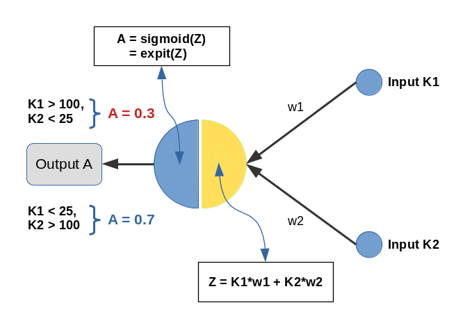
In this article series on a perceptron with only one computing neuron we saw that saturation effects of the sigmoid activation function can hamper gradient descent if input data on some features become too big and/or the initial weight distribution is not adapted to the number of input features. See:
We can remedy the first point by applying a normalization transformation to the input data before starting gradient descent. I showed the positive result of such a transformation for our perceptron with a rather specific set of input data in the last article:
At that time we used the “StandardScaler” provided by Scikit-Learn. In this article we shall instead use an instance of the “Normalizer” class for scaling. With “Normalizer” you have to be a bit careful how you use its interface. We shall apply “Normalizer in two different ways. Besides having some fun with the outcome, we will also learn that the shape of the clusters in which the input samples may be arranged in feature space should be taken into account before normalizing ahead of classification tasks. Which may be difficult in multiple dimensions … but it brings us to the general idea of identifying a method of cluster identification ahead of classification training with gradient descent.
How does the “Normalizer” work?
Let us offer a “Normalizer”-instance an input array “ay_in” with 2 rows and 4 columns for each row. The shape of “ay_in” is (2,4). The first row “s1” shall have elements like s1=[4, 1, 2, 2]. Then Normalizer will then calculate a L2-norm value for the column data of our specific row as
L2([4, 1, 2, 2]) = sqrt(4**2 + 1**2 + 2**2 + 2**2) = 5
=> s1_trafo = [4/L2, 1/L2, 2/L2, 2/L2] = [0.8, 0.2, 0.4, 0.4].
I.e., all columns in one row are multiplied by one common factor determined as the L2-norm of the column data of the sample. Note again: Each row is treated separately. So, an array as
[
  [1, 3, 9, 3],
  [5, 7, 5, 1]
]
will be transformed to
  [0.1,, 0.3, 0.9, 0.3],
  [0.5, 0.7, 0.5, 0.1]
]
How can we make use of this for our perceptron samples?
Standard scaling per feature with Normalizer
A first idea is that we could scale the data of all samples for our perceptron separately per feature; i.e. we collect the data-values of all M samples for “feature 1” in an array and offer it as the first row of an array to Normalizer, plus a row with all the data values for “feature 2”, …. and so on.
If we had M samples and N features we would present an array with shape (N, M) to “Normalizer”. In our simple perceptron experiment this is equivalent to scaling data of an array where the two rows are defined by our K1 and K2-input arrays => ay_K = [ li_K1, li_K2 ].
What would the outcome of such a scaling be?
A constant factor per feature determined by the L2-norm of all samples’ values for the chosen feature brings all values safely down into an interval of [-1, 1]. But this also means that the maximum value of all samples for a specific feature determines the scale.
Then so called “outliers”, i.e. samples whose values are far away from the average values of the samples, would have a major
impact. So “Normalizer”-Scaling is especially helpful, if the values per feature are limited by principle reasons. Note that this is e.g. the case with RGB-color or gray-scale values! Note also that the possible impact of outliers is also relevant for other normalizers as the “MinMaxNormalizer” of SciKit-Learn.
Although the scaling factors will be different per feature I would like to point out another aspect of scaling by a constant factor per feature over all samples: Such a transformation keeps up at least some structural similarity of the sample distribution in the feature space.
Scaling features per sample with Normalizer (?)
A different way of applying “Normalizer” would be to use the transformed array “ay_K.T” as input: For M samples and N features we would then present an array with shape (M, N) to a Normalizer instance. Its algorithm would then scale across the features of each sample. If we interpret a specific sample as a vector in the feature space then the L2-norm corresponds naturally to the length of this vector. Meaning: Normalizer would scale each sample by its vector length.
Two questions before experimenting
The two possible application methods for Normalizer lead directly to two questions for our simple test setup in a 2-dim feature space:
- How will lines of equal cost values (i.e. cost or loss contours) for our sigmoid-based loss function look like in the {K1, K2}-space after scaling a bunch of N (K1, K2)-datapoints with Normalizer per feature? I.e., if and when should we present an array of feature values with shape (N,M)?
- What would happen instead if we scaled each input sample individually across its features? I.e., what happens in a situation with M samples and N features and we feed “Normalizer” with an array (of the same feature values) which has a shape (N,M) instead of (M,N)?
I guess a “natural talent” on numbers as Mr Trump could give the answers without hesitation 🙂 . As we certainly are below the standards of the “genius” Mr Trump (his own words on multiple occasions) we shall pick the answers from plots below before we even try a deeper reasoning.
Application of “Normalizer” separately to the feature data of all batch samples
As you remember from the first article of this series our input batch contained samples (K1, K2) with values for K1 and K2 given by two 1-dim arrays :
li_K1 = [200.0,   1.0, 160.0,  11.0, 220.0,  11.0, 120.0,  22.0, 195.0,  15.0, 130.0,   5.0, 185.0,  16.0]
li_K2 = [ 14.0, 107.0,  10.0, 193.0,  32.0, 178.0,   2.0, 210.0,  12.0, 134.0,  15.0, 167.0,  10.0, 229.0]
The standard scaling application of Normalizer can be coded explicitly as (see the code given in the last article):
    rg_idx = range(num_samples)
    if scale_method == 0:
        shape_input = (2, num_samples)
        ay_K = np.zeros(shape_input)
        for idx in rg_idx:
            ay_K[0][idx] = li_K1[idx]
            ay_K[1][idx] = li_K2[idx]
        scaler = Normalizer()
        ay_K = scaler.fit_transform(ay_K)
        for idx in rg_idx:
            ay_K1[idx] = ay_K[0][idx]
            ay_K2[idx] = ay_K[1][idx]
        scaling_fact_K1 = ay_K1[0] / li_K1[0]
        scaling_fact_K2 = ay_K2[0] / li_K2[0]
        print(ay_K1)
        print("\n")
        print(ay_K2)
However, a much faster form, which avoids the explicit Python loop, is given by:
ay_K= np.vstack( (li_K1, li_K2) )
ay_K = scaler.fit_transform(ay_K)
ay_K1, ay_K2 = ay_K
scaling_fact_K1 = ay_K1[0] / li_K1[0]
scaling_fact_K2 = ay_K2[0] / li_K2[0]
Here OpenBlas helps 🙂 .
In contrast to other scalers we need to save and keep the
factors by which we transform the various feature data by ourselves somewhere. (This is clear as “Normalizer” calculates a different factor for each feature.) So, we change our Jupyter cell code for scaling to:
# ********
# Scaling
# ********

b_scale = True
scale_method = 0
# 0: Normalizer (standard), 1: StandardScaler, 2. By factor, 3: Normalizer per pair
# 4: Min_Max, 5: Identity (no transformation) - just there for convenience

shape_ay = (num_samples,)
ay_K1 = np.zeros(shape_ay)
ay_K2 = np.zeros(shape_ay)

# apply scaling
if b_scale:
    # shape_input = (num_samples,2)
    rg_idx = range(num_samples)
    if scale_method == 0:
        ay_K = np.vstack( (li_K1, li_K2) )
        print("ay_k.shape = ", ay_K.shape)
        scaler = Normalizer()
        ay_K = scaler.fit_transform(ay_K)
        ay_K1, ay_K2 = ay_K
        scaling_fact_K1 = ay_K1[0] / li_K1[0]
        scaling_fact_K2 = ay_K2[0] / li_K2[0]
        print("\nay_K1 = \n", ay_K1)
        print("\nay_K2 = \n", ay_K2)
        print("\nscaling_fact_K1: ", scaling_fact_K1, ", scaling_fact_K2: ", scaling_fact_K2)

    elif scale_method == 1:
        ay_K = np.column_stack((li_K1, li_K2))
        scaler = StandardScaler()
        ay_K = scaler.fit_transform(ay_K)
        ay_K1, ay_K2 = ay_K.T

    elif scale_method == 2:
        dmax = max(li_K1.max() - li_K1.min(), li_K2.max() - li_K2.min())
        ay_K1 = 1.0/dmax * li_K1
        ay_K2 = 1.0/dmax * li_K2
        scaling_fact_K1 = ay_K1[0] / li_K1[0]
        scaling_fact_K2 = ay_K2[0] / li_K2[0]

    elif scale_method == 3:
        ay_K = np.column_stack((li_K1, li_K2))
        scaler = Normalizer()
        ay_K = scaler.fit_transform(ay_K)
        ay_K1, ay_K2 = ay_K.T

    elif scale_method == 4:
        ay_K = np.column_stack((li_K1, li_K2))
        scaler = MinMaxScaler()
        ay_K = scaler.fit_transform(ay_K)
        ay_K1, ay_K2 = ay_K.T

    elif scale_method == 5:
        ay_K1 = li_K1
        ay_K2 = li_K2


# Get overview over costs on weight-mesh
#wm1 = np.arange(-5.0,5.0,0.002)
#wm2 = np.arange(-5.0,5.0,0.002)
wm1 = np.arange(-5.5,5.5,0.002)
wm2 = np.arange(-5.5,5.5,0.002)
W1, W2 = np.meshgrid(wm1, wm2)
C, li_C_sgl = costs_mesh(num_samples = num_samples, W1=W1, W2=W2, li_K1 = ay_K1, li_K2 = ay_K2, \
                               li_a_tgt = li_a_tgt)


C_min = np.amin(C)
print("\nC_min = ", C_min)
IDX = np.argwhere(C==C_min)
print ("Coordinates: ", IDX)
# print(IDX.shape)
# print(IDX[0][0])
wmin1 = W1[IDX[0][0]][IDX[0][1]]
wmin2 = W2[IDX[0][0]][IDX[0][1]]
print("Weight values at cost minimum:",  wmin1, wmin2)

# Plots
# ******
fig_size = plt.rcParams["figure.figsize"]
#print(fig_size)
fig_size[0] = 16; fig_size[1] = 16

fig3 = plt.figure(3); fig4 = plt.figure(4)

ax3 = fig3.gca(projection='3d')
ax3.get_proj = lambda: np.dot(Axes3D.get_proj(ax3), np.diag([1.0, 1.0, 1, 1]))
ax3.view_init(20,135)
ax3.set_xlabel('w1', fontsize=16)
ax3.set_ylabel('w2', fontsize=16)
ax3.set_zlabel('Total costs', fontsize=16)
ax3.plot_wireframe(W1, W2, 1.2*C, colors=('green'))


ax4 = fig4.gca(projection='3d')
ax4.get_proj = lambda: np.dot(Axes3D.get_proj(ax4), np.diag([1.0, 1.0, 1, 1]))
ax4.view_init(25,135)
ax4.set_xlabel('w1', fontsize=16)
ax4.set_ylabel('w2', fontsize=16)
ax4.set_zlabel('Single costs', fontsize=16)
ax4.plot_wireframe(W1, W2, li_C_sgl[0], colors=('blue'))
#ax4.plot_wireframe(W1, W2, li_C_sgl[1], colors=('red'))
ax4.plot_wireframe(W1, W2, li_C_sgl[5], colors=('orange'))
#ax4.plot_wireframe(W1, W2, li_C_sgl[6], colors=('yellow'))
#ax4.plot_wireframe(W1,
W2, li_C_sgl[9], colors=('magenta'))
#ax4.plot_wireframe(W1, W2, li_C_sgl[12], colors=('green'))

plt.show()
Ok, lets apply the “Normalizer” to our input samples. We get:
ay_K1 =
 [0.42786745 0.00213934 0.34229396 0.02353271 0.47065419 0.02353271
 0.25672047 0.02995072 0.41717076 0.03209006 0.27811384 0.01069669
 0.39577739 0.0342294 ]

ay_K2 =
 [0.02955501 0.22588473 0.02111072 0.40743694 0.06755431 0.37577085
 0.00422214 0.44332516 0.02533287 0.28288368 0.01477751 0.35254906
 0.02111072 0.48343554]

scaling_fact_K1:  0.0021393372268854655 , scaling_fact_K2:  0.0021110722130092533
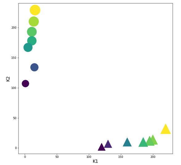
How do the transformed data points look like in the {K1, K2}-feature-space? See the plot:
Structurally very like the original; but with values reduced to [0,1]. This was to be expected.
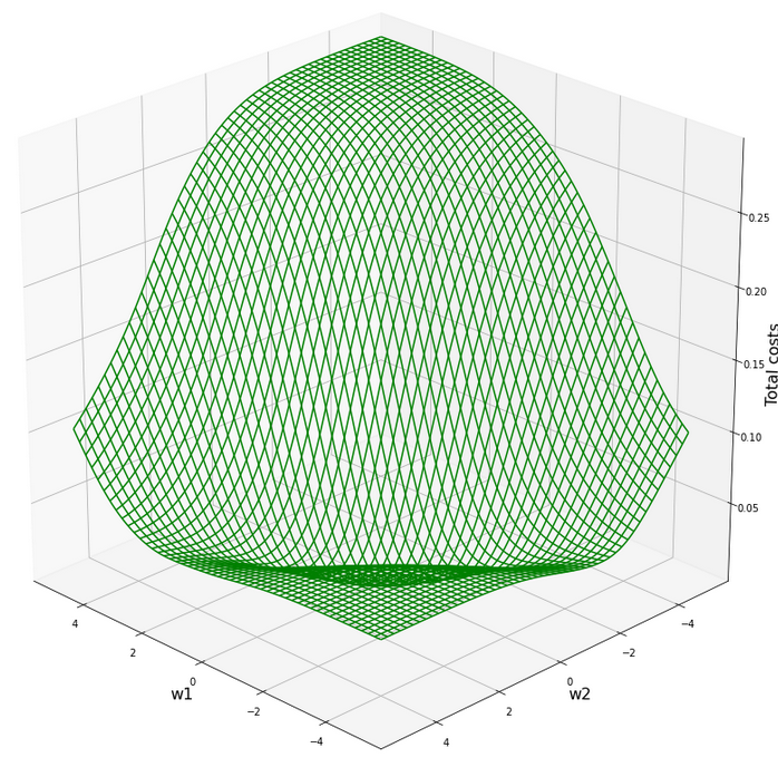
The cost hyperplane for the data normalized “per feature“
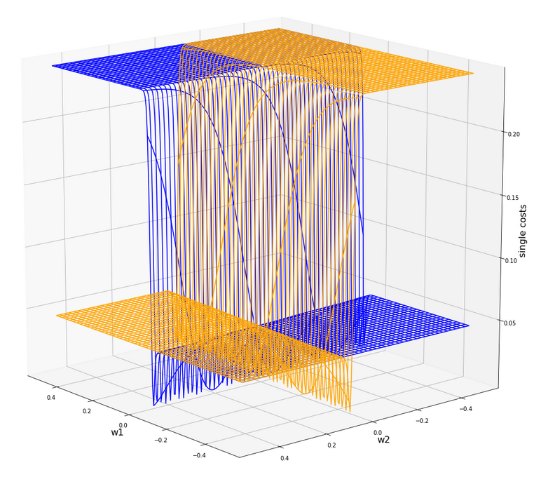
After the transformation of the sample data the cost hyperplane over the {w1, w2}-space looks as follows:
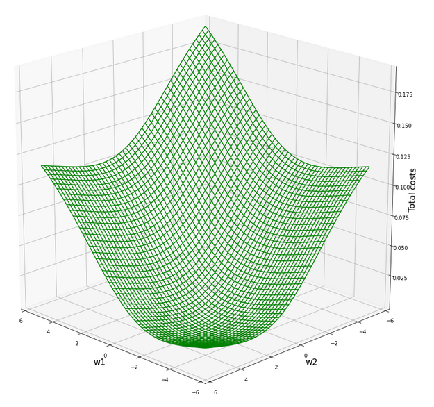
We see a clear minimum; it does, however, not appear as pronounced as for the StandardScaler, which we applied in the last article.
But: There are no side valleys with small gradients at the end of the steep slope area. This means that a path into a minimum will probably look a bit different compared to a path on the hyperplane we got with the “StandardScaler”.
Our mesh in the {w1, w2}-space indicates the following position of the minimum:
C_min =  0.0006350159045771724
Coordinates:  [[3949 1542]]
Weight values at cost minimum: -2.4160000000003397 2.39799999999913
Gradient descent results after normalization per feature with “Normalizer”
With our gradient descent method and the following run-parameters
w1_start = -0.20, w2_start = 0.25 eta = 0.2, decrease_rate = 0.00000001, num_steps = 2500
we get the following result of a run which explores both stochastic and batch gradient descent:
Stoachastic Descent
          Kt1       Kt2     K1     K2  Tgt       Res       Err
0   0.427867  0.029555  200.0   14.0  0.3  0.276365  0.078783
1   0.002139  0.225885    1.0  107.0  0.7  0.630971  0.098613
2   0.342294  0.021111  160.0   10.0  0.3  0.315156  0.050519
3   0.023533  0.407437   11.0  193.0  0.7  0.715038  0.021483
4   0.470654  0.067554  220.0   32.0  0.3  0.273924  0.086920
5   0.023533  0.375771   11.0  178.0  0.7  0.699320  0.000971
6   0.256720  0.004222  120.0    2.0  0.3  0.352075  0.173584
7   0.029951  0.443325   14.0  210.0  0.7  0.729191  0.041701
8   0.417171  0.025333  195.0   12.0  0.3  0.279519  0.068271
9   0.032090  0.282884   15.0  134.0  0.7  0.645816  0.077405
10  0.278114  0.014778  130.0    7.0  0.3  0.346085  0.153615
11  0.010697  0.352549    5.0  167.0  0.7  0.694107  0.008418
12  0.395777  0.021111  185.0   10.0  0.3  0.287962  0.040126
13  0.034229  0.483436   16.0  229.0  0.7  0.745803  0.065432

Batch Descent
          Kt1       Kt2     K1     K2  Tgt       Res       Err
0   0.427867  0.029555  200.0   14.0  0.3  0.276360  0.078799
1   0.002139  0.225885    1.0  107.0  0.7  0.630976  0.098606
2   0.342294  0.021111  160.0   10.0  0.3  0.315152  0.050505
3   0.023533  0.407437
11.0  193.0  0.7  0.715045  0.021493
4   0.470654  0.067554  220.0   32.0  0.3  0.273919  0.086935
5   0.023533  0.375771   11.0  178.0  0.7  0.699326  0.000962
6   0.256720  0.004222  120.0    2.0  0.3  0.352072  0.173572
7   0.029951  0.443325   14.0  210.0  0.7  0.729198  0.041711
8   0.417171  0.025333  195.0   12.0  0.3  0.279514  0.068287
9   0.032090  0.282884   15.0  134.0  0.7  0.645821  0.077398
10  0.278114  0.014778  130.0    7.0  0.3  0.346081  0.153603
11  0.010697  0.352549    5.0  167.0  0.7  0.694113  0.008410
12  0.395777  0.021111  185.0   10.0  0.3  0.287957  0.040142
13  0.034229  0.483436   16.0  229.0  0.7  0.745810  0.065443

Total error stoch descent:  0.06898872490256348
Total error batch descent:  0.06899042421795792
Good! Seemingly we got some convergence in both cases. The overall “accuracy” achieved on the training set is even a bit better than for the “StandardScaler”. And:
Final (w1,w2)-values stoch : ( -2.4151 ,  2.3977 )
Final (w1,w2)-values batch : ( -2.4153 ,  2.3976 )
This fits very well to the data we got from our mesh analysis of the cost hyperplane!
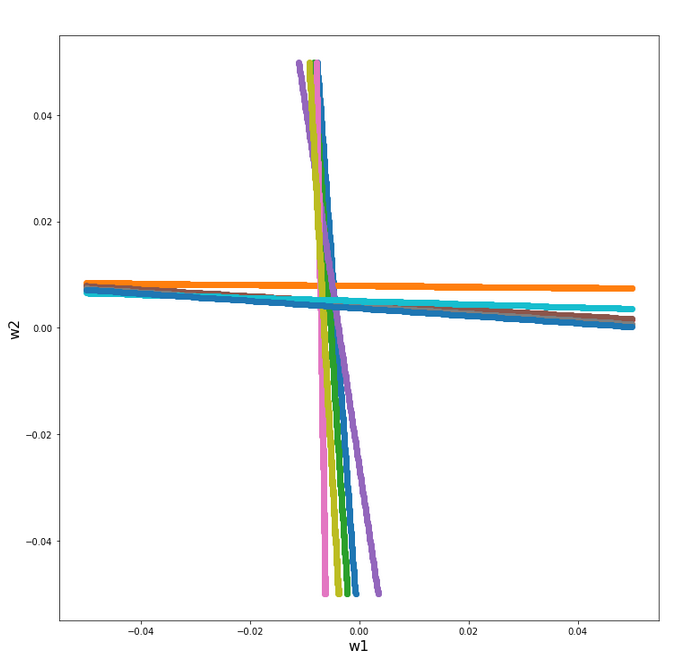
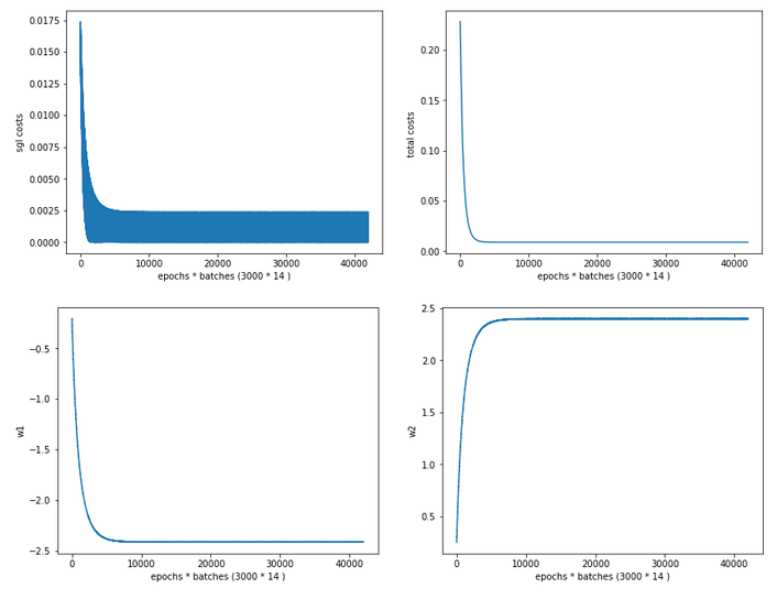
Regarding the evolution of the costs and the weights we see a slightly different picture than with the “StandardScaler”:
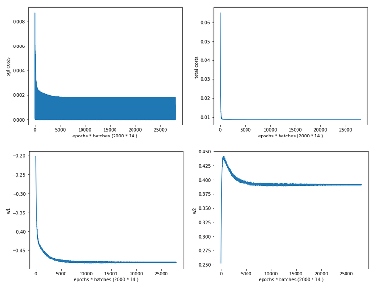
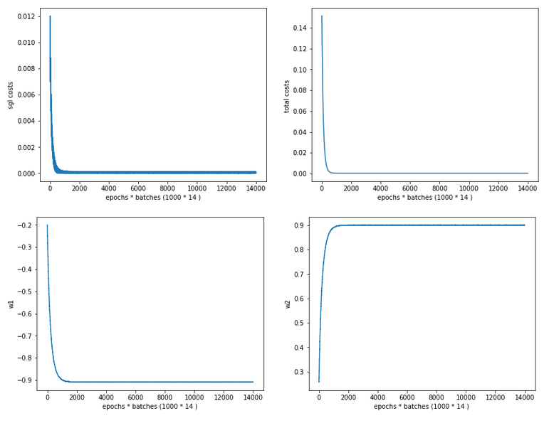
Cost and weight evolution during stochastic gradient descent
and:
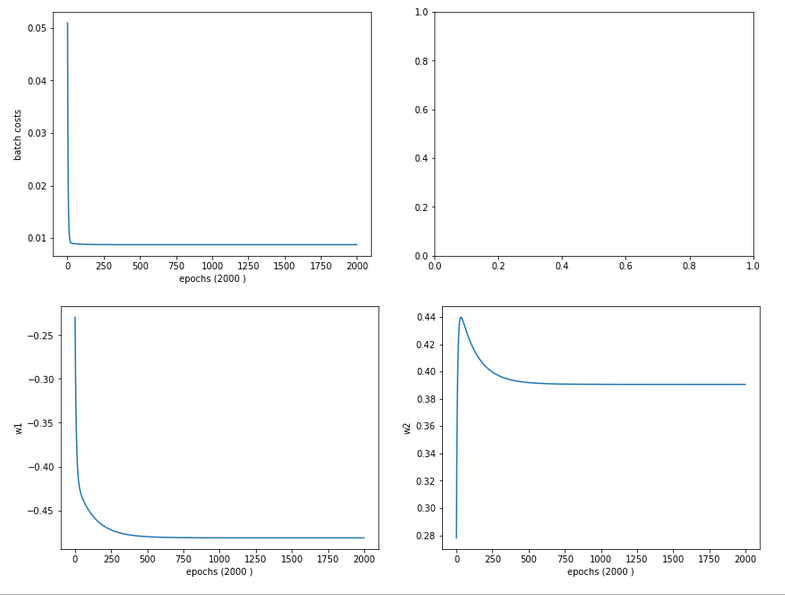
Cost and weight evolution during batch gradient descent
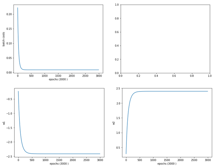
From the evolution of the weight parameters we can assume that gradient descent moved along a direct path into the cost minimum. This fits to the different shape of the cost hyperplane in comparison with the hyperplane we got after the application of the “StandardScaler”.
Predicted contour and separation lines in the {K1, K2}-plane after feature-scaling with “Normalizer”
We compute the contour lines of the output A of our solitary neuron (see article 1 of this series) with the following code:
# ***********
# Contours
# ***********
from matplotlib import ticker, cm

# Take w1/w2-vals from above w1f, w2f
w1_len = len(li_w1_ba)
w2_len = len(li_w1_ba)
w1f = li_w1_ba[w1_len -1]
w2f = li_w2_ba[w2_len -1]

def A_mesh(w1,w2, Km1, Km2):
    kshape = Km1.shape
    A = np.zeros(kshape)

    Km1V = Km1.reshape(kshape[0]*kshape[1], )
    Km2V = Km2.reshape(kshape[0]*kshape[1], )
    print("km1V.shape = ", Km1V.shape, "\nkm1V.shape = ", Km2V.shape )

    # scaling trafo
    if scale_method == 0:
        Km1V = scaling_fact_K1 * Km1V
        Km2V = scaling_fact_K2 * Km2V
        KmV = np.vstack( (Km1V, Km2V) )
        KmT = KmV.T
    else:
        KmV = np.column_stack((Km1V, Km2V))
        KmT = scaler.transform(KmV)

    Km1T, Km2T = KmT.T
    Km1TR = Km1T.reshape(kshape)
    Km2TR = Km2T.reshape(kshape)
    print("km1TR.shape = ", Km1TR.shape, "\nkm2TR.shape = ", Km2TR.shape )


    rg_idx = range(num_samples)
    Z      = w1 * Km1TR + w2 * Km2TR
    A = expit(Z)
    return A

#Build K1/K2-mesh
minK1, maxK1 = li_K1.min()-20, li_K1.max()+20
minK2, maxK2 = li_K2.min()-20, li_
K2.max()+20
resolution = 0.1
Km1, Km2 = np.meshgrid( np.arange(minK1, maxK1, resolution),
                        np.arange(minK2, maxK2, resolution))

A = A_mesh(w1f, w2f, Km1, Km2 )
print("A.shape = ", A.shape)

fig_size = plt.rcParams["figure.figsize"]
#print(fig_size)
fig_size[0] = 14
fig_size[1] = 11
fig, ax = plt.subplots()
cmap=cm.PuBu_r
cmap=cm.RdYlBu
#cs = plt.contourf(X, Y, Z1, levels=25, alpha=1.0, cmap=cm.PuBu_r)
cs = ax.contourf(Km1, Km2, A, levels=25, alpha=1.0, cmap=cmap)
cbar = fig.colorbar(cs)
N = 14
r0 = 0.6
x = li_K1
y = li_K2
area = 6*np.sqrt(x ** 2 + y ** 2)  # 0 to 10 point radii
c = np.sqrt(area)
r = np.sqrt(x ** 2 + y ** 2)
area1 = np.ma.masked_where(x < 100, area)
area2 = np.ma.masked_where(x >= 100, area)
ax.scatter(x, y, s=area1, marker='^', c=c)
ax.scatter(x, y, s=area2, marker='o', c=c)
# Show the boundary between the regions:
ax.set_xlabel("K1", fontsize=16)
ax.set_ylabel("K2", fontsize=16)
Please note the differences in how we handle the creation of the array “KmT” with the transformed data for “scale_method=0”, i.e. “Normalizer”, in comparison to other methods.
Here is the result:
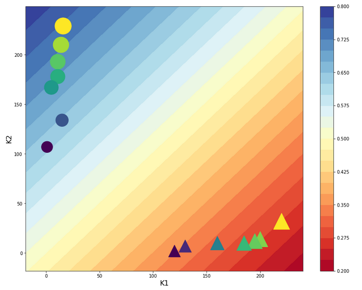
Looks very similar to our plot for the StandardScaler in the last article – but with a slight shift on the K1-axis. So, the answer to our first question is: The contour lines are straight diagonal lines!
This is a direct result of the equations
expit(z) = E_z = const. => z = const. => w1*f1*K1 + w2*f2*K2 = C_z =>
K2 = C_k -fact*K1
The last one is nothing but an equation for a straight line. As “factor” is a constant, the angle α with the K1-axis remains the same for different E_z and C_k, i.e. we get parallel lines. If “fact = “-w1*f1/w2*f2 ≈ 1 = tan(α)” we get almost a 45°ree;-angle α. Let us see in our case : w1 = -2.4151 , w2 = 2.3977, f1 = 0.00214, f2 = 0.00211 => fact = 1.0215. This explains our plot.
“Normalizer” used per sample
Now we scale the (K1, K2) coordinates in feature space of each single sample with the Normalizer. I.e. we scale K1 and K2 for each individual sample by a common factor 1/sqrt(K1**2 + K2**2). Meaning: No scaling with a common factor per feature over all samples; instead scaling of the features per sample. As already said: If we regard K1 and K2 as coordinates of a vector then we scale the distance of vectors end point radially to the origin of the coordinate system down to a length of 1.
Thus: After this normalization transformation we expect that our points are located on a unit circle! Note, however, that our transformation keeps up the angular distance of all data points. By “angular distance” for two selected points we mean the difference of the angles of these data points with e.g. the K1-axis.
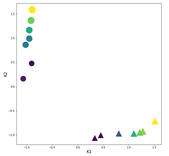
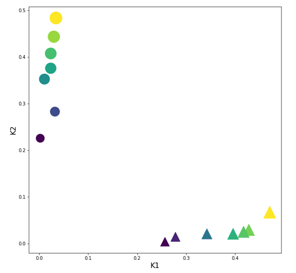
Let us look at the transformed sample points in the {K1, K2}-plane:
Ok, our transformation has done a more pronounced “clustering” for us. Our transformed clusters are even more clearly separated from each other than before!
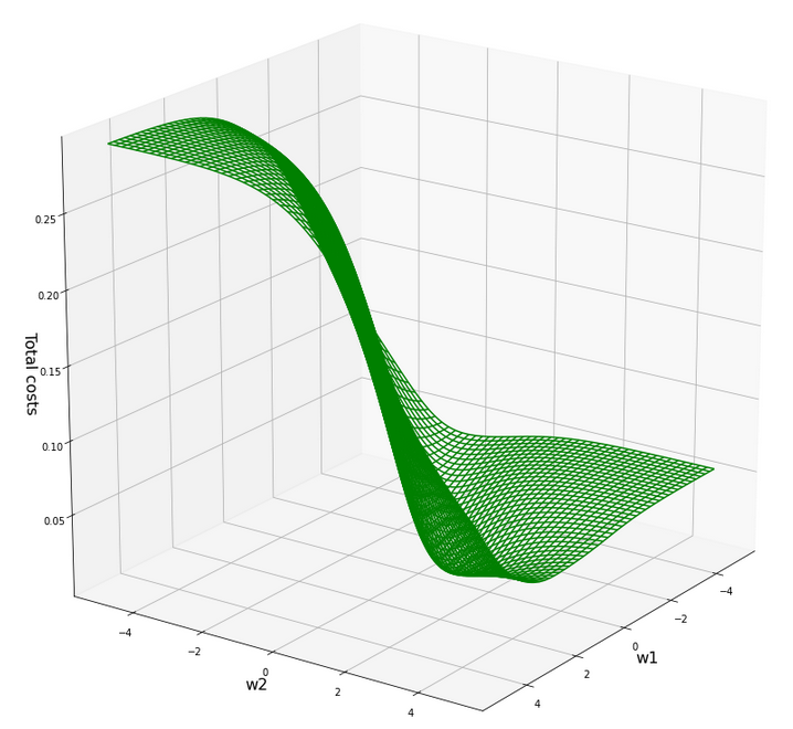
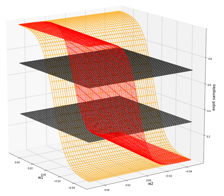
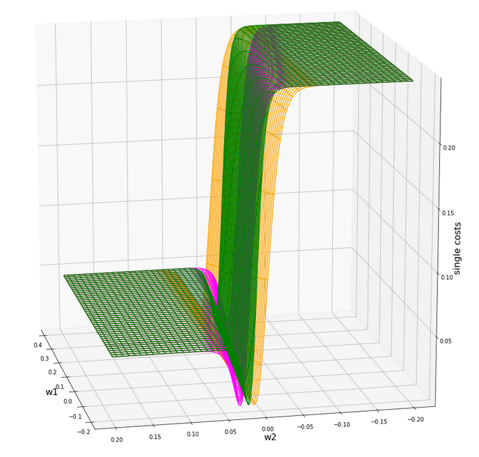
What does this mean for our cost hyperplane in the {w1, w2}-space? Well, here is a mesh-plot:
Cost hyperplane of
the data scaled per sample by “Normalizer” in the {w1, w2}-space
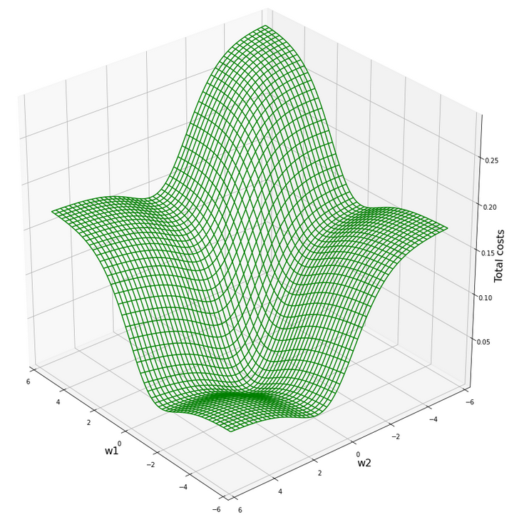
According to our mesh the minimum is located at:
C_min =  2.2726781812937556e-05
Coordinates:  [[3200 2296]]
Weight values at cost minimum: -0.9080000000005057 0.8999999999992951
Comparison of the cost hyperplane with center of the original hyperplane for the unscaled batch data
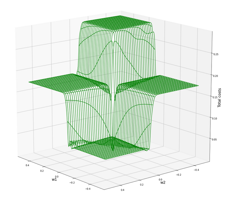
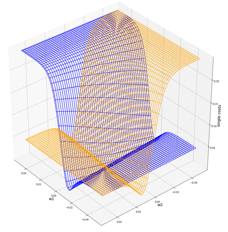
Now comes a really funny point: Do you remember that we have gotten a similar plot before? Actually, we did when we looked at a tiny surroundings of the center of the cost hyperplane of the original unscaled data in the first article of this series:
Cost hyperplane at the center of the original unscaled input data in the {w1, w2}-space?
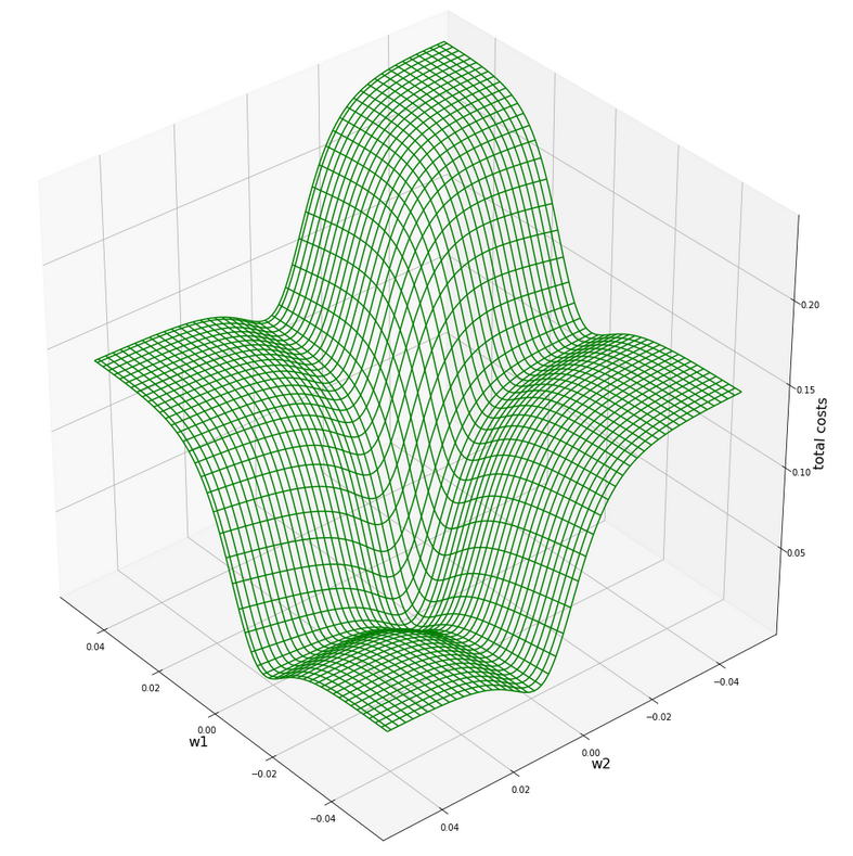
A somewhat different viewing angle – but the similarity is obvious. Note however the very different scales of the (w1, w2)-values compared to the version of the scaled data.
How do we explain this similarity? Part of the answer lies in the fact that the total costs of the batch are dominated by those samples who have the biggest coordinate values, i.e. of those points where either K1 or K2 is biggest. Now, these points were very close to each other in the original data set. Now, for such points a centric stretch by a factor of around 1/200 would require a centric stretch (but now an expansion!) for the (w1, w2)-data with a reciprocate factor if we wanted to reproduce the same cost values. Reason: Linear coupling w1*K1+w2*K2! You compensate a constant factor in the {K1,K2}-space by its reciprocate one in the {w1, W2}-space!
But that is more or less what we have done by our somewhat strange application of the “Normalizer”! At least almost … Fun, isn’t it?
Gradient descent after sample-wise (!) normalization by the “Normalizer”
The clearer separation of the clusters in the {K1, K2}-space after separation and a well formed cost hyperplane over the {w1, w2}-space should help us a bit with our gradient descent. We set the parameters of a gradient descent run to
w1_start = -0.20, w2_start = 0.25 eta = 0.2, decrease_rate = 0.00000001, num_steps = 1000
and get:
Stoachastic Descent
          Kt1       Kt2     K1     K2  Tgt       Res       Err
0   0.997559  0.069829  200.0   14.0  0.3  0.300715  0.002383
1   0.009345  0.999956    1.0  107.0  0.7  0.709386  0.013408
2   0.998053  0.062378  160.0   10.0  0.3  0.299211  0.002629
3   0.056902  0.998380   11.0  193.0  0.7  0.700095  0.000136
4   0.989586  0.143940  220.0   32.0  0.3  0.316505  0.055018
5   0.061680  0.998096   11.0  178.0  0.7  0.699129  0.001244
6   0.999861  0.016664  120.0    2.0  0.3  0.290309  0.032305
7   0.066519  0.997785   14.0  210.0  0.7  0.698144  0.002652
8   0.998112  0.061422  195.0   12.0  0.3  0.299019  0.003269
9   0.111245  0.993793   15.0  134.0  0.7  0.688737  0.016090
10  0.998553  0.053768  130.0    7.0  0.3  0.297492  0.008360
11  0.029927  0.999552    5.0  167.0  0.7  0.705438  0.007769
12  0.998542  0.053975  185.0   10.0  0.3  0.297533  0.008223
13  0.069699  0.997568   16.0  229.0  0.7  0.697493  0.003581

Batch Descent
          Kt1       Kt2     K1     K2  Tgt       Res       Err
0   0.997559  0.069829  200.0   14.0  0.3  0.300723  0.002409
1   0.009345  0.999956    1.0
107.0  0.7  0.709388  0.013411
2   0.998053  0.062378  160.0   10.0  0.3  0.299219  0.002604
3   0.056902  0.998380   11.0  193.0  0.7  0.700097  0.000139
4   0.989586  0.143940  220.0   32.0  0.3  0.316513  0.055044
5   0.061680  0.998096   11.0  178.0  0.7  0.699131  0.001241
6   0.999861  0.016664  120.0    2.0  0.3  0.290316  0.032280
7   0.066519  0.997785   14.0  210.0  0.7  0.698146  0.002649
8   0.998112  0.061422  195.0   12.0  0.3  0.299027  0.003244
9   0.111245  0.993793   15.0  134.0  0.7  0.688739  0.016087
10  0.998553  0.053768  130.0    7.0  0.3  0.297500  0.008335
11  0.029927  0.999552    5.0  167.0  0.7  0.705440  0.007771
12  0.998542  0.053975  185.0   10.0  0.3  0.297541  0.008198
13  0.069699  0.997568   16.0  229.0  0.7  0.697495  0.003578

Total error stoch descent:  0.011219103621660675
Total error batch descent:  0.01121352661948904
Well, this is a almost perfect result on the training set; just between 1% and 3% deviation from the aspired output values. We have obviously found something new! Before, we always had deviations up to 15% or even 20% in the prediction for some of the data samples in our training set.
The final values of the weights become:
Final (w1,w2)-values stoch : ( -0.9093 ,  0.9009 )
Final (w1,w2)-values batch : ( -0.9090 ,  0.9009 )
Also very perfect. You should not forget – we worked with just 14 samples and 1 neuron.
The evolution data look like:
Cost and weight evolution during stochastic gradient descent
and:
Cost and weight evolution during batch gradient descent
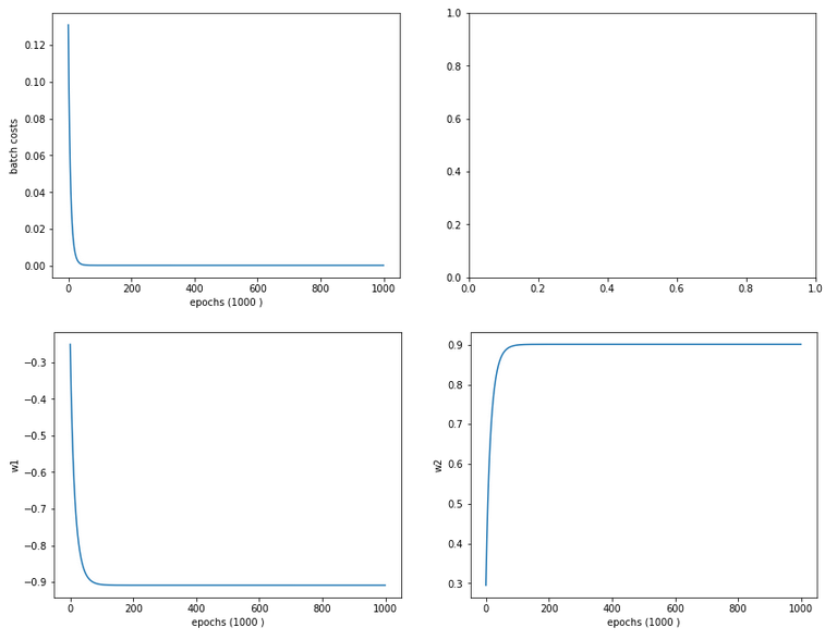
Smooth development; fast convergence!
Separation lines in the {K1, K2}-space after “per sample”-normalization with “Normalizer”
Now we turn to the answer to the second question we asked above: What changes regarding the separation or contour lines of the output values of our solitary neuron? Well as in our last article, we are interested in the output of our neuron after the normalization transformation of the data. I.e. we are on the search for contour lines, which we get for those points in the original {K1, K2}-space for which the sigmoid function produces a constant after transformation.
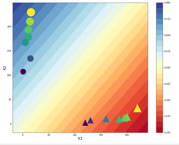
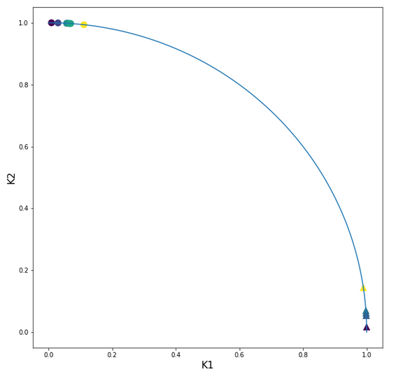
Here is the plot:
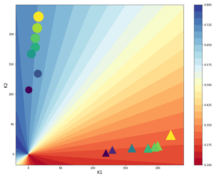
Ooops, now we get a real difference. The contour curves are straight lines, but now directed radially outwards from the origin into the {K1, K2}-space! You see in addition that most of the data points are located very close to the lines for the set values A=0.3 and A=0.7!
We also get a very clear separation line close to diagonal at 45°ree;. A few comments on this finding:
The subdivision of the {K1, K2}-plane into sectors is very appropriate for clusters with data which show a tendency of a constant ration between the K1 and K2 values or clusters with a narrow extension
in both directions. Note, however, that if we had two clusters at different radial distances but at roughly the same angle our present Normalizer transformation per sample would not have been helpful but disastrous regarding separation. So: The application of special normalization procedures ahead of classification training must be done with a feeling or insight into the clustering structure in the feature space.
Why radial contour lines?
What are the contour lines in the original {K1, K2}-space which produce the same output A for the transformed data? If we name the transformed (K1, K2) values by (k1, k2) we get in our case
k1 = K1/(K1**2 + K2**2)
k2 = K2/(K1**2 + K2**2)
So, we are looking for points in the {K1, K2}-space for which the equation
expit(w1*k1+ w2*k2) = const.
We now have to show that this is fulfilled for lines that have the property K2/K1 = tan(alpha) with alpha = const.. The proof is a small algebraic exercise, which I leave to my readers. Of course a genius like Mr Trump would give a direct answer based on the transformation properties itself: We just eliminated the radial distance to the origin as a feature! I leave it up to you which way of reasoning you want to go.
Clustering ahead of gradient descent?
Our very specific way of using the “Normalizer” has led us to a clearer clustering after the scaling transformation. This gives rise to a fundamental idea:
What if you could use some method to detect clusters in the distribution of datapoints in feature space ahead of gradient decent?
But, on basis of what input or feature data then? Well, we could use some norm (as L2) to describe the distance of the data points from the centers of the different identified clusters as the new features! If we knew the centers of the clusters such an approach could have a potential advantage: It would set the the number of the new features to the number of the identified clusters. And this number could be substantially smaller than the number of originally features Why? Because in general not all features may be independent of each other and not all may be of major importance for the classification and cluster membership.
We shall follow this idea in my other series on a real MLP and MNIST in more detail.
Conclusion
In this article we studied the application of the “Normalizer” offered by Scikit-Learn in two different ways to a training scenario for a one neuron perceptron and data with two input features (only). Normally we would apply “Normalizer” such that we would scale the data of all samples for each feature separately. And use the found stretching factors later on on new data points for which we want to make a classification prediction.
We saw that such a transformation roughly kept up the structure of the datapoint distribution in the {K1, K2}-fature-space. Scaling into an interval [-1, 1] had a major and healthy impact on the structure of the cost hyperplane in the {w1, w2}-weight-space. This helped us to perform a smooth gradient descent calculation.
Then we performed an application of “Normalizer” per sample. This corresponded to a radial stretch of all datapoints down to a unit cycle, whilst keeping up the values of the angles. We got a more structured cost hyperplane afterwards and a stronger clustering effect in the special case of our transformed data distribution in feature space. This helped gradient descent quite a lot: We could classify our data much better according to our discrimination prescription A=0.3 vs. A=0.7.
Our transformation also had the interesting effect of sub-dividing the feature space into radial sectors instead of parallel stripes. This would be helpful in case of data clusters with a certain radial elongation in the feature space but a clear difference and separation in angle. Such data do indeed exist – just think of the distribution of stars or
microwave radiation clusters on the nightly sky sphere. At least in the latter case the radial distance of the sources may be of minor importance: You do not need radial distance information to note a concentration in a region which we call “milky way”!
What we actually did with our special normalization was to indirectly eliminate the radial distance information hidden in our (K1, K2)-data. We could also have calculated the angle (or a function of it) directly and thrown away all other information. If we had done so, we would have reduced our 2-dim the feature space to just one dimension! We saw this directly on the plot of the contour lines! Thus: It would have been much more intelligent, if we had used our transformation in a slightly modified form, determined just the angle of our data-points directly and uses these data as the only feature guiding gradient descent.
This led us to the idea that a clear identification of clusters by some appropriate method before we start a gradient descent analysis might be helpful for classification tasks.
This in turn triggers the idea of a cluster detection in feature space – which itself actually is a major discipline of Machine Learning. An advantage of using cluster detection ahead of gradient descent would be the possible reduction of the number of input features for the artificial neural network. Take a look at a forthcoming article in my other series on a Multilayer Perceptron [MLP] in this blog for an application in combination with a MLP and the MNIST daset.
In the next article of this series on a minimalistic perceptron we shall add a bias neuron to the input layer and investigate the impact.