Some readers may remember a post series I have written in this blog about the reconstruction of human faces with a CNN-based Autoencoder. I could show that the information in the latent space of the Autoencoder is given in form of a core of a Multivariate Normal Distribution [MVN].
This did not surprise too much as there are good reasons to assume that facial features on average, but in particular across rather symmetric celebrity faces follow Gaussian distributions. Hundreds of encoded features together form a MVN-distribution in a latent space of hundreds of dimensions. The Encoder part of a CNN-based Autoencoder is a pattern extraction machine – and there is no simpler pattern in multiple dimensions than a (off-center) MVN! A MVN’s multidimensional and concentric contour surfaces are ellipsoids, which have an algebraic description in form of quadratic forms. In case of the MVN defined by the inverse of the covariance matrix.
During the named series, I have extensively used that fact that the projections of a multidimensional MVN down to a coordinate planes result in 2-dimensional bivariate MVNs. The elements of the (2×2)-covariance matrix of the various 2-dimensional projected distributions could simply be picked from (nxn) covariance matrix of the original MVN – by a simple selection process. I had taken this procedure as granted, as it had been claimed in some publications. And it worked very well … See e.g.
and links therein to other posts. The projection of course affects the (n-1)-dimensional ellipsoidal and concentric contour surfaces of a MVN and maps them onto (p-1)-dimensional contour ellipses of the projected 2-dimensional MVNs. For respective images see this post:
Last weeks I looked a bit deeper into the mathematics of orthogonal projections of multidimensional ellipsoids onto sub-spaces of the ℝn. It came a bit of a surprise to me that the math behind the projections of figures controlled by quadratic forms is relatively complicated. In the general case of the projection to a p-dimensional sub-space, the quadratic form matrix for the ellipsoidal hull of the projection image is a so called Schur complement of the original ellipsoid’s quadratic form matrix.
Fortunately, the relation between the inverse matrices of the quadratic forms for the ellipsoids could be established in a way that is fully consistent with the mapping of covariance matrices of MVNs and and related matrices of their projection images. However and in contrast to other publications, I found that a solid proof requires some Linear Algebra around Schur complements.
Readers interested in MVNs and their mathematical properties for statistical analysis e.g. in Machine Learning contexts may find detailed information in the following articles of mine:
Orthogonal projections of multidimensional ellipsoids
People doing Machine Learning [ML] experiments on their own Linux PCs or laptops know that the numerical training runs put a heavy load on the graphics cards and consume a lot of energy as a direct consequence. Especially in a hot summer like we have it in Germany right now, cooling of your systems may become a problem. And as energy has a high price tag here, any method to reduce the load and/or power consumption is welcome.
But I think that caring about energy consumption is a topic which we as a Linux and ML enthusiasts should keep in mind in general. Some big tech companies will probably not do it – as long as their money machinery works and as some heads follow fantasies about building small nuclear power plants for their big AI data centers. But we Opensource people would like to see more AI- and ML-services independent of the monopolists and their infrastructure, anyway. Not only for reasons of data and privacy protection.
As soon as we, however, proclaim and work for a development that favors local and resource optimized installations of AI and ML tools both for private people and companies, we have to care about side effects: We have to bring the energy consumption down for these many local installations substantially in parallel. Otherwise, centralized solutions may have a better energy efficiency than decentralized solutions.
For me as a retired person in Germany the general financial pressure is high enough to enforce a careful use of my private resources. With this post I want to draw your attention to two points which may help you, too, to save energy during your ML-experiments. (In addition to or aside of standard measures like saving certain model states during training runs to get better starting points for new runs.)
Working with Machine Learning and Deep Neural Networks not only requires GPU drivers, but in case of Nvidia GPUs also the installation of CUDA and cuDNN. This process is always a bit tricky as additional environment variables have to be set for IPython-based Jupyterlab or classic Jupyter Notebook. On an Opensuse system one must in addition take care of the right settings in /etc/alternatives.
I hope this helps people who want to use Leap 15.5 for Machine Learning with Nvidia GPUs, Keras/Tensorflow 2 and Jupyterlab.
Important addendum 01/27/2024:
Although the combination of CUDA 12.3, cuDNN 8.9.7, Tensorflow 2.15 and Nvidia drivers 545.29.06 works regarding AI-models, there is another major problem:
Nvidia’s driver 545.29.06 is buggy – at least for Leap 15.5, KDE/Plasma with multiple screens. The bug affects Suspend-to-RAM. Suspend-to-RAM seems to work in the suspend phase, and the system also comes up afterward in a seemingly proper state of your KDE/Plasma interface (on your screens).
However, the problems begin when you want to change to another virtual screen via Ctrl-Alt-Fx. You wait and wait and wait … The same for changing the run-level or systemd target state or when you want to shut the system down. This makes Suspend-to-RAM with driver 545.29.06 impossible to use.
Recommendation:
If you have a working older Nvidia driver (e.g. a stable 535 version) do not change to 545.29.06. Unfortunately, it is a mess on a multiscreen Leap 15.5 system to return to an older driver version. The Nvidia community repository does not offer you a choice. (Why by the way ????). Downloading an older proprietary driver from Nvidia and trying to install it afterward on a console terminal (after having stopped X11 or Wayland) did not work in my case – the screens displaying the terminal changed their resolution and froze afterward. So, you may have to completely uninstall the present driver 545 completely, go back to standard VGA and then try to install an older driver via Nvidias install mechanism. As I said: It is a mess …
we have clarified some basic properties of shear transformations [SHT]. We got interested in this topic, because Autoencoders can produce latent multivariate normal vector distributions, which in turn result from linear transformations of multivariate standard normal distributions. When we want to analyze such latent vector distributions we should be aware transformations of quadratic forms. An important linear transformation is a shear operation. It combines aspects of scaling with rotations.
The objects we applied SHTs to were so far only squares and cubes. Both (discrete) rotational and plane symmetries of the squares and cubes were broken by SHTs. We also saw that this symmetry breaking could not be explained by a pure scaling operation in another rotated Euclidean Coordinate System [ECS]. But cubes do not have a continuous rotational symmetry. The distances of surface points of a cube to its symmetry center show no isotropy.
However, already in the first post when we superficially worked with Blender we got the impression that the shearing of a sphere seemed to produce a figure with both plane and discrete rotational symmetries – namely ellipsoids, wich appeared to be rotated. We still have to prove this, mathematically. With this post we move a first step in this direction: We will apply a shear operation to a 2D-body with perfect continuous rotational symmetry in all directions, namely a circle. A circle is a special example of a quadratic form (with respect to the vector component values). We center our Euclidean Coordinate System [ECS] at the center of the circle. We know already that this point remains a fix-point of our transformations. As in the previous post I use Python and Matplotlib to produce visual results. But we support our impression also by some simple math.
We first check via plotting that the shear operations move an extremal point of the circle (with respect to the y-coordinate) along a line ymax = const. (Points of other layers for other values yl = const also move along their level-lines.) We then have to find out whether the produced figure really is an ellipse. We do so by mathematically deriving its quadratic form with respect to the coordinates of the transformed points. Afterward, we derive the coordinate values of points with extremal y-values after the shear transformation.
In addition we calculate the position of the points with maximum and minimum distance from the center. I.e., we derive the coordinates of end-points of the main axes of the ellipse. This will enable us to calculate the angle, by which the ellipse is rotated against the x-axis.
The astonishing thing is that our ellipse actually can be created by a pure scaling operation in a rotated ECS. This seems to be in contrast to our insight in previous posts that a shear matrix cannot be diagonalized. But it isn’t … It is just the rotational symmetry of the circle that saves us.
Shearing a circle
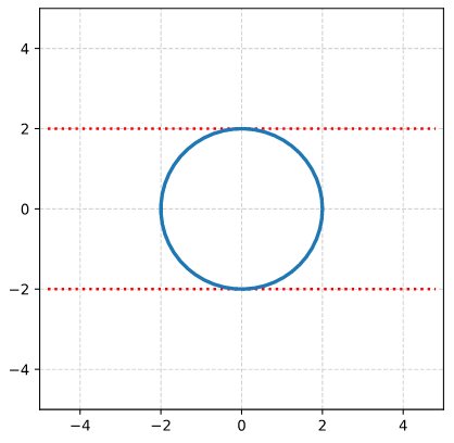
We define a circle with radius r = a = 2.
I have indicated the limiting line at the extremal y-values. From the analysis in the last post we expect that a shear operation moves the extremal points along this line.
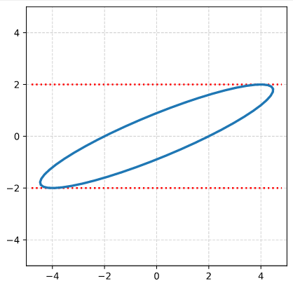
We now apply a shearing matrix with a x/y-shearing parameter λ = 2.0
Thus, we have indeed produced a rotated ellipse! We see this from the fact that the term mixing the xs and the yl coordinates does not vanish.
Position of maximum absolute y-values
We know already that the y-coordinates of the extremal points (in y-direction) are preserved. And we know that these points were located at x = 0, y = a. So, we can calculate the coordinates of the shifted point very easily:
In our case this gives us a position at (4, 2). But for getting some experience with the quadratic form let us determine it differently, namely by rewriting the above quadratic equation and by a subsequent differentiation. Quadratic supplementation gives us:
Let us also find the position of the end-points of the main axes of the ellipse. One method would be to express the ellipse in terms of the coordinates (xs, ys), calculate the squared radial distance rs of a point from the center and set the derivative with respect to xs to zero.
The “problem” with this approach is that we have to work with a lot of terms with square roots. Sometimes it is easier to just work in the original coordinates and express everything in terms of (x, y):
Plot of main axes, their end-points and of the points with maximum y-value
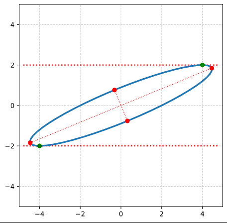
The coordinate data found above help us to plot the respective points and the axes of the produced ellipse. The diameters’ end-points are plotted in red, the points with extremal y-value in green:
It becomes very clear that the points with maximum y-values are not identical with the end-points of the ellipse’s main symmetry axes. We have to keep this in mind for a discussion of higher dimensional figures and vector distributions as multidimensional spheres, ellipsoids and multivariate normal distributions in later posts.
Rotated ECS to produce the ellipse?
The plot above makes it clear that we could have created the ellipse also by switching to an ECS rotated by the angle α. Followed by a simple scaling in x- and y-direction by the factors as and bs in the rotated ECS. This seems to be a contradiction to a previous statement in this post series, which said that a shear matrix cannot be diagonalized. We saw that in general we cannot find a rotated ECS, in which the shear transformation reduces to pure scaling along the coordinate axes. We assumed from linear algebra that we in general need a first rotation plus a scaling and afterward a second different rotation.
But the reader has already guessed it: For a fully rotation-symmetric, i.e. isotropic body any first rotation does not change the figure’s symmetry with respect to the new coordinate axes. In contrast e.g. to squares or rectangles any rotated coordinate system is as good as any other with respect to the effect of scaling. So, it is just scaling and rotating or vice versa. No second rotation required. We shall in a later post see that this holds in general for isotropically shaped bodies.
Conclusion
Enough for today. We have shown that a shear transformation applied to a circle always produces an ellipse. We were able to derive the vectors to the points with maximum y-values from the parameters of the original circle and of the shear matrix. We saw that due to the circle’s isotropy we could reduce the effect of shearing to a scaling plus one rotation or vice versa. In contrast to what we saw for a cube in the previous post.
This post requires Javascript to display formulas!
In Machine Learning samples of data vectors often undergo linear transformations. Typical examples are the adaption of vector component values due to the choice of a different shifted and/or rotated coordinate system. Another example is the scaling of vectors. As we have seen in an investigation of Autoencoders they produce multivariate normal distributions which actually are the result of linear transformations of elementary Gaussian distributions. And let us not forget that the transport between layers of neural networks includes linear transformations.
In most cases we can interpret a linear transformations in the ℝn in a geometrical way. Linear transformations are members of a sub-class of affine transformations. Affine transformations in turn can be regarded as a combination of
a translation,
a scaling in either coordinate direction,
a reflection = mirroring operation,
a rotation
and/or a shear operation.
Translations are trivial. We also understand the effects of rotation and scaling transformations intuitively. A mirror operation can be understand as a kind of inverted scaling with factors -1.
Scaling operations with different scaling factors along different coordinate directions destroy certain rotational symmetries of a 3-dimensional or n-dimensional body. But scaling transformations do not always eliminate symmetries with respect to mirroring planes: If and when we first choose an Euclidean coordinate system whose axes are aligned with symmetry axes of a body with plane symmetries, we are able to keep up at least some of the planar symmetries of the body during scaling operation.
Something that is a bit more difficult to grasp is a shear operation. The reason is that a shear operation destroys one or multiple plane symmetries of an impacted figure – whatever coordinate system we choose. And a shear operation cannot be reduced to a pure scaling operation in some cleverly chosen coordinate system. Neither can it be reduced to a rotation.
This alone is a good reason to have a closer look at this special kind of affine transformation. Another reason is to study what impact a shear operations has on the construction or transformation of a multivariate normal distribution – a topic which is at the center of another post series in this blog.
In this post I first want to discuss what a matrix that controls a shear operation looks like. We discuss some of its mathematical properties. Afterward I want to demonstrate what effects shearing has on two simple objects – a cube and a sphere. These examples will be done with Blender and the available mouse driven shear operations there.
Blender performs the required math in the background – and the examples below only provide visual impressions.
To get a better understanding of the nature of shear operation we, in the second post of this series, switch to Python and apply shear operations via explicit matrix operations onto vectors. We start with 2D-figures. Afterward we turn to 3D-cuboids and find that we produce spats. Another important example (not only with respect to multivariate normal distributions) is then given by the shearing of 3D-spheres: We will find that such an operation always produce ellipsoids. We will check this mathematically.
In a fourth post I want to discuss an important result from linear algebra, namely the so called SVD-decomposition of a linear transformation and its meaning in our context of shear operations. SVD tells us that we can always replace a shear operation by a sequence of simpler operations. We will test this statement for our 2D- and 3D-objects objects. We then also find that the creation of an ellipsoid at any orientation can be done by applying just one shear operation to a unit sphere. Alternatively, we can perform a scaling of a sphere and rotate it once. This will help us to better understand the creation of multivariate normal distributions in a parallel post series.
Shear operations break symmetries of the affected figures
A shear operation Msh introduces an asymmetry into originally symmetric figures. It does so by coupling vector components in a specific way. For reasons of simplicity we reduce our argumentation to the ℝn. We describe objects in this space with the help of position vectors to points inside and on the surface of these objects. We specify the components of position vectors with respect to an Euclidean coordinate system [ECS].
To make things easier we assume that the origin of our ECS coincides with the symmetry center of the body we apply the shear operation to. If the body has plane and point symmetries then the origin is placed at the cutting lines or the cutting point of such planes; i.e., the ECS origin coincides with the symmetry-center of the body and coordinate planes will coincide with some of the symmetry planes. For the cases we look at – spheres, cubes, coboids – the ECS origin thus gets identical with the body’s volume center.
A shear transformation applied to a vector couples at least two of the vector’s components such that a growing value for the coordinate value in the direction of a chosen coordinate axis (e.g. vz) impacts the coordinate value in another coordinate direction (e.g. vx) in a linear way.
Here is an example for the x- and z-components of a 3-dimensional vector (vx, vy, vz)T:
With α being some constant. This operation breaks an original plane symmetry of a body with respect to the x-z-plane.
A shear operation preserves the orientation of tangent planes at some surface points
But note also, that a shear operation has another unique property that keeps up a geometrical property of the affected body:
A shear operation preserves the orientation of tangent planes to the body’s surface at some particular points. The most important of these points define extrema on the surface with respect to the component whose value is linearly added in the shearing transformation. The tangent planes there do not only keep up their orientation, but also their position.
In the case defined above we would look a extrema with respect to the z-component:
\[ z \,=\, f(x,\,y), \quad { \partial f \over \partial x } \,=\, { \partial f \over \partial y } \, = \, 0
\]
Actually, we would need a bit of multivariate calculus to derive this statement for general bodies. But the example of a cube helps to grasp the central point: The transformation defined above would keep up the orientation and position of the top and the bottom square surfaces of the cube. See below for respective graphics.
In the case of a general n-dimensional body whose surface is closed, continuous and differentiable at all surface points we will find at least two such points whose tangent planes keep their orientation and position during a shearing operation.
Coupling of more than two vector components – and a restriction
Of course we could have introduced more than just one linear coupling of a selected vector component to other components. In three or n dimensions we can couple 2 components to a third one. In n dimensions we can add up shearing contributions of (n-1)-coordinate values to each of the components. But we introduce a restriction:
To avoid confusion and double shearing effects we always set αzx = 0. And analogously for the other components:
Once again: We avoid a kind of double coupling between the same pair of components. E.g., vx may become impacted by vz, but vz then shall not get impacted by vx at the same time.
Obviously, this is a an asymmetric policy in the formal handling of vector component coupling. But, it has geometrical consequences (see below). Of course, we follow this asymmetric policy also for other pairs of vector components and respective coupling parameters. This gives us a number of n*(n – 1)/2 potential constant shearing parameters.
A first example produced with the help of Blender
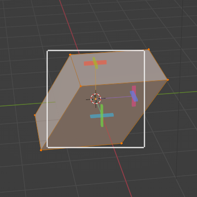
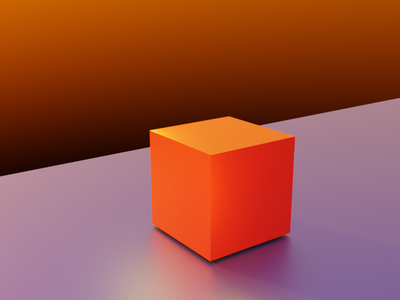
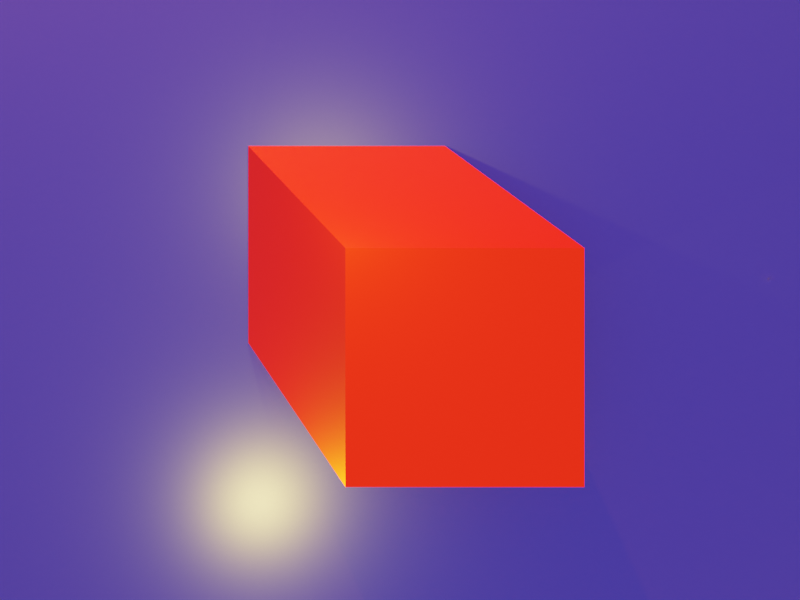
To get a visual impression of what shearing does to a body with some symmetries, let us look at a simple example: a cube.
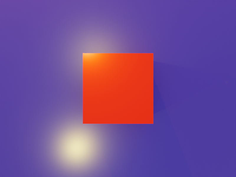
Regarding the first image we define that the x-coordinate direction goes from the left to the right, the y-direction from the front to the back and the z-direction from the bottom vertically upwards. The last image from the top shows that the x- and y-side-length of our cube are equal. Among other symmetries, a cube and also cuboids obviously have a mirror symmetry with respect to planes parallel to the x/y-plane, the y/z-plane and the x/z-plane through their centers of volume.
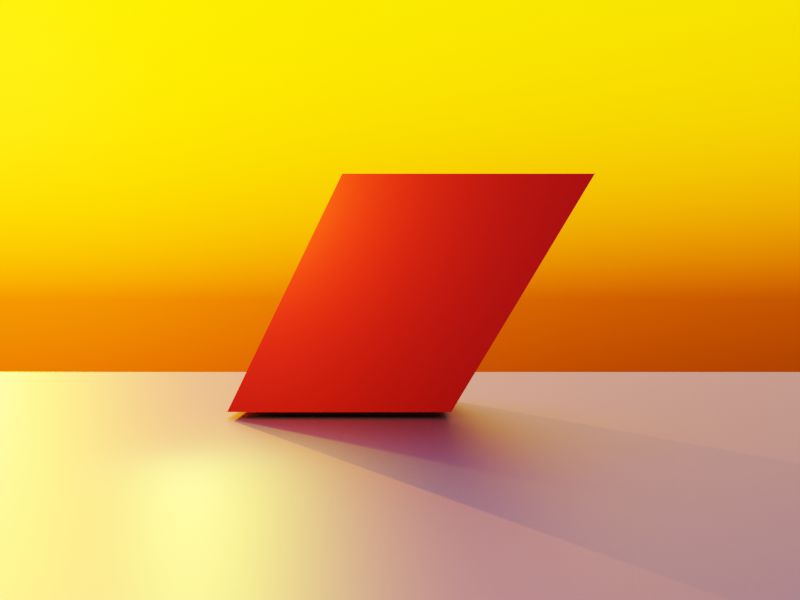
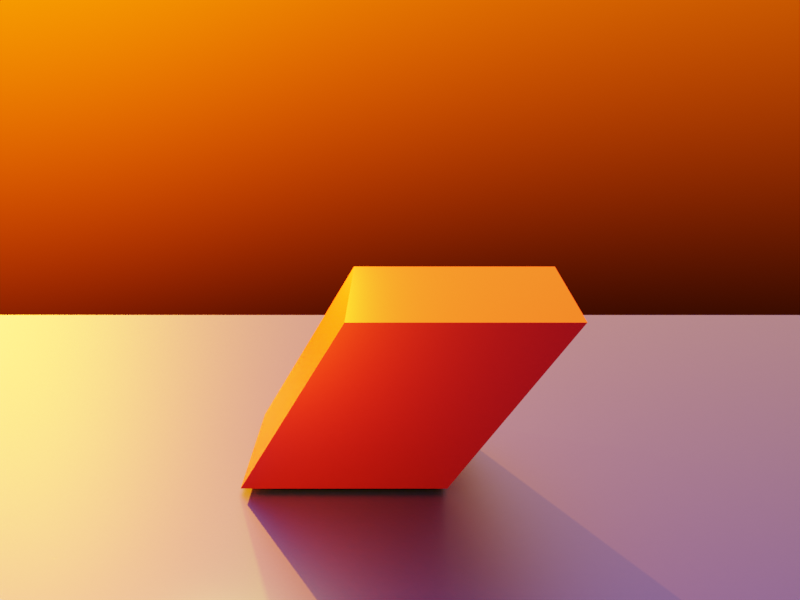
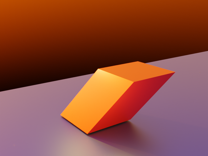
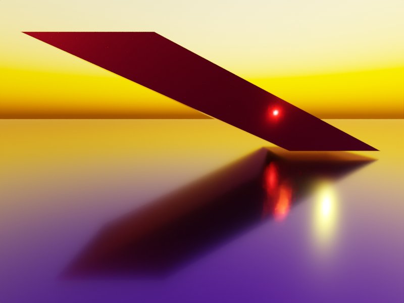
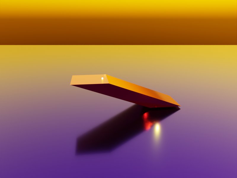
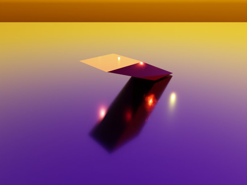
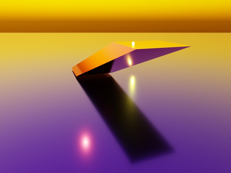
Now let us apply two shear operations which couple the x/z-coordinates and the y/z-coordinates. Then we get something like the following:
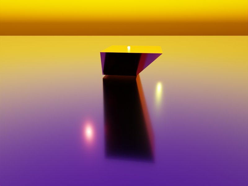
The first two image show the sheared object from the front, but with the camera moved to different heights. We see that the cube was sheared in two directions – in the x- and in the y-direction. The z-values of the upper and lower surfaces remain constant during the operation. As a result the object gets inclined in two directions: We get a spat (or parallelepiped) as the result of applying a shear operation to a cube or cuboid.
The last image shows the object from exactly the same top position as before the shearing. We see that the original symmetry is destroyed with respect to all 3 orthogonal planes (parallel to coordinate planes) through the center of volume of our object.
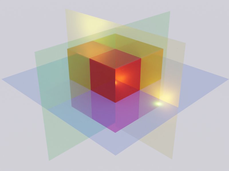
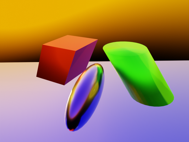
Also all of the following objects are the results of simple shearing operations. While this clear for the parallelepiped (derived from a cuboid) and the inclined cylinder (derived from a straight cylinder), it is not directly obvious for the ellipsoid which in the depicted case actually is the result of a shearing applied to a sphere (with x being impacted by y and z). In all cases rotations and translations have been applied in addition to arrange the scene.
We get the impression that some simple geometric shapes like a spat or an ellipsoid could be the direct result of one or more shearing operations applied to originally simple objects with multiple symmetries – as cubes and spheres.
Shear transformations are mathematically done by unipotent upper triangular matrices
Let us return to a more mathematical description of a shear operation. As any other linear operation applied to vectors of the ℝn we can represent a shear operation by a matrix. We just have to express the linear coupling between two vector components by a suitable arrangement of our shear-constants as matrix-elements. By experimenting a bit we find that a square matrix which only has non-zero elements on its diagonal and in its upper right triangular part does the job. We speak of an “upper triangular matrix“:
That such a matrix mixes vector components in the intended way follows directly from the definition of standard matrix multiplications. (Note: In Python/Numpy we talk about “matmul”-operations.)
Note that not all elements in the upper triangular part (aside the diagonal) are required to be different from zero. But at least one should be ≠ 0.
Not a full and neither a symmetric matrix
Now we come back to a point introduced already above: In principle we could allow for a coupling of two selected vector components in both logically possible ways. E.g., when we have an impact of the z- onto the x-component, why not also allow for an analogous impact of x- onto z at the same time? Maybe with a different linear factor?
Well, we then would get a full linear operation with possibly all n**2 elements having different values or we would get a symmetric matrices. A full generalization is not our objective. We want a special sub-case of a linear transformation. But why not allow for a symmetric matrix?
The reason for this will become clear when we discuss the decomposition and factorization of shear matrices in future posts. For the time being the following hint may help: The complexity of a linear operation can be measured by the minimum number of elementary operations required in a well chosen ECS. Can we find a coordinate system where the transformation reduces to just one elementary operation (translation, scaling, reflection, rotation)?
For a shearing transformation this would have to be a scaling operation as this kind of operation can at least potentially break rotational and planar symmetries.
Now we remember a result of linear algebra: Any symmetric matrix corresponds to an operation for wich we always can find a rotated ECS (at the center of an originally highly symmetric figure) in which the transformation of the figure reduces to a pure scaling operation.
For a shear operation we even want to exclude this kind of reduction: We shall not be able to find a ECS in which the operation just becomes a scaling. (A shearing shall in any coordinate system at least require a scaling and a rotation.) How can we achieve this? Well, we must not even allow for a symmetric matrix. For bodies which show original symmetries with respect to planes through its center this means that a shear operation destroys at least some of its planar symmetries whatever coordinate system we choose. Despite the fact that a shear operation can be inverted (see below)!
So, our elimination of some rotational and at least one planar symmetry in an originally highly symmetric body is reflected by the triangular form of the matrix. We avoid a 2-fold coupling between two selected coordinates at the same time. So when we have a matrix element mi,j, with j > i, we always set the corresponding element to zero: mj,i = 0.
This restricts the distortions we are going to get. Some surface elements are going to remain congruent and some point symmetries are kept up.
Why did we not use a lower triangular matrix?
Well, this is just a convention. Actually, the transposed matrix of an upper triangular one would also do the job – so we could also take matrices with non-zero elements only in the lower left triangle. But, for convenience, we will stick to matrices with non-zero elements in the upper right triangular part.
What about the diagonal elements of a shear matrix?
First of all note that not all elements on the diagonal of the matrix Msh should become zero – because then we would eliminate our original figure totally. But for a shear operation we do not want any of the vector components to disappear! In addition: As non-zero elements in the diagonal would reflect a simple scaling we do request that all of the diagonal matrix elements should be equal to 1 for a pure shear operation:
As the diagonal is fixed by elements mi,i(>i) = 1, we have reduced the number of free and independent (off-diagonal) parameters Nindsh(>i) of a pure shear matrix Msh from n**2 to:
So, in 2 dimensions instead of 4 parameters we set the diagonal elements to 1 and choose just 1 free off-diagonal parameter. In 3 dimensions we only have to set 3 instead of 6 off-diagonal parameters.
Basic properties of a shear matrix
A quick calculation shows: The determinant of a shear matrix is directly given by the product of its diagonal elements, and thus we have:
Therefore, a shear matrix is always invertible. This means its effects can be reverted – also in geometrical terms. The matrix also has full rank r = n.
The eigenspace and the eigenvalue(s) of a shear matrix Msh are also interesting. We can use a property of triangular matrices to get the eigenvalue(s):
The diagonal elements of a triangular matrix are its eigenvalues.
This in turn can be understood from analyzing the characteristic polynomial det(M – λI) = 0.
Thus: The one and only eigenvalue ev of Msh is 1.
\[ \pmb{ev}_{\operatorname{M}_{sh}} \, = \, 1
\]
The eigenvalues algebraic multiplicity in the characteristic polynom is n This does not yet tell us much about the geometrical multiplicity, i.e. the dimension of the eigenspace.
But all the n eigenvalues share the same eigenspace ES. ES is the kernel of the matrix (A – λI). Therefore, we can derive the eigenspace’s dimension by the dimension formula for this particular matri:
as the rank of the combined matrix on the right side is (n – 1).
You also see this understand this by looking at the 4-dim example matrix given above:
When you write down the equations you will find that only 1 variable can be chosen freely. So the kernel of the matrix (A – λI) is only 1-dimensional. Logically and geometrically, this is clear as any other coordinate value (≠ 0) beyond the first one mixes in contributions.
It is easy to prove that the eigenspace ES can be based upon the eigenvector e1.
Can Msh be diagonalized? Answer: No! From linear algebra we know that this would require n linearly independent eigenvectors. But we have just one! So:
Think a bit about the consequences:
An operation like that on the right side of the un-equation above would correspond to the representation of our shear matrix in a different (rotated) coordinate system. A diagonalization corresponds to an eigendecomposition; in geometrical terms a diagonal matrix represents a pure scaling operation. But, obviously, such a description of our shear operation in some (cleverly) selected ECS is not possible:
We cannot find a (translated and rotated) ECS in which a shear operation reduces to a scaling transformation. In any chosen (rotated) ECS there is always an additional second rotation involved which we cannot simply invert or get rid off!
We shall see this in more detail when we discuss decompositions. We simply cannot get rid of the fundamental asymmetry we have build into Msh by not allowing non-zero elements in the lower triangular part of the matrix! No change to a whatever selected coordinate system will help.
So, a shear operation really is a special symmetry breaking operation which cannot be reduced to just one elementary operation. In any ECS it requires at least a rotation and a scaling!
Summary:
A pure shear operation is introduced by some off-diagonal and non-zero element in the upper right triangular part of a unipotent matrix. All off-diagonal elements in the lower left triangular part are set to zero.
More illustrations from Blender
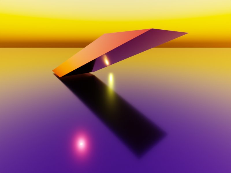
First some images for a cuboid that was more extremely deformed by shearing in x- and y-direction than the first one:
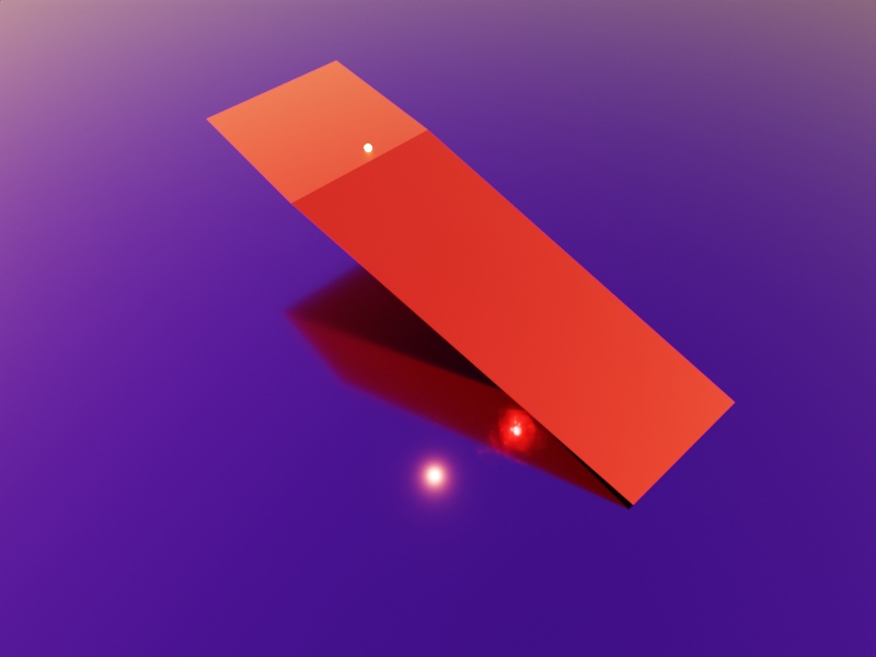
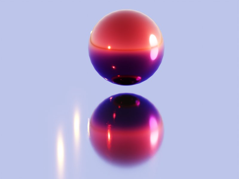
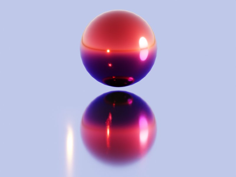
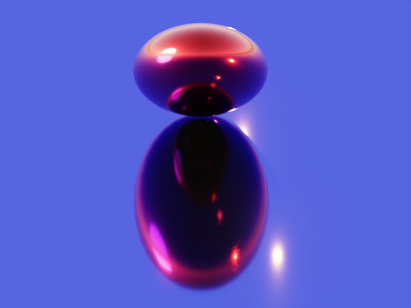
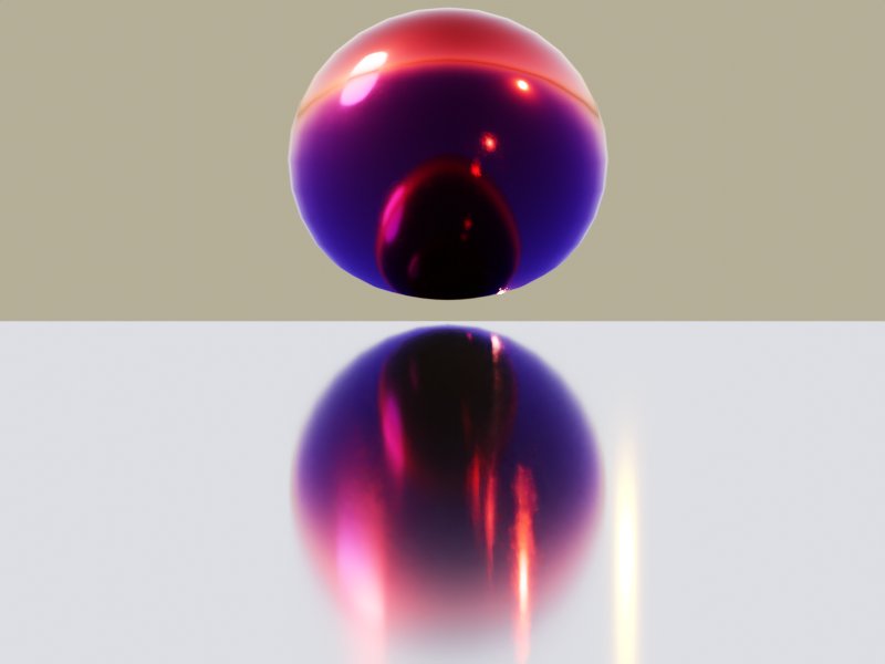
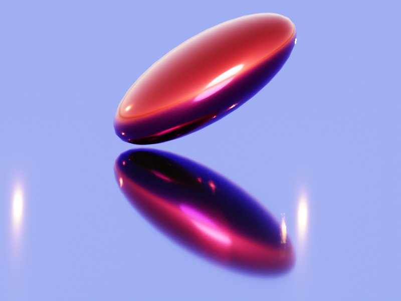
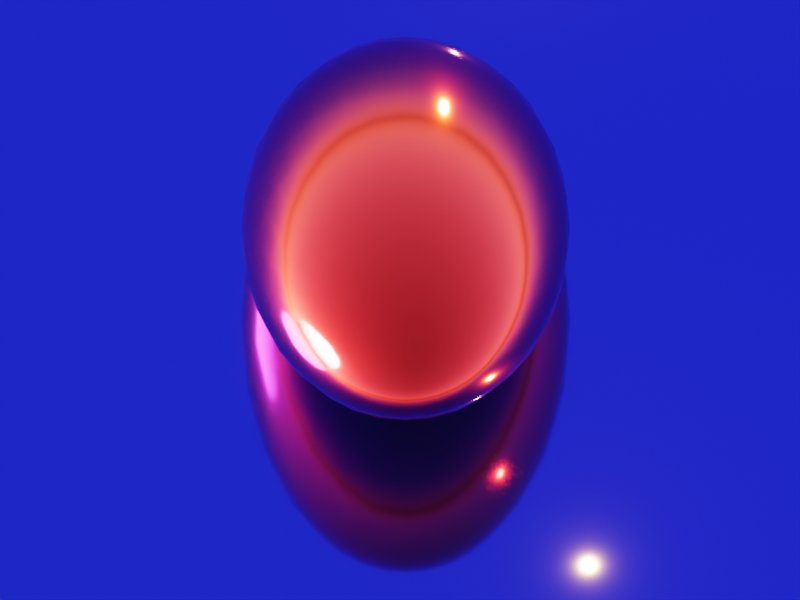
Now we come to an interesting example: We apply shearing in x- and y-direction to a sphere. We get something whose shape looks much more regular than that of a cuboid. We pick a unit sphere and apply to shearing operations in x- and y-direction:
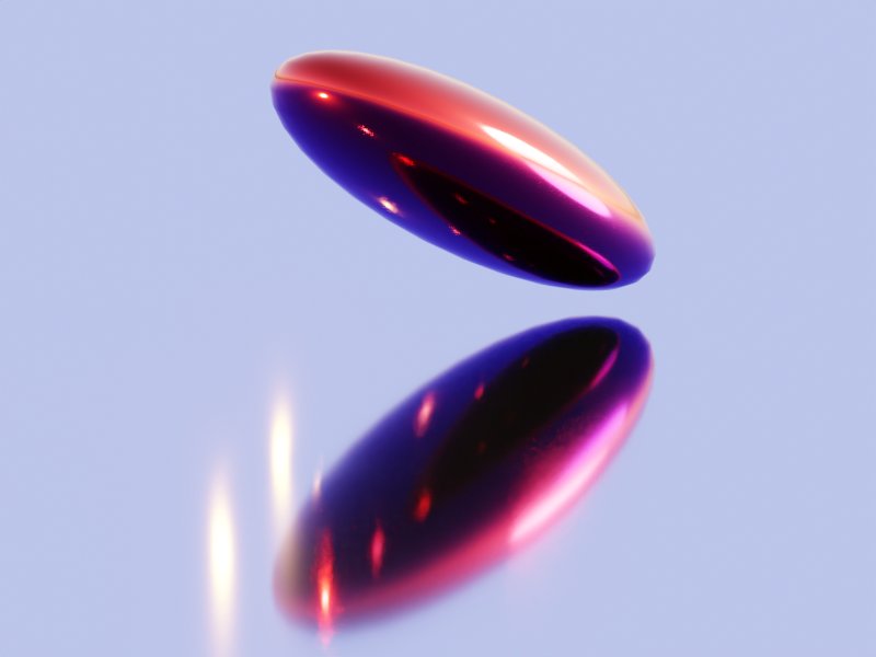
The first image shows the original sphere from some point of view. The second image was taken from the same perspective, but now after the shearing. The resulting figure looks very regular – and it seems to have plane symmetries.
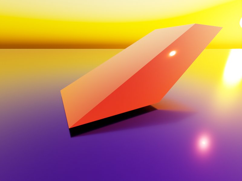
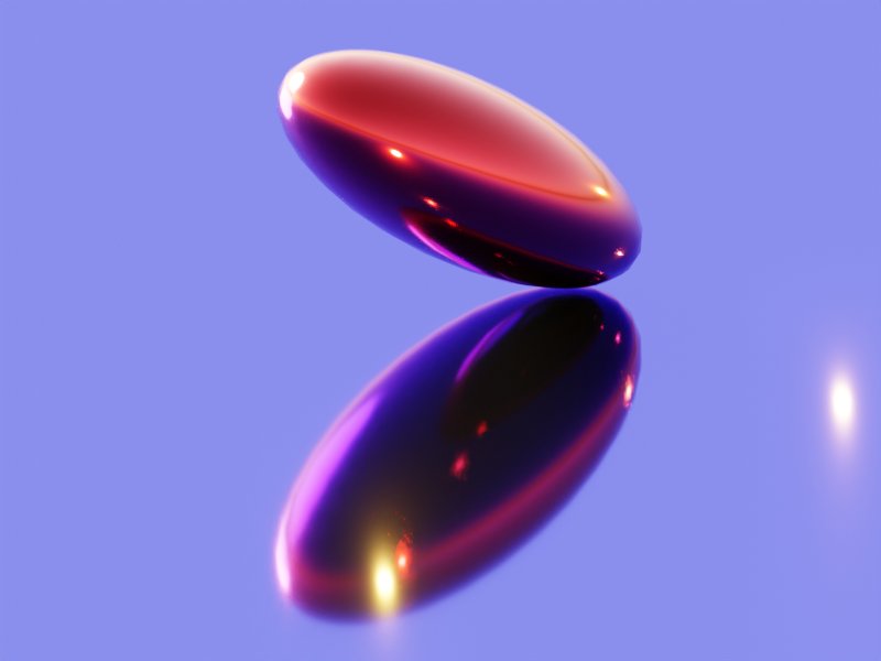
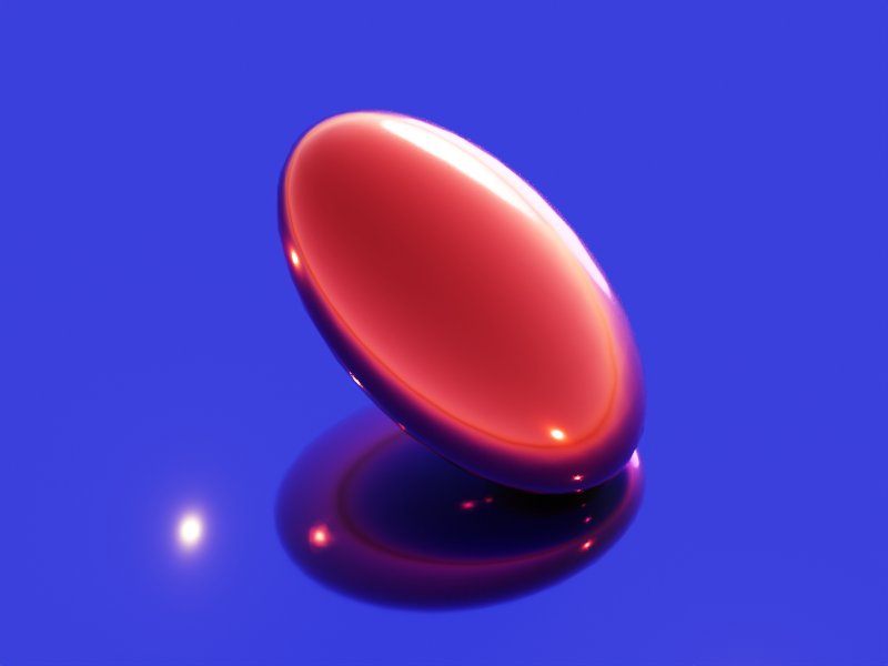
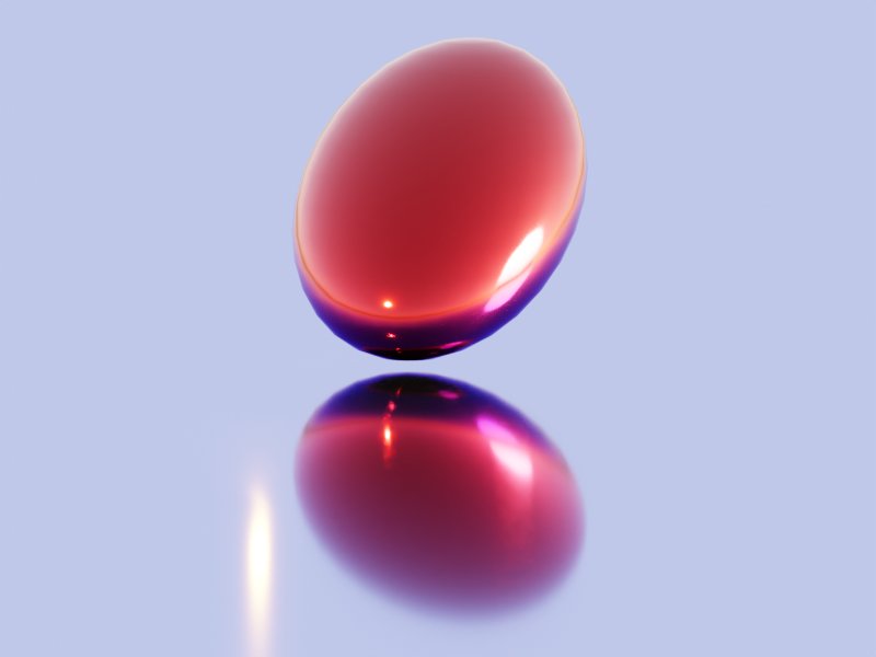
Another example with a bit of different lighting gives us:
Actually, we get an ellipsoid. We clearly can identify the two points which have a maximum absolute z-values whose tangent planes did not change tier orientation.
Ellipsoids (in 3D) are figures with 3 main axes and planar symmetries. The original fully rotational symmetry (first image of the series above) is obviously broken. However, we seem to have saved at least some planar symmetries. Hmmm …. Just when we thought we had understood that a shearing operation breaks original planar symmetries we have in our new example case kept some.
Why is this? What is so special about the shearing of spheres? Keep this question in mind.
Conclusion
Shearing transformations are a special class of linear and thus transformations. Shearing obviously can break some plane symmetries of originally highly symmetric bodies – as cubes. In contrast to other elementary affine operations no coordinate system can be found where the number of operations to reproduce the effects of a shearing can be reduced to one. In particular it is not possible to find an Euclidean coordinate system where it is just reduced to a (symmetry breaking) scaling with different factors in different coordinate directions.
Blender offers a simple graphical method to apply shearing to simple geometrical bodies. This allowed us to get an impression of the effects on cubes and spheres. Something that was a bit astonishing was the shearing effect on a unit spheres. It just created ellipsoids – again highly symmetric bodies WITH planar symmetries.