
This post requires Javascript to display formulas!
This post series is about shear transformations and related matrices.
In the end we want to better understand the effect of shear operations on “multivariate standard normal distributions” [MSND]. A characteristic property of a MNSD is that its contour hyper-surfaces of constant density are nested spheres. We want to understand the impact of a shear operation on such a random vector distribution.
In the first post of this series
Fun with shear operations and SVD – I – shear matrices and examples created with Blender
we have already had a preliminary look on shear transformations. We have seen that shear transformations are a special class of affine transformations. They are represented by square unipotent, upper (or lower) triangular matrices. The eigenspace is 1-dimensional and the only eigenvalue is 1.
We have also understood that a shear operation can not be reduced to a simple scaling operation with different factors by choosing some special rotated Euclidean coordinate system [ECS], whose origin coincides with volume and symmetry center of the original figure.
Due to its matrix properties which are very different from orthogonal matrices a shear operation is neither a rotation, nor a scaling. Instead we suspect that it might only be decomposed into a combination of a rotation plus a scaling – whatever coordinate system we choose. We still have to prove this in a forthcoming post.
In this post we want to explicitly apply shear matrices to simple 2D- and 3D-figures, namely squares and cubes. We use Python to control the operations and visualize the results with the help of Matplotlib. We will check that the position and orientation of all extremal points in y-direction (2D-case) and z-direction (3D-case) are preserved during shearing. We will depict this by applying the transformations to position-vectors, which point to elements of distinct vertical layers. In 3D I also test the effects of shearing on cubes by just using the 8 corner points of the cube to define 6 faces, which then get transformed.
Afterward we briefly look at the chaining of shear operations and the resulting product of their respective matrices. As some people may think that one could use combinations of shears induced by a mix of upper triagonal and lower triagonal matrices, we investigate the effects of such combinations. We see that such combinations hurt conditions we have already defined for pure shear operations. Even a symmetric matrix, which has the same shear factors in the upper and lower triangular parts of the matrix has a different effect than a real shearing: It distorts a body in the sense of a pure scaling with different factors in potentially all orthogonal directions.
Hint: I omit Python code in this post. If I find the time I will deliver some code snippets at the end of this post series. However, it is really easy to set up your own programs to reproduce the results of my experiments and respective plots with the help of Numpy and Matplotlib.
Before showing results of numerical experiments I first list up some general affine properties and other specific properties of shear transformations.
Affine properties of shear transformations
Important properties of all affine transformations are:
- Collinearity: points on a line are transformed into points on a line.
- Parallelism: Parallel lines remain parallel lines. Lines remain lines. Planes are transformed into planes.
- Preservation of sub-dimensionality: Affine transformations preserve the dimensionality of objects confined to a sub-space of the “affine” space they operate on.
- Convexity: Convex figures remain convex – i.e. the sign of a curvature radius does not change.
- Proportionality: Distance ratios on parallel line segments are preserved.
Extremal points on convex surfaces may remain extremal with respect to distances to the origin, but not with respect to a specific coordinate axis (rotation!). Note that the third point holds for convex (hyper-) surfaces – as e.g. that of a sphere or ellipsoid.
Properties of shear transformations and their matrices Msh
I list some properties which I have already discussed in my previous post:
- Fix point: When we omit a translation it is natural to choose an Euclidean coordinate system [ECS] such, that its origin coincides with the symmetry center of the body to be sheared. This point then remains a fixed point of the transformation.
- Msh is a unipotent matrix with non-zero-elements only in its upper (or lower) triangular part. The matrix elements on the diagonal are just 1.
- det(Msh) = 1. A shear transformation is invertible. Its rank is rank(Msh) = n.
- The only eigenvalue ε is ε = 1. Its multiplicity in the ℝn is n.
- The eigenspace ESsh has a dimension dim(ESsh) = 1.
- A single pure shear mediated by a unipotent upper (or lower) matrix can not be reduced to a pure scaling operation in some cleverly chosen, rotated coordinate system.
For reasons of convenience we below again chose an Euclidean coordinate system [ECS] whose origin coincides with the center of volume or the symmetry center of a body which we apply a shear transformation to. This not only guarantees a central fixed point. The structure of the diagonal matrix and the 1s on the diagonal
\begin{pmatrix}
1 & m_{12} &\cdots & m_{1n} \\
0 & 1 &\cdots & m_{2n} \\
\vdots &\vdots &\ddots &\vdots \\
0 & 0 &\cdots & 1 \end{pmatrix}, \\
\pmb{v}^{sh} \: &= \: \pmb{\operatorname{M}}_{sh} \circ \pmb{v} \phantom{\Huge{(}}
\end{align}
\]
make it clear that the last component of any affected vector remains constant during a shear transformation:
\begin{align}
\pmb{v} \: &= \: (\, v_1, \, v_2, \,\cdots \, v_n)^T, \\
\pmb{v}^{sh} \: &= \: (\, v_1^{sh}, \, v_2^{sh}, \,\cdots \, v_n^{sh})^T \phantom{\huge{(}} \\
v^{sh}_n \: &= \: 1.0 \, *\, v_n \phantom{\huge{(}}
\end{align}
\]
This is independent of the linear coupling between other components. Therefore, an important feature of a shear operation is:
Extremal points on the surface of a sheared body in the n-th coordinate direction remain extremal and are moved within a hyper-plane orthogonal to the sub-space ℝ1 of the ℝn.
And, more generally:
Points of a sheared body lying in a (n-1)-dimensional sub-space of the ℝn, which are defined by vn = const, are moved within the sub-space, only, during shearing.
In 3D with coordinates (x, y, z) such a sub-space is a hyper-plane defined by z = const.. E.g. for a cube the points of the top face in z-direction are elements who just move within this plane during a shearing-operation. The same holds for any layer of points defined by other values z = const. Actually, the extremal points in z-direction even move along defined straight lines within the plane. In the general case these lines cross the (n-1)-dimensional sub-space.
It is time to take Python to perform some numerical experiments in 2D and 3D – and visualize the above statements. As said, in this post we concentrate on the shearing of squares and cubes. And the behavior of extremal points and other points located on layers with a constant value of the preserved vector component. I admit that squares and cubes are a bit boring, but this post is just a preparational step towards a closer investigation of the the impact of shear operations on statistical vector distributions controlled by Gaussians.
2D: Shearing of a square/rectangle
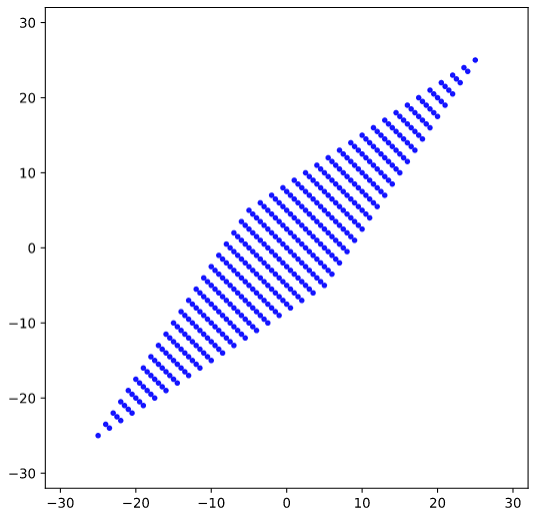
The figure below shows the end-points of position-vectors, which define data points on a rectangular meshes within a square. All the points reside inside and on the boundary of the square and reflect horizontal layers of the square:
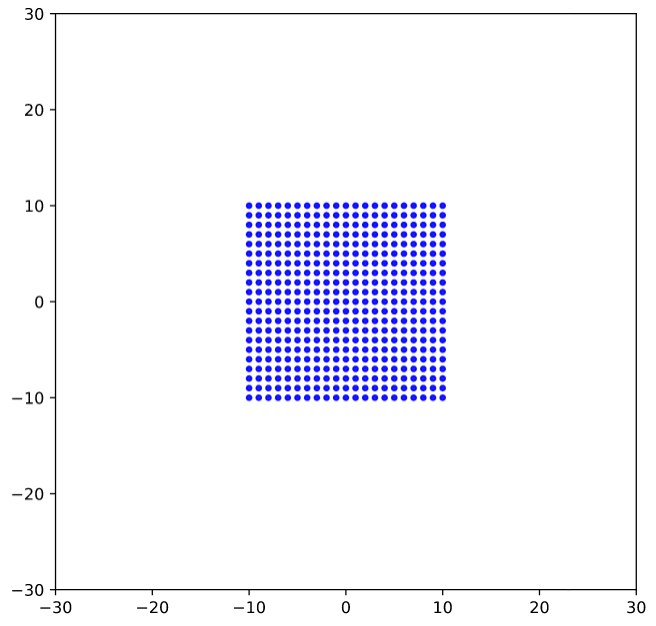
Now we apply a shear matrix with the following elements [[1.0, 1.5], [0.0, 1.0]]. As we only work in two dimensions our matrix just has 4 elements with values ≠ 0. We name the undisturbed vectors of our square vsq. The resulting vectors after the shear operation will be called vsh. I.e.:
\]
and
\]
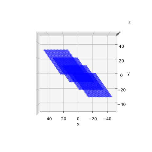
A plot of all the vsh gives us:
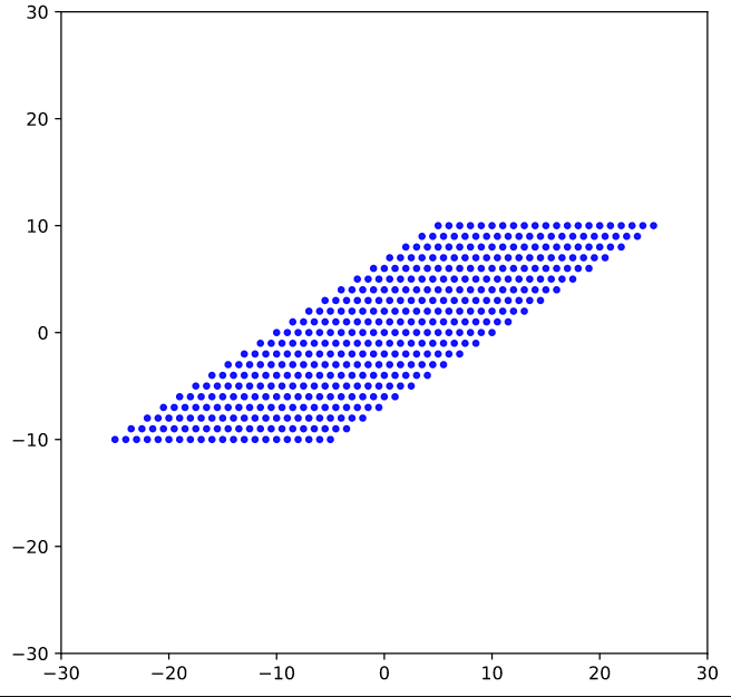
Exactly, what we expected. We directly see the constant shift of layers against each other. And we also see the linearity of the overall effect in the diagonal lines between the new edges. The overall result is a parallelogram.
The points on all the layers were moved along hyper-surfaces with y = const., which in our 2D case are just lines parallel to the x-axis.
Note that the symmetry center at the origin of our figure remained fixed. Point symmetries with respect to the original symmetry center have been preserved. However, original symmetries with respect to the coordinate axes have been broken.
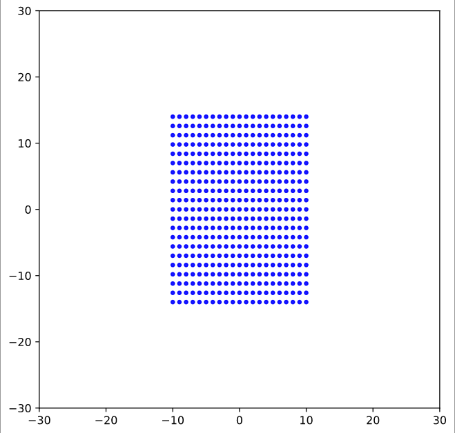
For a rectangle we get analogous, stretched images:
Shear transformation of a cube
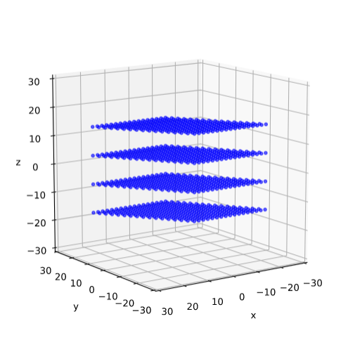
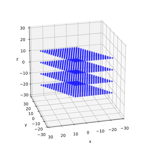
The last plots were simple, but visualized the very nature of a shear transformation: Linear differences of (position) vectors between layers. Breaking of plane symmetries for polytopes, while point symmetries are preserved. Let us try to demonstrate something similar in 3D. Once again an illustrative method to do this is to produce multiple planes on different z-levels filled with points on a regular mesh. During plotting we allow for some transparency of these points.
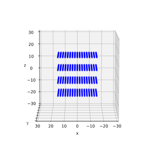
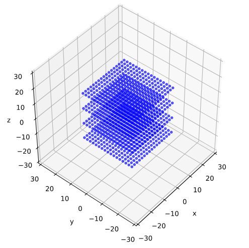
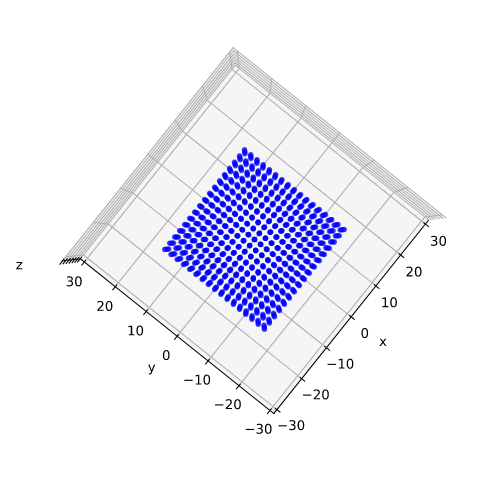
All images show the situation before shearing. You see the flat squares (extending in x- and y-direction) on 4 different z-levels. It can be seen that the dimensions are -15 ≤ vi ≤ 15, for i ∈ {1, 2, 3}. We now apply a shear matrix Msh = [[1.0, 0.7, 0.0], [0.0, 1.0, 0.0], [0.0, 0.0, 1.0]]
\\ 0.0 & 1.0 & 0.0 \\
0.0 & 0.0 & 1.0
\end{pmatrix}
\]
to the position-vectors of our layer points. I.e. we only induce a linear effect of the y-components onto the x-components of our vectors. The result is:
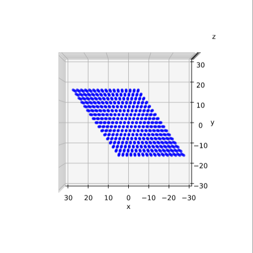
We get a systematic y-dependent change of the x-coordinate values of our points. The z-level of our layer points, however, remain unchanged. Now, we repeat our experiment, but this time we add an additional shear via a linear dependency of x- and y-component values of our vectors on their z-component by
\\ 0.0 & 1.0 & 1.0 \\
0.0 & 0.0 & 1.0
\end{pmatrix}
\]
The shift of the layers against each other in x- and y-direction gets a clearly visible z-dependence:
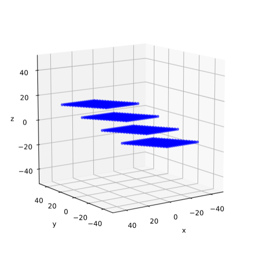
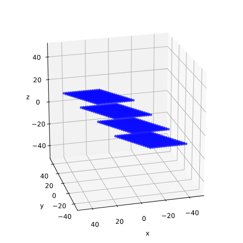
But, again and of course, all elements of our 4 layers remain on their respective z-level.
Shearing of a cube: Surface layers
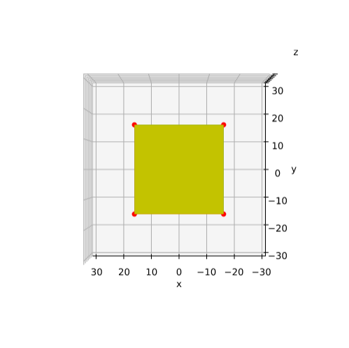
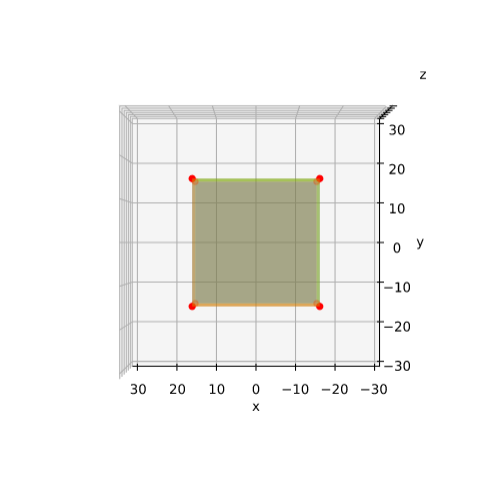
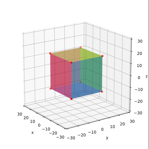
An alternative method to visualize the impact of a shear-transformation on a cube with the help of Matplotlib is based on 8 vectors that span the 6 surface elements of the cube. We also make the cube-faces a bit transparent in some plots. The original cube then looks like:
The result for our last shear matrix
\\ 0.0 & 1.0 & 1.0 \\
0.0 & 0.0 & 1.0
\end{pmatrix}
\]
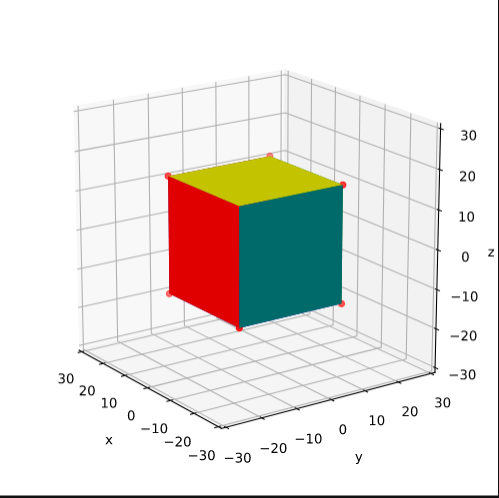
is:
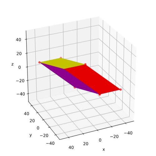
Here wee see again that the z-level of the upper and lower limiting plates of the cube remained constant. They were just moved in x- and y-direction:
Our shear operation has produced a parallelepiped or a spat. This is consistent to the results of Blender experiments depicted in my previous post.
Remarks on a significant deficit of Matplotlib for 3D
A significant problem that one stumbles into with plots like those above is that Matplotlib does not offer us a real 3D engine. Meaning: It often calculates the so called z-order of objects like hyper-planes (or parts of such), curved manifolds, bodies along our fictitious line of visibility wrongly. So, the shading of e.g. transparent and opaque surfaces according to overlaps in 3D along your line of sight is almost always depicted in a wrong way.
For complex bodies this can drive you crazy and makes you wonder if it would be better to learn controlling Blender with Python. For our relatively simple cases I solved the z-order problem by disabling the computed z-order
ax = fig.add_subplot(111, projection=’3d’, computed_zorder=False)
and by manually assigning a z-order-value to each of the cube’s faces.
Still: As soon as we distort a simple body as a cube strongly (see below) you need a really good overview about the order of your surfaces and their colors after rotations. It is worthwhile to make sketches or to create a similar body with Blender first to clearly see, what happens during a sequence of rotations.
Combinations of shear transformations
Shearing transformations can, of course, be chained in an orderly sequence of operations. Let us take a 2D example of two shear matrices with the same shear-parameter:
\begin{pmatrix} 1 & \lambda \\ 0 & 1 \end{pmatrix} \circ
\begin{pmatrix} 1 & \lambda \\ 0 & 1 \end{pmatrix}
\\
&= \: \begin{pmatrix} 1 & 2\lambda \\ 0 & 1 \end{pmatrix} \phantom{\Huge{(}^T}
\end{align}
\]
For different shear parameters we get
\begin{pmatrix} 1 & \lambda \\ 0 & 1 \end{pmatrix} \circ
\begin{pmatrix} 1 & \mu \\ 0 & 1 \end{pmatrix}
\\
&= \: \begin{pmatrix} 1 & \lambda \, +\, \mu \\ 0 & 1 \end{pmatrix} \phantom{\Huge{(}^T}
\end{align}
\]
I.e., we just increase the shearing effect by performing two shear operations after another. If we had taken the negative value (μ = – λ) we would just have inverted the shearing. Note:
A chaining of pure shear matrices, which we had defined as upper triangular matrices in the first post, is a symmetric operation with respect to the order of the matrices.
Combination of upper and lower triangular shear matrices?
However, what happens if we combine an unipotent upper triangular shear matrix with a lower triangular matrix with the same shearing coefficient?
\begin{pmatrix} 1 & \lambda \\ 0 & 1 \end{pmatrix} \circ
\begin{pmatrix} 1 & 0 \\ \lambda & 1 \end{pmatrix}
\\
&= \: \begin{pmatrix} 1 \,+\, \lambda^2 & \lambda \\ \lambda & 1 \end{pmatrix} \phantom{\Huge{(}^T}
\end{align}
\]
We get a symmetric matrix. This is not surprising, as this always is the case for product of a matrix with its transposed counterpart. But, in addition, a scaling is superimposed. Note also that the combined operation is not symmetric regarding the order of matrix application:
\begin{pmatrix} 1 & 0 \\ \lambda & 1 \end{pmatrix} \circ
\begin{pmatrix} 1 & \lambda \\ 0 & 1 \end{pmatrix}
\\
&= \: \begin{pmatrix} 1 & \lambda \\ \lambda & 1 \,+\, \lambda^2 \end{pmatrix} \phantom{\Huge{(}^T}
\end{align}
\]
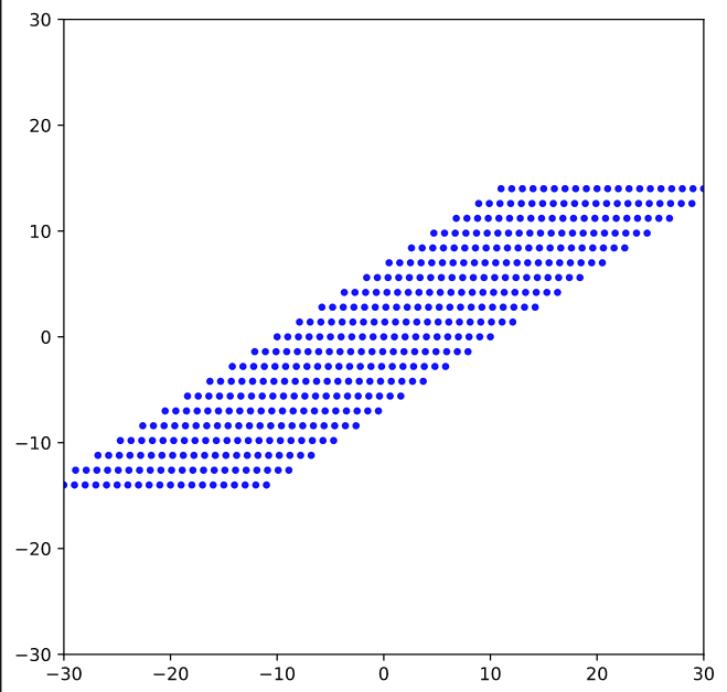
Let us apply the second variant to our square (see above) for λ = 1.5:
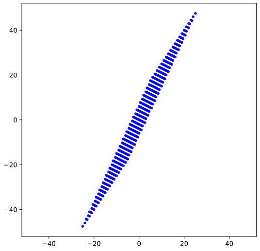
As expected we get a stronger distortion in y-direction. Note also that in contrast to a normal shear operation z-levels of our 4 level-rows were not preserved. Instead the individual levels appear rotated and stretched. Actually, in one of the next posts we will see that our combined matrix can be factorized into a combination of a rotation, then pure scaling, then back-rotation (by the same angle used in the first rotation). But this corresponds to nothing else than a pure scaling in a rotated ECS.
The funny thing with chaining is that using a simple symmetric matrix from the start for λ = 1.5
\begin{pmatrix} 1 & \lambda \\ \lambda & 1 \end{pmatrix}
\]
would give us a different result than a sequence of MshT * Msh:
Note:
Combining a shear matrix with its transposed is something different than just using a matrix with filling in (transposed) elements in the lower part with the same value as their mirrored elements in the upper triangular part.
By combining upper and lower triangular shear matrices we leave the group of pure shear operations
We could call the application of a symmetric matrix a kind of symmetric shearing. But even with a symmetric matrix we loose the central property of a normal shear operation, namely that the z-levels of body-layers parallel to the x/y-plane are preserved. All in all we get into trouble as soon as we combine original shear matrices and their transposed counterparts. Regarding my definition of a shear matrix in my previous post, we obviously leave the group of shear operations by such a combination. Some reader may regard this as an exaggeration. But it makes sense:
Even the symmetric matrix of the combined operation can be reduced to a pure scaling operation in a rotated coordinate system. And this simply is not shearing.
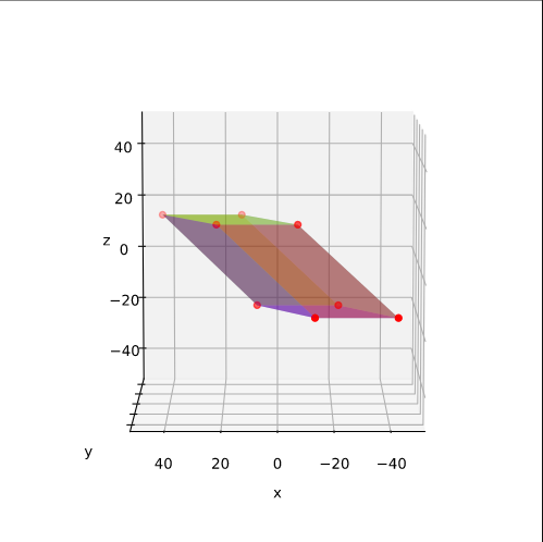
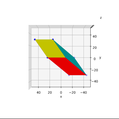
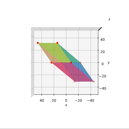
Just for fun: “Symmetric shearing” applied to a cube
Just for the fun of it, let us apply a symmetric version of a 3D-shearing matrix to our cube:
shear = [[1.0, 0.6, 1.0], [0.6, 1.0, 1.2], [1.0, 1.2, 1.0]]
1.0 & 0.6 & 1.0 \\
0.6 & 1.0 & 1.2 \\
1.0 & 1.2 & 1.0
\end{pmatrix}
\]
We expect all layers to be stretched into all coordinate directions now; z-levels of the original layers parallel to the x/y-plane will not be preserved. The normal vector to the transformed layers will be inclined to all axes after the operation.
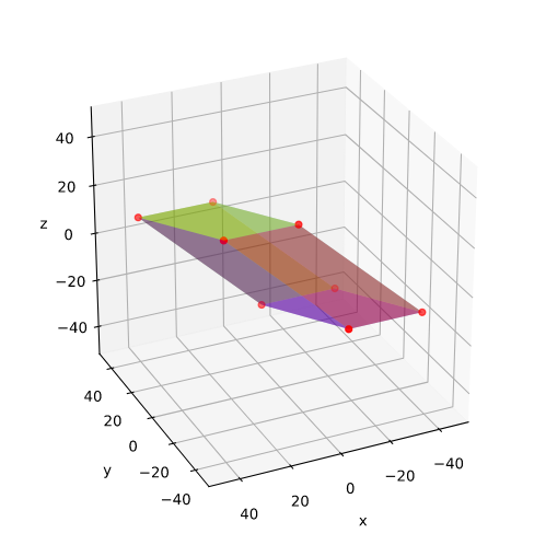
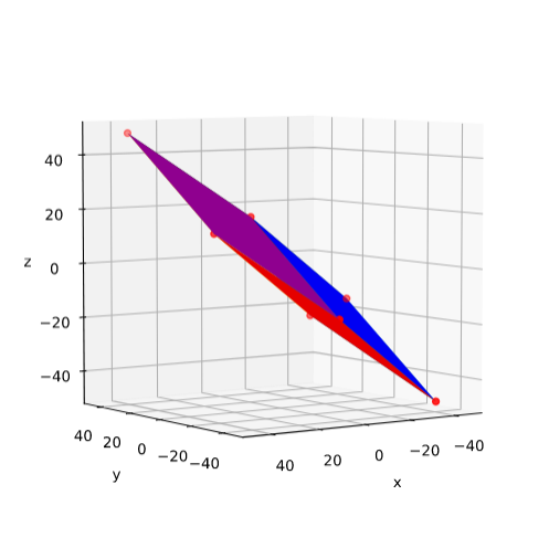
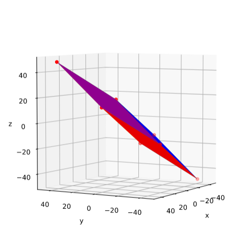
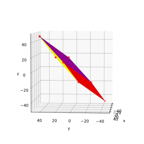
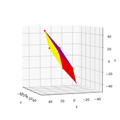
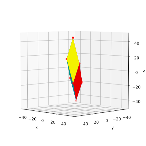
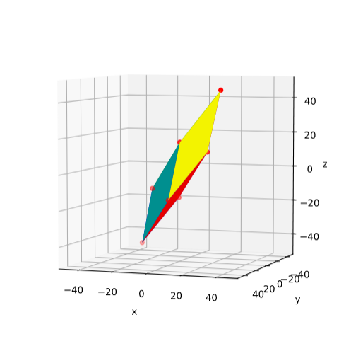
The following plots were done with intransparent, opaque surfaces. Due to the extreme stretching we would otherwise loose the overview – which is nevertheless difficult. I have kept the order of colors for the cubes side-layers the same as for the unstretched cube: sf_color=[‘yellow’, ‘blue’, ‘red’, ‘green’, ‘magenta’, ‘cyan’]. I first give you some selected perspectives:
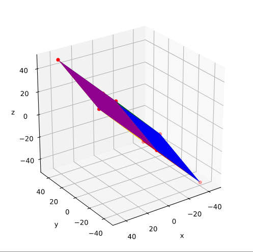
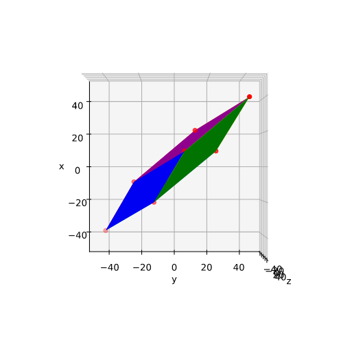
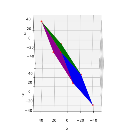
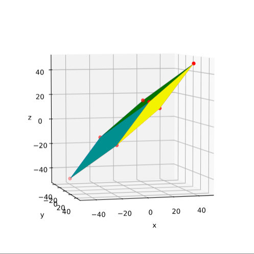
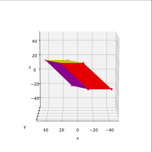
The distortion in all directions is obvious. Note that the point-symmetries of all corners with respect to the origin are preserved. The following sequence reflects views from a circle around the vertical axis:
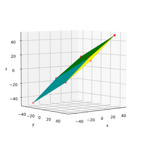
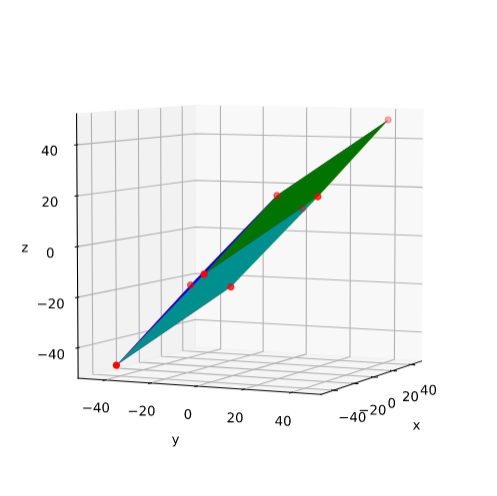
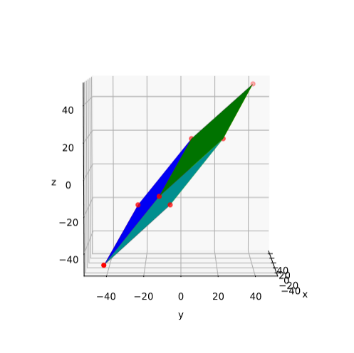
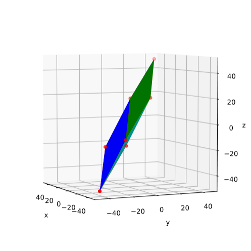
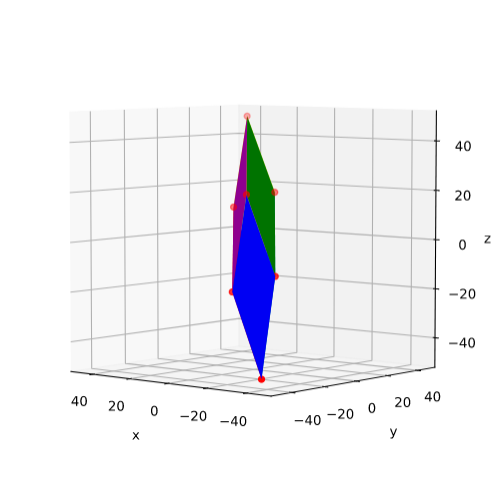
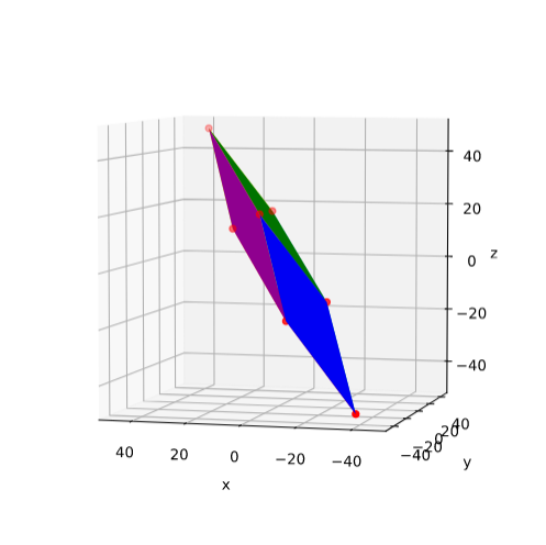
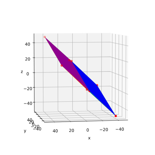
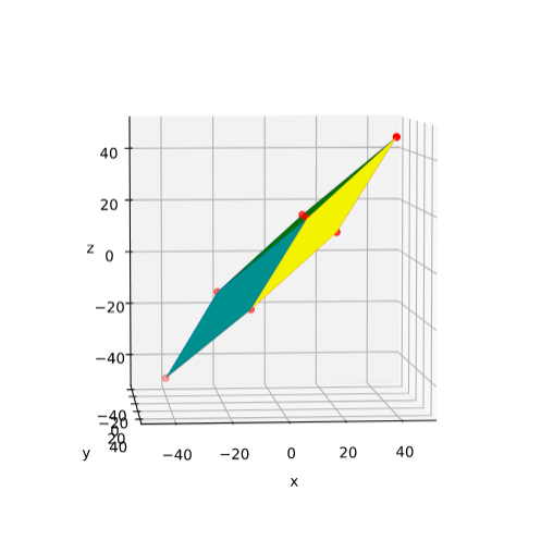
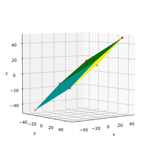
What we learn is that even scaling alone can distort a symmetric body quite a lot.
Conclusion
In this post I have visualized the effect of shear operations on squares and cubes. We saw that working with points on layers and with respective vectors is helpful when we want to demonstrate a central property of real shear operations: One vector component stays as it is. Nevertheless, the symmetry breaking of shearing transformations was clearly visible. We also saw that we should represent shear transformations either by upper or lower triangular matrices, but we should not mix these types of matrices.
As a side effect we have seen that a combination of shear matrix with its transposed induces strong deformations in specific coordinate directions by enhanced scaling factors. Symmetric matrices also lead to relativ strong distortions. We have claimed that these distortions can be explained by pure scaling operations in a rotated coordinate system. A proof has to be delivered yet.
In the next post
Fun with shear operations and SVD – III – Shearing of circles
we take a first step in the direction of shearing multivariate normal vector distributions. We keep it simple and just study the impact of shearing transformations on circles.