In the first three articles of this series on a (very) simple CNN for the MNIST dataset
A simple CNN for the MNIST dataset – III – inclusion of a learning-rate scheduler, momentum and a L2-regularizer
A simple CNN for the MNIST datasets – II – building the CNN with Keras and a first test
A simple CNN for the MNIST datasets – I – CNN basics
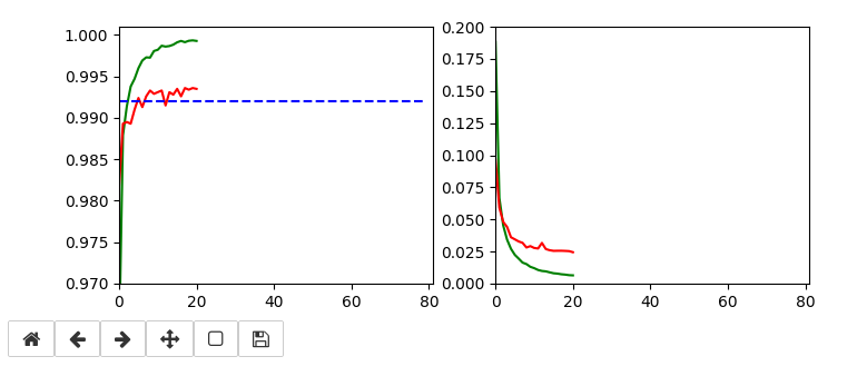
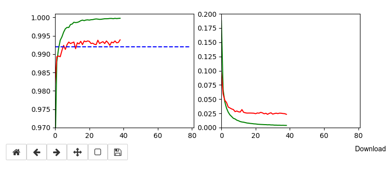
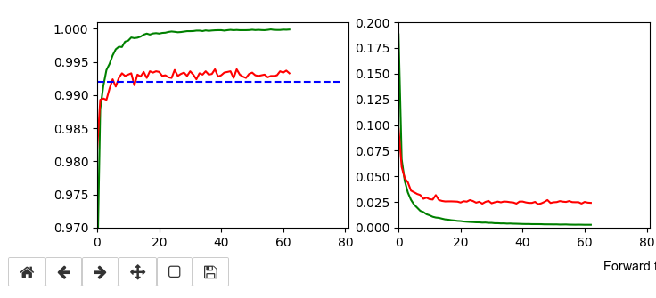
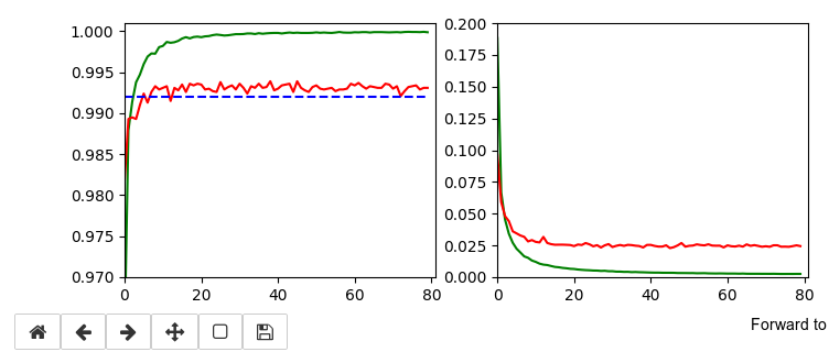
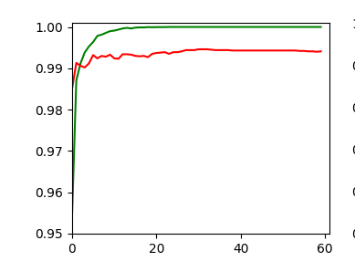
we invested some work into building layers and into the parameterization of a training run. Our rewards comprised a high accuracy value of around 99.35% and watching interactive plots during training.
But a CNN offers much more information which is worth and instructive to look at. In the first article I have talked a bit about feature detection happening via the “convolution” of filters with the original image data or the data produced at feature maps of previous layers. What if we could see what different filters do to the underlying data? Can we have a look at the output selected “feature maps” produce for a specific input image?
Yes, we can. And it is intriguing! The objective of this article is to plot images of the feature map output at a chosen convolutional or pooling layer of our CNN. This is accompanied by the hope to better understand the concept of abstract features extracted from an input image.
I follow an original idea published by F. Chollet (in his book “Deep Learning mit Python und Keras”, mitp Verlag) and adapt it to the code discussed in the previous articles.
Referring to inputs and outputs of models and layers
So far we have dealt with a complete CNN with a multitude of layers that produce intermediate tensors and a “one-hot”-encoded output to indicate the prediction for a hand-written digit represented by a MNIST image. The CNN itself was handled by Keras in form of a sequential model of defined convolutional and pooling layers plus layers of a multi-layer perceptron [MLP]. By the definition of such a “model” Keras does all the work required for forward and backward propagation steps in the background. After training we can “predict” the outcome for any new digit image which we feed into the CNN: We just have to fetch the data form th eoutput layer (at the end of the MLP) after a forward propagation with the weights optimized during training.
But now, we need something else:
We need a model which gives us the output, i.e. a 2-dimensional tensor – of a specific map of an intermediate Conv-layer as a prediction for an input image!
I.e. we want the output of a sub-model of our CNN containing only a part of the layers. How can we define such an (additional) model based on the layers of our complete original CNN-model?
Well, with Keras we can build a general model based on any (partial) graph of connected layers which somebody has set up. The input of such a model must follow rules appropriate to the receiving layer and the output can be that of a defined subsequent layer or map. Setting up layers and models can on a very basic level be done with the so called “Functional API of Keras“. This API enables us to directly refer to methods of the classes “Layer”, “Model”, “Input” and “Output”.
A model – as an instance of the Model-class – can be called like a function for its input (in tensor form) and it returns its output (in tensor form). As we deal with classes you will not be surprised over the fact that we can refer to the input-layer of a general model via the model’s instance name – let us say “cnnx” – and an instance attribute. A model has a unique input layer which later is fed by tensor input data. We can refer to this input layer via the attribute “input” of the model object. So, e.g. “cnnx.input” gives us a clear unique reference to the input layer. With the attribute “output” of a model we get a reference to the output layer.
But, how can we refer to the output of a specific layer or map of a CNN-model? If you look it up in the Keras documentation you will find that we can give each layer of a model a specific “name“. And a Keras model, of course, has a method to retrieve a reference to a layer via its name:
cnnx.get_layer(layer_name) .
Each convolutional layer of our CNN is an instance of the class “Conv2D-Layer” with an attribute “output” – this comprises the multidimensional tensor delivered by the activation function of the layer’s nodes (or units in Keras slang). Such a tensor has in general 4 axes for images:
sample-number of the batch, px width, px height, filter number
The “filter number” identifies a map of the Conv2D-layer. To get the “image”-data provided of a specific map (identified by “map-number”) we have to address the array as
cnnx.get_layer(layer_name)[sample-number, :, :, map-number]
We know already that these data are values in a certain range (here above 0, due to our choice of the activation function as “relu”).
Hint regarding wording: F. Chollet calls the output of the activation functions of the nodes of a layer or map the “activation” of the layer or map, repsectively. We shall use this wording in the code we are going to build.
Displaying a specific image
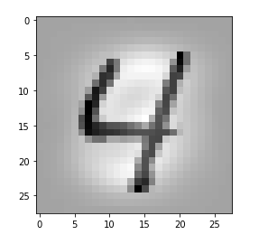
It may be necessary later on to depict a chosen input image for our analysis – e.g. a MNIST image of the test data set. How can we do this? We just fill a new Jupyter cell with the following code:
ay_img = test_imgs[7:8]
plt.imshow(ay_img[0,:,:,0], cmap=plt.cm.binary)
This code lines would plot the eighths sample image of the already shuffled test data set.
Using layer names and saving as well as restoring a model
We first must extend our previously defined functions to be able to deal with layer names. We change the code in our Jupyter Cell 8 (see the last article) in the following way:
Jupyter Cell 8: Setting up a training run
# Perform a training run
# ********************

# Prepare the plotting
# The really important command for interactive (=interediate) plot updating
%matplotlib notebook
plt.ion()

#sizing
fig_size = plt.rcParams["figure.figsize"]
fig_size[0] = 8
fig_size[1] = 3

# One figure
# -----------
fig1 = plt.figure(1)
#fig2 = plt.figure(2)

# first figure with two plot-areas with axes
# --------------------------------------------
ax1_1 = fig1.add_subplot(121)
ax1_2 = fig1.add_subplot(122)
fig1.canvas.draw()

# second figure with just one plot area with axes
# -------------------------------------------------
#ax2 = fig2.add_subplot(121)
#ax2_1 = fig2.add_subplot(121)
#ax2_2 = fig2.add_subplot(122)
#fig2.canvas.draw()

# ~~~~~~~~~~~~~~~~~~~~~~~~~~~~~~~~~~~~~~~~~~~~~
# Parameterization of the training run

#build = False
build = True
if cnn == None:
    build = True
    x_optimizer = None
batch_size=64
epochs=80
reset = False
#reset = True # we want training to start again with the initial weights

nmy_loss    ='categorical_crossentropy'
my_metrics =['accuracy']

my_regularizer = None
my_regularizer = 'l2'
my_reg_param_l2 = 0.001
#my_reg_param_l2 = 0.01
my_reg_param_l1 = 0.01


my_optimizer      = 'rmsprop'       # Present alternatives:  rmsprop, nadam, adamax
my_momentum       = 0.5           # momentum value
my_lr_sched       = 'powerSched'    # Present alternatrives: None, powerSched, exponential
#my_lr_sched       = None           # Present alternatrives: None, powerSched, exponential
my_lr_init        = 0.001           # initial leaning rate
my_lr_decay_steps = 1               # decay steps = 1
my_lr_decay_rate  = 0.001           # decay rate


li_conv_1    = [32, (3,3), 0]
li_conv_2    = [64, (3,3), 0]
li_conv_3    = [128, (3,3), 0]
li_Conv      = [li_conv_1, li_conv_2, li_conv_3]
li_Conv_Name = ["Conv2D_1", "Conv2D_2", "Conv2D_3"]
li_pool_1    = [(2,2)]
li_pool_2    = [(2,2)]
li_Pool      = [li_pool_1, li_pool_2]
li_Pool_Name = ["Max_Pool_1", "Max_Pool_2", "Max_Pool_3"]
li_dense_1   = [100, 0]
#li_dense_2  = [30, 0]
li_dense_3   = [10, 0]
li_MLP       = [li_dense_1, li_dense_2, li_dense_3]
li_MLP       = [li_dense_1, li_dense_3]
input_shape  = (28,28,1)

try:
    if gpu:
        with tf.device("/GPU:0"):
            cnn, fit_time, history, x_optimizer  = train( cnn, build, train_imgs, train_labels,
                                            li_Conv, li_Conv_Name, li_Pool, li_Pool_Name, li_MLP, input_shape,
                                            reset, epochs, batch_size,
                                            my_loss=my_loss, my_metrics=my_metrics,
                                            my_regularizer=my_regularizer,
                                            my_reg_param_l2=my_reg_param_l2, my_reg_param_l1=my_reg_param_l1,
                                            my_optimizer=my_optimizer, my_momentum = 0.8,
                                            my_lr_sched=my_lr_sched,
                                            my_lr_init=my_lr_init, my_lr_decay_steps=my_lr_decay_steps,
                                            my_lr_decay_rate=my_lr_decay_rate,
                                            fig1=fig1, ax1_1=ax1_1, ax1_2=ax1_2
                                            )
        print('Time_GPU: ', fit_time)
    else:
        with tf.device("/CPU:0"):
            cnn, fit_time, history = train( cnn, build, train_imgs, train_labels,
                                            li_Conv, li_Conv_Name, li_Pool, li_Pool_Name, li_MLP, input_shape,
                                            reset, epochs, batch_size,
                                            my_loss=my_loss, my_metrics=my_metrics,
                                            my_regularizer=my_regularizer,
                                            my_reg_param_l2=my_reg_param_l2, my_reg_param_l1=my_reg_param_l1,
                                            my_optimizer=my_optimizer, my_momentum = 0.8,
                                            my_lr_sched=my_lr_sched,
                                            my_lr_init=my_lr_init, my_lr_decay_steps=my_lr_decay_steps,
                                            my_lr_decay_rate=my_lr_decay_rate,
                                            fig1=fig1, ax1_1=ax1_1, ax1_2=ax1_2
                                            )
        print('Time_CPU: ', fit_time)
except SystemExit:
    print("stopped due to exception")
You see that I added a list
li_Conv_Name = [“Conv2D_1”, “Conv2D_2”, “Conv2D_3”]
…
li_Pool_Name = [“Max_Pool_1”, “Max_Pool_2”, “Max_Pool_3”]
which provides names of the (presently three) defined convolutional and (presently two) pooling layers. The interface to the training function has, of course, to be extended to accept these arrays. The function “train()” in Jupyter cell 7 (see the last article) is modified accordingly:
Jupyter cell 7: Trigger (re-) building and training of the CNN
# Training 2 - with test data integrated
# *****************************************
def train( cnn, build, train_imgs, train_labels,
           li_Conv, li_Conv_Name, li_Pool, li_Pool_Name, li_MLP, input_shape,
           reset=True, epochs=5, batch_size=64,
           my_loss='categorical_crossentropy', my_metrics=['accuracy'],
           my_regularizer=None,
           my_reg_param_l2=0.01, my_reg_param_l1=0.01,
           my_optimizer='rmsprop', my_momentum=0.0,
           my_lr_sched=None,
           my_lr_init=0.001, my_lr_decay_steps=1, my_lr_decay_rate=0.00001,
           fig1=None, ax1_1=None, ax1_2=None
):

    if build:
        # build cnn layers - now with regularizer - 200603 rm
        cnn = build_cnn_simple( li_Conv, li_Conv_Name, li_Pool, li_Pool_Name, li_MLP, input_shape,
                                my_regularizer = my_regularizer,
                                my_reg_param_l2 = my_reg_param_l2, my_reg_param_l1 = my_reg_param_l1)

        # compile - now with lr_scheduler - 200603
        cnn = my_compile(cnn=cnn,
                         my_loss=my_loss, my_metrics=my_metrics,
                         my_optimizer=my_optimizer, my_momentum=my_momentum,
                         my_lr_sched=my_lr_sched,
                         my_lr_init=my_lr_init, my_lr_decay_steps=my_lr_decay_steps,
                         my_lr_decay_rate=my_lr_decay_rate)

        # save the inital (!) weights to be able to restore them
        cnn.save_weights('cnn_weights.h5') # save the initial weights


    # reset weights(standard)
    if reset:
        cnn.load_weights('cnn_weights.h5')

    # Callback list
    # ~~~~~~~~~~~~~
    use_scheduler = True
    if my_lr_sched == None:
        use_scheduler = False
    lr_history = LrHistory(use_scheduler)
    callbacks_list = [lr_history]
    if fig1 != None:
        epoch_plot = EpochPlot(epochs, fig1, ax1_1, ax1_2)
        callbacks_list.append(epoch_plot)

    start_t = time.perf_counter()
    if reset:
        history = cnn.fit(train_imgs, train_labels, initial_epoch=0, epochs=epochs, batch_size=batch_size, verbose=1, shuffle=True,
                  validation_data=(test_imgs, test_labels), callbacks=callbacks_list)
    else:
        history = cnn.fit(train_imgs, train_labels, epochs=epochs, batch_size=batch_size, verbose=1, shuffle=True,
                validation_data=(test_imgs, test_labels), callbacks=callbacks_list )
    end_t = time.perf_counter()
    fit_t = end_t - start_t

    # save the model
    cnn.save('cnn.h5')

    return cnn, fit_t, history, x_optimizer  # we return cnn to be able to use it by other Jupyter functions
We transfer the name-lists further on to the function “build_cnn_simple()“:
Jupyter Cell 4: Build a simple CNN
# Sequential layer model of our CNN
# ***********************************

# important !!
# ~~~~~~~~~~~
cnn = None
x_optimizers = None

# function to build the CNN
# ~~~~~~~~~~~~~~~~~~~~~~~~~~~~
def build_cnn_simple(li_Conv, li_Conv_Name, li_Pool, li_Pool_Name, li_MLP, input_shape,
                     my_regularizer=None,
                     my_reg_param_l2=0.01, my_reg_param_l1=0.01 ):

    use_regularizer = True
    if my_regularizer == None:
        use_regularizer =
False

    # activation functions to be used in Conv-layers
    li_conv_act_funcs = ['relu', 'sigmoid', 'elu', 'tanh']
    # activation functions to be used in MLP hidden layers
    li_mlp_h_act_funcs = ['relu', 'sigmoid', 'tanh']
    # activation functions to be used in MLP output layers
    li_mlp_o_act_funcs = ['softmax', 'sigmoid']

    # dictionary for regularizer functions
    d_reg = {
        'l2': regularizers.l2,
        'l1': regularizers.l1
    }
    if use_regularizer:
        if my_regularizer not in d_reg:
            print("regularizer " + my_regularizer + " not known!")
            sys.exit()
        else:
            regul = d_reg[my_regularizer]
        if my_regularizer == 'l2':
            reg_param = my_reg_param_l2
        elif my_regularizer == 'l1':
            reg_param = my_reg_param_l1


    # Build the Conv part of the CNN
    # ~~~~~~~~~~~~~~~~~~~~~~~~~~~~~~~
    num_conv_layers = len(li_Conv)
    num_pool_layers = len(li_Pool)
    if num_pool_layers != num_conv_layers - 1:
        print("\nNumber of pool layers does not fit to number of Conv-layers")
        sys.exit()
    rg_il = range(num_conv_layers)

    # Define a sequential CNN model
    # ~~~~~~~~~~~~~~~~~~~~~~~~~-----
    cnn = models.Sequential()

    # in our simple model each con2D layer is followed by a Pooling layer (with the exeception of the last one)
    for il in rg_il:
        # add the convolutional layer
        num_filters  = li_Conv[il][0]
        t_fkern_size = li_Conv[il][1]
        cact         = li_conv_act_funcs[li_Conv[il][2]]
        cname        = li_Conv_Name[il]
        if il==0:
            cnn.add(layers.Conv2D(num_filters, t_fkern_size, activation=cact, name=cname,
                                  input_shape=input_shape))
        else:
            cnn.add(layers.Conv2D(num_filters, t_fkern_size, activation=cact, name=cname))

        # add the pooling layer
        if il < num_pool_layers:
            t_pkern_size = li_Pool[il][0]
            pname        = li_Pool_Name[il]
            cnn.add(layers.MaxPooling2D(t_pkern_size, name=pname))


    # Build the MLP part of the CNN
    # ~~~~~~~~~~~~~~~~~~~~~~~~~~~~~~~
    num_mlp_layers = len(li_MLP)
    rg_im = range(num_mlp_layers)

    cnn.add(layers.Flatten())

    for im in rg_im:
        # add the dense layer
        n_nodes = li_MLP[im][0]
        if im < num_mlp_layers - 1:
            m_act   =  li_mlp_h_act_funcs[li_MLP[im][1]]
            if use_regularizer:
                cnn.add(layers.Dense(n_nodes, activation=m_act, kernel_regularizer=regul(reg_param)))
            else:
                cnn.add(layers.Dense(n_nodes, activation=m_act))
        else:
            m_act   =  li_mlp_o_act_funcs[li_MLP[im][1]]
            if use_regularizer:
                cnn.add(layers.Dense(n_nodes, activation=m_act, kernel_regularizer=regul(reg_param)))
            else:
                cnn.add(layers.Dense(n_nodes, activation=m_act))

    return cnn
The layer names are transferred to Keras via the parameter “name” of the Model’s method “model.add()” to add a layer, e.g.:
cnn.add(layers.Conv2D(num_filters, t_fkern_size, activation=cact, name=cname))
Note that all other Jupyter cells remain unchanged.
Saving and restoring a model
Predictions of a neural network require a forward propagation of an input and thus a precise definition of layers and weights. In the last article we have already seen how we save and reload weight data of a model. However, weights make only a part of the information defining a model in a certain state. For seeing the activation of certain maps of a trained model we would like to be able to reload the full model in its trained status. Keras offers a very simple method to save and reload the complete set of data for a given model-state:
cnn.save(filename.h5′)
cnnx = models.load_model(‘filename.h5’)
This statement creates a file with the name name “filename.h5” in the h5-format (for large hierarchically organized data) in our Jupyter environment. You would of course replace “filename” by a more appropriate name to characterize your saved model-state. In my combined Eclipse-Jupyter-environment the standard path for such files points to the directory where I keep my notebooks. We included a corresponding statement at the end of the function “train()”. The attentive reader has certainly noticed this fact already.
A function to build a model for the retrieval and display of the activations of maps
We now build a new function to do the plotting of the outputs of all maps of a layer.
Jupyter Cell 9 – filling a grid with output-images of all maps of a layer
# Function to plot the activations of a layer
# -------------------------------------------
# Adaption of a method originally designed by F.Chollet

def img_grid_of_layer_activation(d_img_sets, model_fname='cnn.h5', layer_name='', img_set="test_imgs", num_img=8,
                                 scale_img_vals=False):
    '''
    Input parameter:
    -----------------
    d_img_sets: dictionary with available img_sets, which contain img tensors (presently: train_imgs, test_imgs)
    model_fname: Name of the file containing the models data
    layer_name: name of the layer for which we plot the activation; the name must be known to the Keras model (string)
    image_set: The set of images we pick a specific image from (string)
    num_img: The sample number of the image in the chosen set (integer)
    scale_img_vals: False: Do NOT scale (standardize) and clip (!) the pixel values. True: Standardize the values. (Boolean)

    Hints:
    -----------------
    We assume quadratic images
    '''

    # Load a model
    cnnx = models.load_model(model_fname)

    # get the output of a certain named layer - this includes all maps
    # https://keras.io/getting_started/faq/#how-can-i-obtain-the-output-of-an-intermediate-layer-feature-extraction
    cnnx_layer_output = cnnx.get_layer(layer_name).output

    # build a new model for input "cnnx.input" and output "output_of_layer"
    # ~~~~~~~~~~~~~~~~~
    # Keras knows the required connections and intermediat layers from its tensorflow graphs - otherwise we get an error
    # The new model can make predictions for a suitable input in the required tensor form
    mod_lay = models.Model(inputs=cnnx.input, outputs=cnnx_layer_output)

    # Pick the input image from a set of respective tensors
    if img_set not in d_img_sets:
        print("img set " + img_set + " is not known!")
        sys.exit()
    # slicing to get te right tensor
    ay_img = d_img_sets[img_set][num_img:(num_img+1)]

    # Use the tensor data as input for a prediction of model "mod_lay"
    lay_activation = mod_lay.predict(ay_img)
    print("shape of layer " + layer_name + " : ", lay_activation.shape )

    # number of maps of the selected layer
    n_maps   = lay_activation.shape[-1]

    # size of an image - we assume quadratic images
    img_size = lay_activation.shape[1]

    # Only for testing: plot an image for a selected
    # map_nr = 1
    #plt.matshow(lay_activation[0,:,:,map_nr], cmap='viridis')

    # We work with a grid of images for all maps
    # ~~~~~~~~~~~~~~~----------------------------
    # the grid is build top-down (!)
with num_cols and num_rows
    # dimensions for the grid
    num_imgs_per_row = 8
    num_cols = num_imgs_per_row
    num_rows = n_maps // num_imgs_per_row
    #print("img_size = ", img_size, " num_cols = ", num_cols, " num_rows = ", num_rows)

    # grid
    dim_hor = num_imgs_per_row * img_size
    dim_ver = num_rows * img_size
    img_grid = np.zeros( (dim_ver, dim_hor) )   # horizontal, vertical matrix
    print(img_grid.shape)

    # double loop to fill the grid
    n = 0
    for row in range(num_rows):
        for col in range(num_cols):
            n += 1
            #print("n = ", n, "row = ", row, " col = ", col)
            present_img = lay_activation[0, :, :, row*num_imgs_per_row + col]

            # standardization and clipping of the img data
            if scale_img_vals:
                present_img -= present_img.mean()
                if present_img.std() != 0.0: # standard deviation
                    present_img /= present_img.std()
                    #present_img /= (present_img.std() +1.e-8)
                    present_img *= 64
                    present_img += 128
                present_img = np.clip(present_img, 0, 255).astype('uint8') # limit values to 255

            # place the img-data at the right space and position in the grid
            # ~~~~~~~~~~~~~~~~~~~~~~~~~~~~~~~~~~~~~~~~~~~~~~~~~~~~~~~~~~~~~~
            # the following is only used if we had reversed vertical direction by accident
            #img_grid[row*img_size:(row+1)*(img_size), col*img_size:(col+1)*(img_size)] = np.flip(present_img, 0)
            img_grid[row*img_size:(row+1)*(img_size), col*img_size:(col+1)*(img_size)] = present_img

    return img_grid, img_size, dim_hor, dim_ver
I explain the core parts of this code in the next two sections.
Explanation 1: A model for the prediction of the activation output of a (convolutional layer) layer
In a first step of the function “img_grid_of_layer_activation()” we load a CNN model saved at the end of a previous training run:
cnnx = models.load_model(model_fname)
The file-name “Model_fname” is a parameter. With the lines
cnnx_layer_output = cnnx.get_layer(layer_name).output
mod_lay = models.Model(inputs=cnnx.input, outputs=cnnx_layer_output)
we define a new model “cnnx” comprising all layers (of the loaded model) in between cnnx.input and cnnx_layer_output. “cnnx_layer_output” serves as an output layer of this new model “cnnx”. This model – as every working CNN model – can make predictions for a given input tensor. The output of this prediction is a tensor produced by cnnx_layer_output; a typical shape of the tensor is:
shape of layer Conv2D_1 : (1, 26, 26, 32)
From this tensor we can retrieve the size of the comprised quadratic image data.
Explanation 2: A grid to collect “image data” of the activations of all maps of a (convolutional) layer
Matplotlib can plot a grid of equally sized images. We use such a grid to collect the activation data produced by all maps of a chosen layer, which was given by its name as an input parameter.
The first statements define the number of images in a row of the grid – i.e. the number of columns of the grid. With the number of layer maps this in turn defines the required number of rows in the grid. From the number of pixel data in the tensor we can now define the grid dimensions in terms of pixels. The double loop eventually fills in the image data extracted from the tensors produced by the layer maps.
If requested by a function parameter “scale_img_vals=True” we standardize the image data and limit the pixel values to a maximum of 255 (clipping). This can in some cases be useful to get a better graphical representation of the
activation data with some color maps.
Our function “mg_grid_of_layer_activation()” returns the grid and dimensional data.
Note that the grid is oriented from its top downwards and from the left to the right side.
Plotting the output of a layer
In a further Jupyter cell we prepare and perform a call of our new function. Afterwards we plot resulting information in two figures.
Jupyter Cell 10 – plotting the activations of a layer
# Plot the img grid of a layers activation
# ~~~~~~~~~~~~~~~~~~~~~~~~~~~~~~~~~~~~~~~~~

# global dict for the image sets
d_img_sets= {'train_imgs':train_imgs, 'test_imgs':test_imgs}

# layer - pick one of the names which you defined for your model
layer_name = "Conv2D_1"

# choose a image_set and an img number
img_set = "test_imgs"
num_img = 19


# Two figures
# -----------
fig1 = plt.figure(1)  # figure for th einput img
fig2 = plt.figure(2)  # figure for the activation outputs of th emaps

ay_img = test_imgs[num_img:num_img+1]
plt.imshow(ay_img[0,:,:,0], cmap=plt.cm.binary)

# getting the img grid
img_grid, img_size, dim_hor, dim_ver = img_grid_of_layer_activation(
                                        d_img_sets, model_fname='cnn.h5', layer_name=layer_name,
                                        img_set=img_set, num_img=num_img,
                                        scale_img_vals=False)
# Define reasonable figure dimensions by scaling the grid-size
scale = 1.6 / (img_size)
fig2 = plt.figure( figsize=(scale * dim_hor, scale * dim_ver) )
#axes
ax = fig2.gca()
ax.set_xlim(-0,dim_hor-1.0)
ax.set_ylim(dim_ver-1.0, 0)  # the grid is oriented top-down
#ax.set_ylim(-0,dim_ver-1.0) # normally wrong

# setting labels - tick positions and grid lines
ax.set_xticks(np.arange(img_size-0.5, dim_hor, img_size))
ax.set_yticks(np.arange(img_size-0.5, dim_ver, img_size))
ax.set_xticklabels([]) # no labels should be printed
ax.set_yticklabels([])

# preparing the grid
plt.grid(b=True, linestyle='-', linewidth='.5', color='#ddd', alpha=0.7)

# color-map
#cmap = 'viridis'
#cmap = 'inferno'
#cmap = 'jet'
cmap = 'magma'

plt.imshow(img_grid, aspect='auto', cmap=cmap)
The first figure contains the original MNIST image. The second figure will contain the grid with its images of the maps’ output. The code is straightforward; the corrections of the dimensions have to do with the display of intermittent lines to separate the different images. Statements like “ax.set_xticklabels([])” set the tick-mark-texts to empty strings. At the end of the code we choose a color map.
Note that I avoided to standardize the image data. Clipping suppresses extreme values; however, the map-related filters react to these values. So, let us keep the full value spectrum for a while …
Training run to get a reference model
I performed a training run with the following setting and saved the last model:
build = True
if cnn == None:
    build = True
    x_optimizer = None
batch_size=64
epochs=80
reset = False # we want training to start again with the initial weights
#reset = True # we want training to start again with the initial weights

my_loss    ='categorical_crossentropy'
my_metrics =['accuracy']

my_regularizer = None
my_regularizer = 'l2'
my_reg_param_l2 = 0.001
#my_reg_param_l2 = 0.01
my_reg_param_l1 = 0.01


my_optimizer      = 'rmsprop'       # Present alternatives:  rmsprop, nadam, adamax
my_momentum       = 0.5           # momentum value
my_lr_sched       = 'powerSched'    # Present alternatrives:
None, powerSched, exponential
#my_lr_sched       = None           # Present alternatrives: None, powerSched, exponential
my_lr_init        = 0.001           # initial leaning rate
my_lr_decay_steps = 1               # decay steps = 1
my_lr_decay_rate  = 0.001           # decay rate


li_conv_1    = [32, (3,3), 0]
li_conv_2    = [64, (3,3), 0]
li_conv_3    = [128, (3,3), 0]
li_Conv      = [li_conv_1, li_conv_2, li_conv_3]
li_Conv_Name = ["Conv2D_1", "Conv2D_2", "Conv2D_3"]
li_pool_1    = [(2,2)]
li_pool_2    = [(2,2)]
li_Pool      = [li_pool_1, li_pool_2]
li_Pool_Name = ["Max_Pool_1", "Max_Pool_2", "Max_Pool_3"]
li_dense_1   = [100, 0]
#li_dense_2  = [30, 0]
li_dense_3   = [10, 0]
li_MLP       = [li_dense_1, li_dense_2, li_dense_3]
li_MLP       = [li_dense_1, li_dense_3]
input_shape  = (28,28,1)
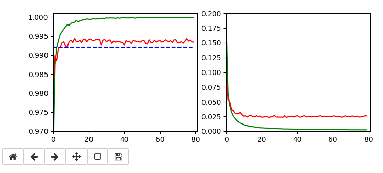
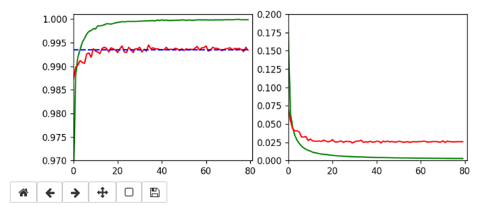
This run gives us the following results:
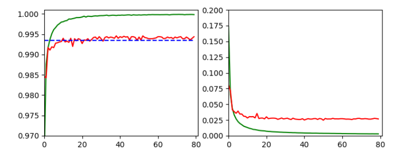
and
Epoch 80/80
933/938 [============================>.] - ETA: 0s - loss: 0.0030 - accuracy: 0.9998
present lr:  1.31509732e-05
present iteration: 75040
938/938 [==============================] - 4s 5ms/step - loss: 0.0030 - accuracy: 0.9998 - val_loss: 0.0267 - val_accuracy: 0.9944
Tests and first impressions of the convolutional layer output
Ok, let us test the code to plot the maps’ output. For the input data
# layer - pick one of the names which you defined for your model
layer_name = "Conv2D_1"

# choose a image_set and an img number
img_set = "test_imgs"
num_img = 19
we get the following results:
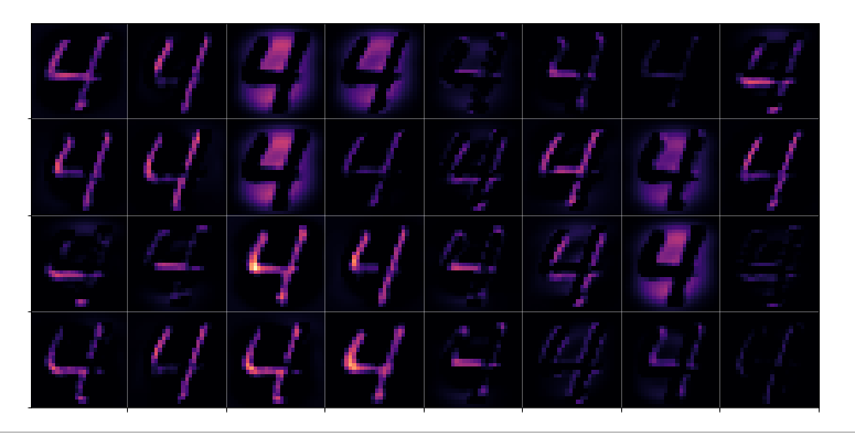
Layer “Conv2D_1”
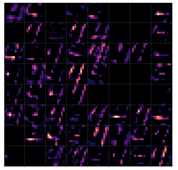
Layer “Conv2D_2”
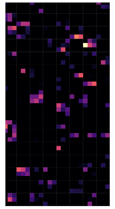
Layer “Conv2D_3”
Conclusion
Keras’ flexibility regarding model definitions allows for the definition of new models based on parts of the original CNN. The output layer of these new models can be set to any of the convolutional or pooling layers. With predictions for an input image we can extract the activation results of all maps of a layer. These data can be visualized in form of a grid that shows the reaction of a layer to the input image. A first test shows that the representations of the input get more and more abstract with higher convolutional layers.
In the next article
A simple CNN for the MNIST dataset – V – about the difference of activation patterns and features
we shall have a closer look of what these abstractions may mean for the classification of certain digit images.