Deep Dreams of a CNN trained on MNIST data – III – catching dream patterns at smaller length scales

In the first two articles of this series on Convolutional Neural Networks [CNNs] and “Deep Dream” pictures

Deep Dreams of a CNN trained on MNIST data – II – some code for pattern carving
Deep Dreams of a CNN trained on MNIST data – I – a first approach based on one selected map of a convolutional layer

I introduced the concept of CNN-based “pattern carving” and a related algorithm; it consists of a small number of iterations over of a sequence of image manipulation steps (downscaling to a resolution the CNN can handle, detection and amplification of a map triggering pattern by a CNN, upscaling to the original size and normalization). The included pattern detection and amplification algorithm is nothing else than the OIP-algorithm, which I discussed in another article series on CNNs in this blog. The OIP-algorithm is able to create a pattern, which triggers a chosen CNN map optimally, out of a chaotic fluctuation background. The difference is that we apply such an OIP-algorithms now to a structured input image – the basis for a “dream”. The “carving algorithm” is just a simplifying variation of more advanced Deep Dream algorithms; it can be combined with simple CNNs trained on gray and low-resolution images.

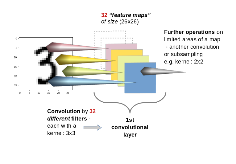
In the last article I provided some code which creates dream like pictures with the help of carving by a CNN trained on MNIST data. Nice, but … In the original theory of “Deep Dreaming” people from Google and others applied their algorithms to a cascade of so called “octaves“: Octaves represent the structures within an image at different levels of resolution. Unfortunately, at first sight, such an approach seems to be beyond the capabilities of our MNIST CNN, because the latter works on a fixed and very coarse resolution scale of 28×28 pixels, only.

As we cannot work on different scales of resolution directly: Can we handle pattern detection and amplification on different length scales in a different way? Can we somehow extend the carving process to smaller length scales and a possible detection of smaller map-triggering patterns within the input image?
The answer in short is: Yes, we can.
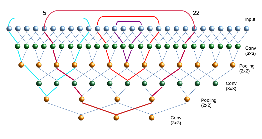
We “just” have to replace working with “octaves” by looking at sub-segments of the images – and apply our “carving” algorithm with up and down-scaling to these sub-segments as well as to the full image during an iteration process. We shall test the effects of such an approach in this article for a single selected sub-area of the input image, before we apply it more thoroughly to different input images in further articles.

A first step towards Deep Dreams “dreaming” detail structures of a chosen image …

We again use the image of a bunch of roses, which we worked with in the last articles, as a starting point for the creation of a Deep Dream picture. The easiest way to define sub-areas of our (quadratic) input image is to divide it into 4 (quadratic) adjacent sub-segments or sub-images, each with half of the side length of the original image. We thus get two rows, each with two neighboring sub-areas of the size 280×280 px. Then we could apply the carving algorithm to one selected or to all of the sub-segments. But how do we combine such an approach with an overall treatment of the full image? The answer is that we have to work in parallel on both length-scales involved. We can do this within each cycle of down- and up-scaling according to the following scheme:

  • Step 1: Pick the input image IMG at the full working size (here 560 x 560 px) – and reshape it into a tensor suitable for
    Tensorflow 2 [TF2] functions.
  • Step 2: Down- and upscale the input image “IMG” (560×560 => 28×28 => 560×560) – with information loss
  • Step 3: Calculate the difference between the re-up-scaled image to the original image as a tensor for later detail corrections.
  • Step 4: Subdivide IMG into 4 quadrants (each with a size of of 280×280 px). Save the quadrants as sub-images S_IMG_1, …. S_IMG_4 – and create respective tensors.
  • Step 5: For all sub-images: Down- and up-scale the sub-images S_IMG_m (280×280 => 28×28 => 280×280) – with information loss.
  • Step 6: For all sub-images: Determine the differences between the re-upscaled sub-images and the original sub-images as tensors for later detail corrections.
  • Step 7: Loop A [around 4 to 6 iterations]
    • Step LA-1: Pick the down-scaled image IMG_d (of size 28×28 px) as the present input image for the CNN and the OIP-analysis
    • Step LA-2: Apply the OIP-algorithm for N epochs (20 < N < 40) to the downscaled image IMG_d (28x28)
    • Step LA-3: Upscale the resulting changed version of image IMG_d to the original IMG- size by bicubic interpolation => IMG_u
    • Step LA-4: Add the (constant) correction tensor for details to IMG_u.
    • (Step LA-5: Loop B over Sub-Images)
      • Step LB-1: Cut out the area corresponding to sub-image S_IMG_m from the changed full image IMG_u. Use it as Sub_IMG_m during the following steps.
      • Step LB-2: Downscale the present sub-image Sub_IMG_m to the size suitable for the CNN (here: 28×28) by bicubic interpolation => Sub_IMG_M_d.
      • Step LB-3: Apply the OIP-algorithm for N epochs (20 < N < 40) to the downscaled sub-image (28x28) Sub_IMG_m_d
      • Step LB-4: Upscale the changed Sub_IMG_m_d to the original size of Sub_Img_m by bicubic interpolation => Sub_IMG_m_u
      • Step LB-5: Add the (constant) correction tensor to the tensor for the upscaled sub-image Sub_IMG_m_u
      • Step LB-6: Replace the sub-image region of the upscaled full image IMG_u with the (corrected) sub-image Sub_IMG_m_u
      • Step LB-7: Downscale the new full image IMG_u again (to 28×28 => IMG_d) and use the resulting IMG_d for the next iteration of Loop A

The Loop B has been placed in brackets because we are going to apply the suggested technique only to a single one of the 4 sub-image quadrants in this article.

Code fragments for the sub-image preparation

The following code for a Jupyter cell prepares the quadrants of the original image IMG – here of a bunch of roses. The code is straight forward and easy to understand.

# ****************************
# Work with sub-Images  
# ************************

%matplotlib inline

import PIL
from PIL import Image, ImageOps

fig_size = plt.rcParams["figure.figsize"]
fig_size[0] = 16
fig_size[1] = 20
fig_3 = plt.figure(
3)
ax3_1_1 = fig_3.add_subplot(541)
ax3_1_2 = fig_3.add_subplot(542)
ax3_1_3 = fig_3.add_subplot(543)
ax3_1_4 = fig_3.add_subplot(544)
ax3_2_1 = fig_3.add_subplot(545)
ax3_2_2 = fig_3.add_subplot(546)
ax3_2_3 = fig_3.add_subplot(547)
ax3_2_4 = fig_3.add_subplot(548)
ax3_3_1 = fig_3.add_subplot(5,4,9)
ax3_3_2 = fig_3.add_subplot(5,4,10)
ax3_3_3 = fig_3.add_subplot(5,4,11)
ax3_3_4 = fig_3.add_subplot(5,4,12)
ax3_4_1 = fig_3.add_subplot(5,4,13)
ax3_4_2 = fig_3.add_subplot(5,4,14)
ax3_4_3 = fig_3.add_subplot(5,4,15)
ax3_4_4 = fig_3.add_subplot(5,4,16)
ax3_5_1 = fig_3.add_subplot(5,4,17)
ax3_5_2 = fig_3.add_subplot(5,4,18)
ax3_5_3 = fig_3.add_subplot(5,4,19)
ax3_5_4 = fig_3.add_subplot(5,4,20)

# size to work with 
# ******************
img_wk_size = 560 

# bring the orig img down to (560, 560) 
# ***************************************
imgvc = Image.open("rosen_orig_farbe.jpg")
imgvc_wk_size = imgvc.resize((img_wk_size,img_wk_size), resample=PIL.Image.BICUBIC)
# Change to np arrays 
ay_picc = np.array(imgvc_wk_size)
print("ay_picc.shape = ", ay_picc.shape)
print("r = ", ay_picc[0,0,0],    " g = ", ay_picc[0,0,1],    " b = " , ay_picc[0,0,2] )
print("r = ", ay_picc[200,0,0],  " g = ", ay_picc[200,0,1],  " b = " , ay_picc[200,0,2] )

# Turn color to gray 
#Red * 0.3 + Green * 0.59 + Blue * 0.11
#Red * 0.2126 + Green * 0.7152 + Blue * 0.0722
#Red * 0.299 + Green * 0.587 + Blue * 0.114

ay_picc_g = ( 0.299  * ay_picc[:,:,0] + 0.587  * ay_picc[:,:,1] + 0.114  * ay_picc[:,:,2] )  
ay_picc_g = ay_picc_g.astype('float32') 
t_picc_g  = ay_picc_g.reshape((1, img_wk_size, img_wk_size, 1))
t_picc_g  = tf.image.per_image_standardization(t_picc_g)

# downsize to (28,28)  
t_picc_g_28 = tf.image.resize(t_picc_g, [28,28], method="bicubic", antialias=True)
t_picc_g_28 = tf.image.per_image_standardization(t_picc_g_28)

# get the correction for the full image 
t_picc_g_wk_size = tf.image.resize(t_picc_g_28, [img_wk_size,img_wk_size], method="bicubic", antialias=True)
t_picc_g_wk_size = tf.image.per_image_standardization(t_picc_g_wk_size)

t_picc_g_wk_size_corr = t_picc_g - t_picc_g_wk_size
t_picc_g_wk_size_re   = t_picc_g_wk_size + t_picc_g_wk_size_corr


# Display wk_size orig images  
ax3_1_1.imshow(imgvc_wk_size)
ax3_1_2.imshow(t_picc_g[0,:,:,0], cmap=plt.cm.gray)
ax3_1_3.imshow(t_picc_g_28[0,:,:,0], cmap=plt.cm.gray)
ax3_1_4.imshow(t_picc_g_wk_size_re[0,:,:,0], cmap=plt.cm.gray)


# Split in 4 sub-images 
# ***********************

half_wk_size  = int(img_wk_size / 2)  

t_picc_g_1  = t_picc_g[:, 0:half_wk_size, 0:half_wk_size, :]
t_picc_g_2  = t_picc_g[:, 0:half_wk_size, half_wk_size:img_wk_size, :]
t_picc_g_3  = t_picc_g[:, half_wk_size:img_wk_size, 0:half_wk_size, :]
t_picc_g_4  = t_picc_g[:, half_wk_size:img_wk_size, half_wk_size:img_wk_size, :]

# Display wk_size orig images  
ax3_2_1.imshow(t_picc_g_1[0,:,:,0], cmap=plt.cm.gray)
ax3_2_2.imshow(t_picc_g_2[0,:,:,0], cmap=plt.cm.gray)
ax3_2_3.imshow(t_picc_g_3[0,:,:,0], cmap=plt.cm.gray)
ax3_2_4.imshow(t_picc_g_4[0,:,:,0], cmap=plt.cm.gray)


# Downscale sub-images 
t_picc_g_1_28 = tf.image.resize(t_picc_g_1, [28,28], method="bicubic", antialias=True)
t_picc_g_2_28 = tf.image.resize(t_picc_g_2, [28,28], method="bicubic", antialias=True)
t_picc_g_3_28 = tf.image.resize(t_picc_g_3, [28,28], method="bicubic", antialias=True)
t_picc_g_4_28 = tf.image.resize(t_picc_g_4, [28,28], method="bicubic", antialias=True)


# Display downscales sub-images  
ax3_3_1.imshow(t_picc_g_1_28[0,:,:,0], cmap=plt.cm.gray)
ax3_3_2.imshow(t_picc_g_2_28[0,:,:,0], cmap=plt.cm.gray)
ax3_3_3.imshow(t_picc_g_3_28[0,:,:,0], cmap=plt.cm.gray)
ax3_3_4.imshow(t_picc_g_4_28[0,:,:,0], cmap=plt.cm.gray)


# get correction values for upsizing 
t_picc_g_1_wk_half = tf.image.resize(t_picc_g_1_28, [half_wk_size,
half_wk_size], method="bicubic", antialias=True)
t_picc_g_1_wk_half = tf.image.per_image_standardization(t_picc_g_1_wk_half)
t_picc_g_2_wk_half = tf.image.resize(t_picc_g_2_28, [half_wk_size,half_wk_size], method="bicubic", antialias=True)
t_picc_g_2_wk_half = tf.image.per_image_standardization(t_picc_g_2_wk_half)
t_picc_g_3_wk_half = tf.image.resize(t_picc_g_3_28, [half_wk_size,half_wk_size], method="bicubic", antialias=True)
t_picc_g_3_wk_half = tf.image.per_image_standardization(t_picc_g_3_wk_half)
t_picc_g_4_wk_half = tf.image.resize(t_picc_g_4_28, [half_wk_size,half_wk_size], method="bicubic", antialias=True)
t_picc_g_4_wk_half = tf.image.per_image_standardization(t_picc_g_4_wk_half)
 
    
t_picc_g_1_corr =  t_picc_g_1 - t_picc_g_1_wk_half   
t_picc_g_2_corr =  t_picc_g_2 - t_picc_g_2_wk_half   
t_picc_g_3_corr =  t_picc_g_3 - t_picc_g_3_wk_half   
t_picc_g_4_corr =  t_picc_g_4 - t_picc_g_4_wk_half   

t_picc_g_1_re   = t_picc_g_1_wk_half + t_picc_g_1_corr 
t_picc_g_2_re   = t_picc_g_2_wk_half + t_picc_g_2_corr 
t_picc_g_3_re   = t_picc_g_3_wk_half + t_picc_g_3_corr 
t_picc_g_4_re   = t_picc_g_4_wk_half + t_picc_g_4_corr 

print(t_picc_g_1_re.shape)

# Display downscales sub-images  
ax3_4_1.imshow(t_picc_g_1_re[0,:,:,0], cmap=plt.cm.gray)
ax3_4_2.imshow(t_picc_g_2_re[0,:,:,0], cmap=plt.cm.gray)
ax3_4_3.imshow(t_picc_g_3_re[0,:,:,0], cmap=plt.cm.gray)
ax3_4_4.imshow(t_picc_g_4_re[0,:,:,0], cmap=plt.cm.gray)

ay_img_comp = np.zeros((img_wk_size,img_wk_size))
ay_t_comp   = ay_img_comp.reshape((1,img_wk_size, img_wk_size,1))
t_pic_comp  = ay_t_comp
t_pic_comp[0, 0:half_wk_size, 0:half_wk_size, 0]                       = t_picc_g_1_re[0, :, :, 0]
t_pic_comp[0, 0:half_wk_size, half_wk_size:img_wk_size, 0]             = t_picc_g_2_re[0, :, :, 0]
t_pic_comp[0, half_wk_size:img_wk_size, 0:half_wk_size, 0]             = t_picc_g_3_re[0, :, :, 0]
t_pic_comp[0, half_wk_size:img_wk_size, half_wk_size:img_wk_size, 0]   = t_picc_g_4_re[0, :, :, 0]

ax3_5_1.imshow(t_picc_g[0,:,:,0], cmap=plt.cm.gray)
ax3_5_2.imshow(t_pic_comp[0,:,:,0], cmap=plt.cm.gray)

 
Note the computation of the correction tensors; we prove their effectiveness below by displaying respective results for the full image, cut out and re-upscaled, corrected quadrants and replaced areas of the original image.

The results in the prepared image frames look like:
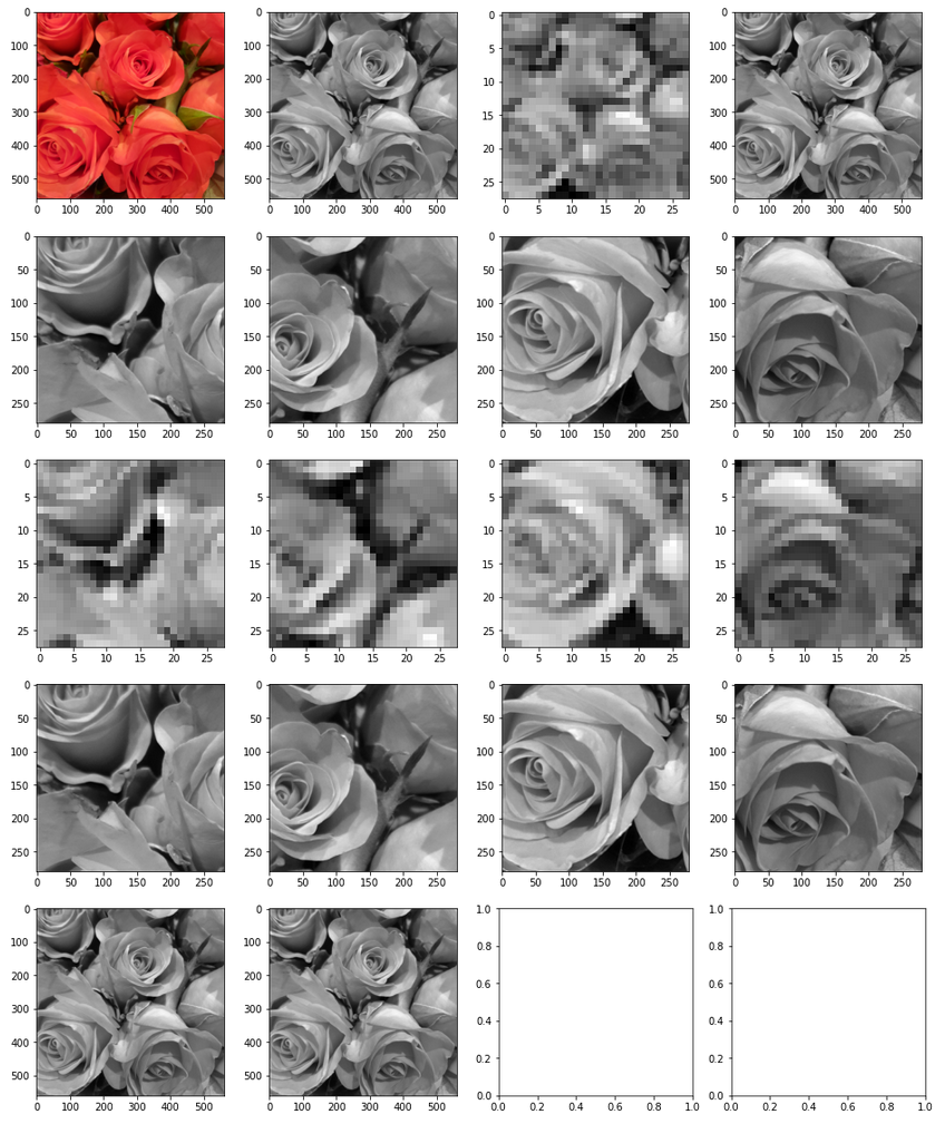
Good!

Some code for the carving algorithm – applied to the full image AND a single selected sub-image

Now, for a first test, we concentrate on the sub-image in the lower-right corner – and apply the above algorithm. A corresponding Jupyter cell code is given below:

# *************************************************************************
# OIP analysis on sub-image tiles (to be used after the previous cell)
# **************************************************************************
# Note: To be applied after previous cell !!!
# ******

#interactive plotting - will be used in a future version when we deal with "octaves" 
#%matplotlib notebook 
#plt.ion()

%matplotlib inline

# preparation of figure frames 
# ~~~~~~~~~~~~~~~~~~~~~~~~~~~~~
fig_size = plt.rcParams["figure.figsize"]
fig_size[0] = 12
fig_size[1] = 12
fig_4 = plt.figure(4)
ax4_1_1 = fig_4.add_subplot(441)
ax4_1_2 = fig_4.add_subplot(442)
ax4_1_3 = fig_4.add_subplot(443)
ax4_1_4 = fig_4.add_subplot(444)

ax4_2_1 = fig_4.add_subplot(445)
ax4_2_2 = fig_4.add_subplot(446)
ax4_2_3 = fig_4.add_subplot(447)
ax4_2_
4 = fig_4.add_subplot(448)

ax4_3_1 = fig_4.add_subplot(4,4,9)
ax4_3_2 = fig_4.add_subplot(4,4,10)
ax4_3_3 = fig_4.add_subplot(4,4,11)
ax4_3_4 = fig_4.add_subplot(4,4,12)

ax4_4_1 = fig_4.add_subplot(4,4,13)
ax4_4_2 = fig_4.add_subplot(4,4,14)
ax4_4_3 = fig_4.add_subplot(4,4,15)
ax4_4_4 = fig_4.add_subplot(4,4,16)

fig_size = plt.rcParams["figure.figsize"]
fig_size[0] = 12
fig_size[1] = 6
fig_5 = plt.figure(5)
axa5_1 = fig_5.add_subplot(241)
axa5_2 = fig_5.add_subplot(242)
axa5_3 = fig_5.add_subplot(243)
axa5_4 = fig_5.add_subplot(244)
axa5_5 = fig_5.add_subplot(245)
axa5_6 = fig_5.add_subplot(246)
axa5_7 = fig_5.add_subplot(247)
axa5_8 = fig_5.add_subplot(248)
li_axa5 = [axa5_1, axa5_2, axa5_3, axa5_4, axa5_5, axa5_6, axa5_7, axa5_8]

# Some general OIP run parameters 
# ~~~~~~~~~~~~~~~~~~~~~~~~~~~~~~~~~
n_epochs  = 30          # should be divisible by 5  
n_steps   = 6           # number of intermediate reports 
epsilon   = 0.01        # step size for gradient correction  
conv_criterion = 2.e-4  # criterion for a potential stop of optimization 

# image width parameters
# ~~~~~~~~~~~~~~~~~~~~~
img_wk_size   = 560    # must be identical to the last cell   
half_wk_size  = int(img_wk_size / 2) 

# min / max values of the input image 
#~~~~~~~~~~~~~~~~~~~~~~~~~~~~~~~~~~~~
# Note : to be used for contrast enhancement 
min1 = tf.reduce_min(t_picc_g)
max1 = tf.reduce_max(t_picc_g)
# parameters to deal with the spectral distribution of gray values
spect_dist = min(abs(min1), abs(max1))
spect_fact   = 0.85
height_fact  = 1.1

# Set the gray downscaled input image as a startng point for the iteration loop 
# ~~~~~~~~~~~~~----------~~~~--------------~~~~~~~~~~~~~~~~~~~~~~~~~~~~~~~~~~~~~~~~
MyOIP._initial_inp_img_data = t_picc_g_28

# ************
# Main Loop 
# ***********

num_main_iterate = 4
# map_index_main = -1       # take a cost function for a full layer 
map_index_main = 56         # map-index to be used for the OIP analysis of the full image  
map_index_sub  = 56         # map-index to be used for the OIP analysis of the sub-images   


for j in range(num_main_iterate):
   
    # ******************************************************
    # deal with the full (downscaled) input image 
    # ******************************************************
    
    # Apply OIP-algorithm to the whole downscaled image  
    # ~~~~~~~~~~~~~~~~~~~-----------~~~~~~~~~~~~~~~~~~~~~~~
    map_index_main_oip = map_index_main   # map-index we are interested in 

    # Perform the OIP analysis 
    MyOIP._derive_OIP(map_index = map_index_oip, 
                      n_epochs = n_epochs, n_steps = n_steps, 
                      epsilon = epsilon , conv_criterion = conv_criterion, 
                      b_stop_with_convergence=False,
                      b_print=False,
                      li_axa = li_axa5,
                      ax1_1 = ax4_1_1, ax1_2 = ax4_1_2)

    # display the modified downscaled image  (without and with contrast)
    # ~~~~~~~~~~~~~~~~~~~~~~~~~~~~~~~~~~~~~~
    t_oip_g_28  = MyOIP._inp_img_data
    ay_oip_g_28 = t_oip_g_28[0,:,:,0].numpy()
    ay_oip_g_28_cont = MyOIP._transform_tensor_to_img(T_img=t_oip_g_28[0,:,:,0], centre_move=0.33, fact=1.0)
    ax4_1_3.imshow(ay_oip_g_28_cont, cmap=plt.cm.gray)
    ax4_1_4.imshow(t_picc_g_28[0, :, :, 0], cmap=plt.cm.gray)
    
    # rescale to 560 and re-add details via the correction tensor  
    # ~~~~~~~~~~~~~~~~~~~~~~~~~~~~~~~~~~~~~~~~~~~~~~~~~~~~~~~~~~~~~
    t_oip_g_wk_size        = tf.image.resize(t_oip_g_28, [img_wk_size,img_wk_size], 
                                             method="bicubic", antialias=True)
    t_oip_g_wk_size_re     = t_oip_g_wk_size + t_picc_g_wk_size_corr 
    
    # standardize to get an intermediate image 
    # ~~~~~~~~~~~~~~~~~~~~~~~~~~~~~~~~~~~~~~~~~~~~
n    # t_oip_g_loop           = t_oip_g_wk_size_re.numpy()
    # t_oip_g_wk_size_re_std = tf.image.per_image_standardization(t_oip_g_wk_size_re)
    t_oip_g_wk_size_re_std = tf.image.per_image_standardization(t_oip_g_wk_size_re)
    t_oip_g_loop           = t_oip_g_wk_size_re_std.numpy()
    
    # contrast required as the reduction of irrelvant pixels has smoothed out the gray scale beneath 
    # ~~~~~~~~~~~~~~~~~
    # the added details at pattern areas = high level of whitened socket + relative small detail variation    
    t_oip_g_wk_size_re_std_plt = tf.clip_by_value(height_fact*t_oip_g_wk_size_re_std, -spect_dist*spect_fact, spect_dist*spect_fact)
    ax4_2_1.imshow(t_oip_g_wk_size[0,:,:,0], cmap=plt.cm.gray)
    ax4_2_2.imshow(t_oip_g_wk_size_re_std[0,:,:,0], cmap=plt.cm.gray)
    ax4_2_3.imshow(t_oip_g_wk_size_re_std_plt[0,:,:,0], cmap=plt.cm.gray)
    ax4_2_4.imshow(t_picc_g[0,:,:,0], cmap=plt.cm.gray)
   

    # *************************************************************
    # deal with a chosen sub-image - in this version: "t_oip_4_g"
    # **************************************************************
   
    # Cut out and downscale a sub-image region 
    # ~~~~~~~~~~~~~~~~~~~~~~~~~~~~~~~~~~~~~~~~~
    t_oip_4_g     = t_oip_g_loop[:, half_wk_size:img_wk_size, half_wk_size:img_wk_size, :]
    t_oip_4_g_28  = tf.image.resize(t_oip_4_g, [28,28], method="bicubic", antialias=True)
    
    # use the downscaled sub-image as an input image to the OIP-algorithm 
    # ~~~~~~~~~~~~~~~~~~~~~~~~~~~~~~~~~~~~~~~~~~~~~~~~~~~~~~~~~~~~~~~~~~~~
    MyOIP._initial_inp_img_data = t_oip_4_g_28
    
    
    # Perform the OIP analysis on the sub-image
    # ~~~~~~~~~~~~~~~~~~~~~~~~~~~~~~~~~~~~~~~~~~~
    map_index_sub_oip  = map_index_sub   # we may vary this in later versions 
    
    MyOIP._derive_OIP(map_index = map_index_sub_oip, 
                      n_epochs = n_epochs, n_steps = n_steps, 
                      epsilon = epsilon , conv_criterion = conv_criterion, 
                      b_stop_with_convergence=False,
                      b_print=False,
                      li_axa = li_axa5,
                      ax1_1 = ax4_3_1, ax1_2 = ax4_3_2)
    
    
    # display the modified sub-image without and with contrast  
    # ~~~~~~~~~~~~~~~~~~~~~~~~~~~~~~~~~~~~~~~~~~~~~~~~~~~~~~~~~
    t_oip_4_g_28  = MyOIP._inp_img_data
    ay_oip_4_g_28 = t_oip_4_g_28[0,:,:,0].numpy()
    ay_oip_4_g_28_cont = MyOIP._transform_tensor_to_img(T_img=t_oip_4_g_28[0,:,:,0], centre_move=0.33, fact=1.0)
    ax4_3_3.imshow(ay_oip_4_g_28_cont, cmap=plt.cm.gray)
    ax4_3_4.imshow(t_oip_4_g[0, :, :, 0], cmap=plt.cm.gray)
    
    # upscaling of the present sub-image 
    # ~~~~~~~~~~~~~~~~~~~~~~~~~~~~~~~~~~~
    t_pic_4_g_wk_half = tf.image.resize(t_oip_4_g_28, [half_wk_size,half_wk_size], method="bicubic", antialias=True)
    
    # add the detail correction to the manipulated upscaled sub-image
    # ~~~~~~~~~~~~~~~~~~~~~~~~~~~~~~~~~~~~~~~~~~~~~~~~~~~~~~~~~~~~~~~~
    t_pic_4_g_wk_half = t_pic_4_g_wk_half + t_picc_g_4_corr
    #t_pic_4_g_wk_half = tf.image.per_image_standardization(t_pic_4_g_wk_half)
    ax4_4_1.imshow(t_pic_4_g_wk_half[0, :, :, 0], cmap=plt.cm.gray)
    ax4_4_2.imshow(t_oip_4_g[0, :, :, 0], cmap=plt.cm.gray)
    
    # Overwrite the related region in the full image with the new sub-image  
    # ~~~~~~~~~~~~~~~~~~~~~~~~~~~~~~~~~~~~~~~~~~~~~~~~~~~~~~~~~~~~~~~~~~~~~
    t_oip_g_loop[0, half_wk_size:img_wk_size, half_wk_size:img_wk_size, 0]  = t_pic_4_g_wk_half[0, :, :, 0]
    t_oip_g_loop_std = tf.image.per_image_standardization(t_oip_g_loop)
    
    #ax4_4_3.imshow(t_oip_g_loop[0, :, :, 0], cmap=plt.cm.gray)   
    ax4_4_3.imshow(t_oip_g_loop_std[0, :, :, 0], cmap=plt.cm.gray)   
    ay_oip_g_loop_std_plt = tf.clip_by_value(height_fact*t_oip_g_loop_std, -spect_dist*spect_fact, spect_dist*spect_fact)
    ax4_4_4.
imshow(ay_oip_g_loop_std_plt[0, :, :, 0], cmap=plt.cm.gray)
    
    # Downscale the resulting new full image and feed it into into the next iteration of the main loop
    # ~~~~~~~~~~~~~~~~~~~~~~~~~~~~~~~~~~~~~~~~~~~~~~~~~~~~~~~~~~~~~~~~~~~~~~~~~~~~~~~~~~~~~~~~~~~~~~~~~
    MyOIP._initial_inp_img_data = tf.image.resize(t_oip_g_loop_std, [28,28], method="bicubic", antialias=True)


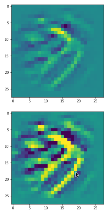
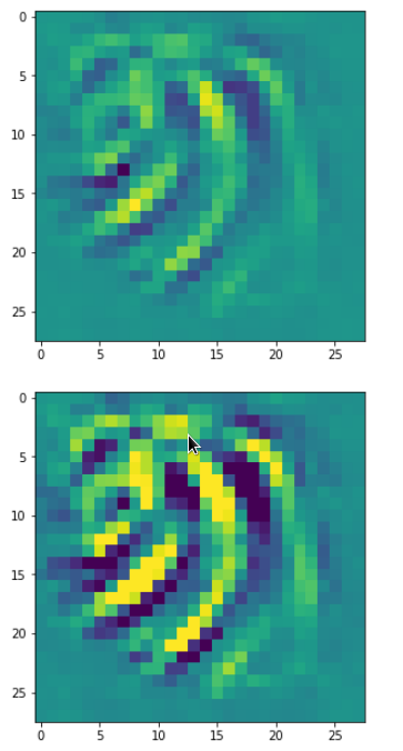
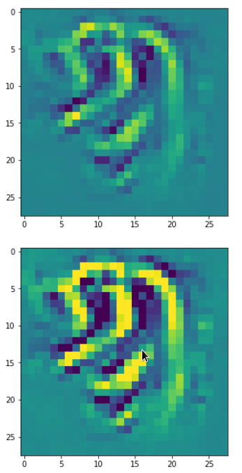
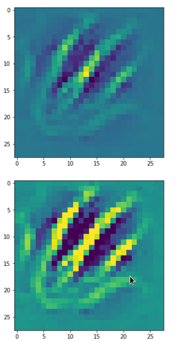
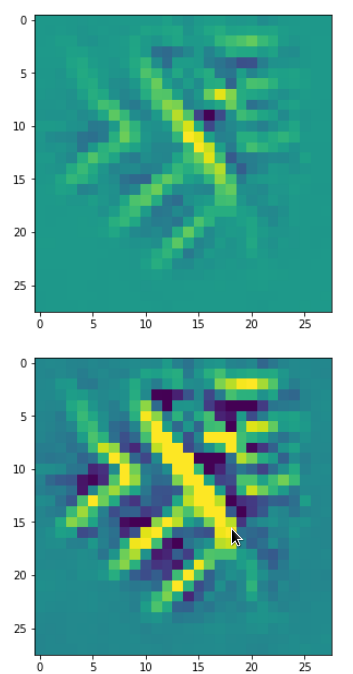
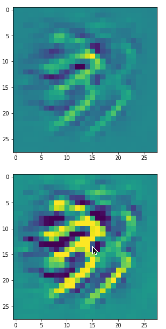
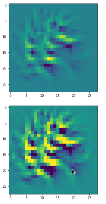
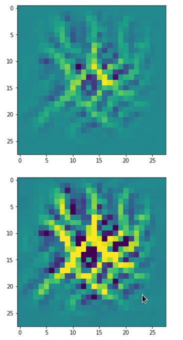
The result of these operations after 4 iterations is displayed in the following image:

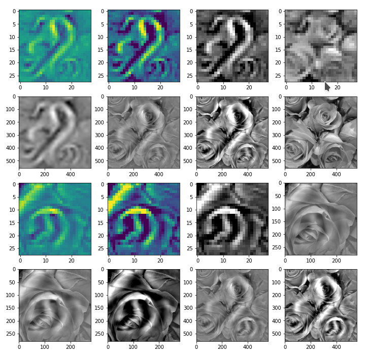
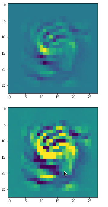
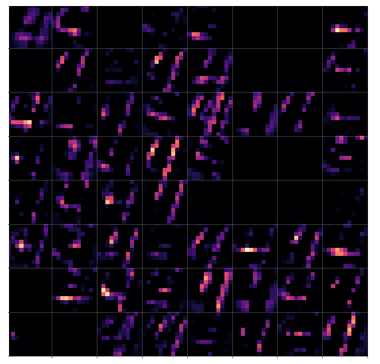
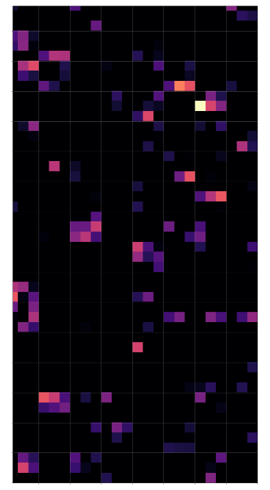
We recognize again the worm-like shape resulting for map 56, which we have seen in the last article, already. (By the way: Our CNN’s map 56 originally is strongly triggered for the shapes of handwritten 9-digits and plays a significant role in classifying respective images correctly). But there is a new feature which appeared in the lower right part of the image – a kind of wheel or two closely neighbored 9-like shapes.

The following code compares the final result with the original image:

fig_size = plt.rcParams["figure.figsize"]
fig_size[0] = 12
fig_size[1] = 12
fig_7X = plt.figure(7)
ax1_7X_1 = fig_7X.add_subplot(221)
ax1_7X_2 = fig_7X.add_subplot(222)
ax1_7X_3 = fig_7X.add_subplot(223)
ax1_7X_4 = fig_7X.add_subplot(224)

ay_pic_full_cont = MyOIP._transform_tensor_to_img(T_img=t_oip_g_loop_std[0, :, :, 0], centre_move=0.46, fact=0.8)

ax1_7X_1.imshow(imgvc_wk_size)
ax1_7X_2.imshow(t_picc_g[0,:,:,0], cmap=plt.cm.gray)
ax1_7X_3.imshow(ay_oip_g_loop_std_plt[0, :, :, 0], cmap=plt.cm.gray)
ax1_7X_4.imshow(ay_pic_full_cont, cmap=plt.cm.gray)

Giving:

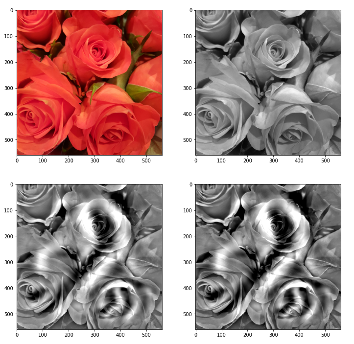
Those who do not like the relative strong contrast may do their own experiments with other parameters for contrast enhancement.

You see: Simplifying prejudices about the world, which get or got manifested in inflexible neural networks (or brains ?), may lead to strange, if not bad dreams. May also some politicians learn from this … hmmm, just joking, as this requires both an openness and capacity for learning … can’t await Jan, 21st …

Conclusion

Our “carving algorithm”, which corresponds to an amplification of traces of map-related patterns that a CNN detects in an input image, can also be used for sub-image-areas and their pixel information. We can therefore use even very limited CNNs trained on low resolution MNIST images to create a “Deep MNIST Dream” out of a chosen arbitrary input image. At least in principle.

Addendum 06.01.2021: There is, however, a pitfall – our CNN (for MNIST or other image samples) may have been trained and work on standardized image/pixel data, only. But even if the overall input image may have been standardized before operating on it in the sense of the algorithm discussed in this article, we should take into account that a sub-image area may contain pixel data which are far from a standardized distribution. So, our corrections for details may require more than just the calculation of a difference term. We may have to reverse intermediate standardization steps, too. We shall take care of this in forthcoming code changes.

In the next article we are going to extend our algorithm to multiple cascaded sub-areas of our image – and we vary the maps used for different sub-areas at the same time.


A simple CNN for the MNIST dataset – VII – outline of steps to visualize image patterns which trigger filter maps

During my present article series on a simple CNN we have seen how we set up and train such an artificial neural network with the help of Keras.

A simple CNN for the MNIST dataset – VI – classification by activation patterns and the role of the CNN’s MLP part
A simple CNN for the MNIST dataset – V – about the difference of activation patterns and features
A simple CNN for the MNIST dataset – IV – Visualizing the activation output of convolutional layers and maps
A simple CNN for the MNIST dataset – III – inclusion of a learning-rate scheduler, momentum and a L2-regularizer
A simple CNN for the MNIST datasets – II – building the CNN with Keras and a first test
A simple CNN for the MNIST datasets – I – CNN basics

Lately we managed to visualize the activations of the maps which constitute the convolutional layers of a CNN {Conv layer]. A Conv layer in a CNN basically is a collection of maps. The chain of convolutions produces characteristic patterns across the low dimensional maps of the last (i.e. the deepest) convolutional layer – in our case of the 3rd layer “Conv2D_3”. Such patterns obviously improve the classification of images with respect to their contents significantly in comparison to pure MLPs. I called a node activation pattern within or across CNN maps a FCP (see the fifth article of this series).

The map activations of the last convolutional layer are actually evaluated by a MLP, whose dense layer we embedded in our CNN. In the last article we therefore also visualized the activation values of the nodes within the first dense MLP-layer. We got some indications that map activation patterns, i.e. FCPs, for different image classes indeed create significantly different patterns within the MLP – even when the human eye does not directly see the decisive difference in the FCPs in problematic and confusing cases of input images.

In so far the effect of the transformation cascade in the convolutional parts of a CNN is somewhat comparable to the positive effect of a cluster analysis of MNIST images ahead of a MLP classification. Both approaches correspond to a projection of the input data into lower dimensional representation spaces and provide clearer classification patterns to the MLP. However, convolutions do a far better job to produce distinguished patterns for a class of images than a simple cluster analysis. The assumed reason is that chained convolutions somehow identify characteristic patterns within the input images themselves.

Is there a relation between a FCP and a a pattern in the pixel distribution of the input image?

But so far, we did not get any clear idea about the relation of FCP-patterns with pixel patterns in the original image. In other words: We have no clue about what different maps react to in terms of characteristic patterns in the input images. Actually, we do not even have a proof that a specific map – or more precisely the activation of a specific map – is triggered by some kind of distinct pattern in the value distribution for the original image pixels.

I call an original pattern to which a CNN map strongly reacts to an OIP; an OIP thus represents a certain geometrical pixel constellation in the input image which activates neurons in a specific map very strongly. Not more, not less. Note that an OIP therefore represents an idealized pixel constellation – a pattern which at best is free of any disturbances which might reduce the activation of a specific map. Can we construct an image with just the required OIP pixel constellation to trigger a map optimally? Yes, we can – at least approximately.

In the present article I shall outline the required steps which will enable us to visualize OIPs later on. In my opinion this is an important step to understand the abilities of CNNs a bit better. In particular it helps to clarify whether and in how far the term “feature detection” is appropriate. In our case we look out for primitive patterns in the multitude of MNIST images of handwritten digits. Handwritten digits are interesting objects regarding basic patterns – especially as we humans have some very clear abstract and constructive concepts in mind when we speak about basic primitive elements of digit notations – namely line and bow segments which get arranged in specific ways to denote a digit.

At the end of this article we shall have a first look at some OIP patterns which trigger a few chosen individual maps of the third convolutional layer of our CNN. In the next article I shall explain required basic code elements to create such OIP pictures. Subsequent articles will refine and extend our methods towards a more systematic analysis.

Questions and objectives

We shall try to answer a series of questions to approach the subject of OIPs and features:

  • How can Keras help us to find and visualize an OIP which provokes a maximum average reaction of a map?
  • How well is the “maximum” defined with respect to input data of our visualization method?
  • Do we recognize sub-patterns in such OIPs?
  • How do the OIPs – if there are any – reflect a translational invariance of complex, composed patterns?
  • What does a maximum activation of an individual node of a map mean in terms of an input pattern?

What do I mean by “maximum average reaction“? A specific map of a CNN corresponds to a 2-dim array of “neurons” whose activation functions produce some output. The basic idea is that we want to achieve a maximum average value of this output by systematically optimizing initially random input image data until, hopefully, a pattern emerges.

Basic strategy to visualize an OIP pattern

In a way we shall try to create order out of chaos: We want to systematically modify an initial random distribution of pixel values until we reach a maximum activation of the chosen map. We already know how to systematically approach a minimum of a function depending on a multidimensional arrangement of parameters. We apply the “gradient descent” method to a hyperplane created by a suitable loss-function. Considering the basic principles of “gradient descent” we may safely assume that a slightly modified gradient guided approach will also work for maxima. This in turn means:

We must define a map-specific “loss” function which approaches a maximum value for optimum node activation. A suitable simple function could be a sum or average increasing with the activation values of the map’s nodes. So, in contrast to classification tasks we will have to use a “gradient ascent” method- The basic idea and a respective simple technical method is e.g. described in the book of F. Chollet (Deep Learning mit Python und Keras”, 2018, mitp Verlag; I only have the German book version, but the original is easy to find).

But what is varied in such an optimization model? Certainly not the weights of the already trained CNN! The variation happens with respect to the input data – the initial pixel values of the input image are corrected by the gradient values of the loss function.

Next question: What do we choose as a starting point of the optimization process? Answer: Some kind of random distribution of pixel values. The basic hope is that a gradient ascent method searching for a maximum of a loss function would also “converge“.

Well, here began my first problem: Converge in relation to what exactly? With respect to exactly one input input image or to multiple input images with different initial statistical distributions of pixel data? With fluctuations defined on different wavelength levels? (Physicists and mathematicians automatically think of a Fourier transformation at this point 🙂 ). This corresponds to the question whether a maximum found for a certain input image really is a global maximum. Actually, we shall see that the meaning of convergence is a bit fuzzy in our present context and not as well defined as in the case of a CNN-training.

To discuss fluctuations in statistical patterns at different wavelength is not so far-fetched as it may seem: Already the basic idea that a map reacts to a structured and maybe sub-structured OIP indicates that pixel correlations or variations on different length scales might play a role in triggering a map. We shall see that some maps do not react to certain “random” patterns at all. And do not forget that pooling operations induce the analysis of long range patterns by subsequent convolutional filters. The relevant wavelength is roughly doubled by each of our pooling operations! So, filters at deep convolutional layers may exclude patterns which do not show some long range characteristics.

The simplified approach discussed by Chollet assumes statistical variations on the small length scale of neighboring pixels; he picks a random value for each and every pixel of his initial input images without any long range correlations. For many maps this approach will work reasonably well and will give us a basic idea about the average pattern or, if you absolutely want to use the expression, “feature”, which a CNN-map reacts to. But being able to vary the length scale of pixel values of input images will help us to find patterns for sensitive maps, too.

We may not be able to interpret a specific activation pattern within a map; but to see what a map on average and what a single node of a map reacts to certainly would mean some progress in understanding the relation between OIPs and FCPs.

An example

The question what an OIP is depends on the scales you look at and also where an OIP appears within a real image. To confuse you a bit: Look at he following OIP-picture which triggered a certain map strongly:

The upper image was prepared with a plain color map, the lower with some contrast enhancement. I use this two-fold representation also later for other OIP-pictures.

Actually, it is not so clear what elementary pattern our map reacts to. Two parallel line segments with a third one crossing perpendicular at the upper end of the parallel segments?

One reason for being uncertain is that some patterns on a scale of lets say a fourth of the original image may appear at different locations in original images of the same class. If a network really learned about such reappearance of patterns the result for an optimum OIP may be a superposition of multiple elementary patterns at different locations. Look at the next two OIP pictures for the very same map – these patterns emerged from a slightly different statistical variation of the input pixel values:

Now, we recognize some elementary structures much better – namely a combination of bows with slightly different curvatures and elongations. Certainly useful to detect “3” digits, but parts of “2”s, too!

A different version of another map is given here:

Due to the large scale structure over the full height of the input this map is much better suited to detect “9”s at different places.

You see that multiple filters on different spatial resolution levels have to work together in this case to reflect one bow – and the bows elongation gets longer with their position to the right. It seems that the CNN has learned that bow elements with the given orientation on the left side of original images are smaller and have a different degree of curvature than to the right of a MNIST input image. So what is the OIP or what is the “feature” here? The superposition of multiple translationally shifted and differently elongated bows? Or just one bow?

Unexpected technical hurdles

I was a bit surprised that I met some technical difficulties along my personal way to answer the questions posed above. The first point is that only a few text book authors seem to discuss the question at all; F. Chollet being the remarkable exception and most authors in the field, also of articles on the Internet, refer to his ideas and methods. I find this fact interesting as many authors of introductory books on ANNs just talk about “features” and make strong claims about what “features” are in terms of entities and their detection by CNNs – but they do not provide any code to verify the almost magic “identification” of conceptual entities as “eyes”, “feathers”, “lips”, etc..

Then there are articles of interested guys, which appear at specialized web sites, as e.g. the really read-worthy contribution of the physicist F. Graetz: https://towardsdatascience.com/how-to-visualize-convolutional-features-in-40-lines-of-code-70b7d87b0030 on “towardsdatascience.com”. His color images of “features” within CIFAR images are impressive; you really should have a look at them.

But he as other authors usually take pre-trained nets like VGG16 and special datasets as CIFAR with images of much higher resolution than MNIST images. But I wanted to apply similar methods upon my own simple CNN and MNIST data. Although an analysis of OIPs of MNIST images will certainly not produce such nice high resolution color pictures as the ones of Graetz, it might be easier to extract and understand some basic principles out of numerical experiments.

Unfortunately, I found that I could not just follow and copy code snippets of F. Chollet. Partially this had to do with necessary changes Tensorflow 2 enforced in comparison to TF1 which was used by F. Chollet. Another problem was due to standardized MNIST images my own CNN was trained on. Disregarding the point of standardization during programming prevented convergence during the identification of OIPs. Another problem occurred with short range random value variations for the input image pixels as a starting point. Choosing independent random values for individual pixels suppresses long range variations; this in turn often leads to zero gradients for averaged artificial “costs” of maps at high layer levels.

A better suitable variant of Chollet’s code with respect to TF 2 was published by a guy named Mohamed at “https://www.kaggle.com/questions-and-answers/121398“. I try to interpret his line of thinking and coding in my forthcoming articles – so all credit belongs to him and F. Chollet. Nevertheless, as said, I still had to modify their code elements to take into account special aspects of my own trained CNN.

Basic outline for later coding

We saw already in previous articles that we can build new models with Keras and TensorFlow 2 [TF2] which connect some input layer with the output of an intermediate layer of an already defined CNN- or MLP-model. TF2 analyses the respective dependencies and allows for a forward propagation of input tensors to get the activation values ( i.e. the output values of the activation function) at the intermediate layer of the original model – which now plays the role of an output layer in the new (sub-) model.

However, TF2 can do even more for us: We can define a specific cost function, which depends on the output tensor values of our derived sub-model. TF2 will also (automatically) provide gradient values for this freshly defined loss function with respect to input values which we want to vary.

The basic steps to construct images which trigger certain maps optimally is the following:

  • We construct an initial input image filled with random noise. In the case of MNIST this input image would consist of input values on a 1-dim gray scale. We standardize the input image data as our CNN has been trained for such images.
  • We build a new model based on the layer structure of our original (trained) CNN-model: The new model connects the input-image-tensor at the input layer of the CNN with the output generated of a specific feature map at some intermediate layer after the forward propagation of the input data.
  • We define a new loss function which should show a maximum value for the map output – depending of course on optimized input image data for the chosen specific map.
  • We define a suitable (stochastic) gradient ascent method to approach the aspired maximum for corrected input image data.
  • We “inform” TF2 about the gradient’s dependencies on certain varying variables to give us proper gradient values. This step is of major importance in Tensorflow environments with activated “eager execution”. (In contrast to TF1 “eager execution” is the standard setting for TF2.)
  • We scale (= normalize) the gradient values to avoid too extreme corrections of the input data.
  • We take into account a standardization of the corrected input image data. This will support the overall convergence of our approach.
  • We in addition apply some tricks to avoid a over-exaggeration of small scale components (= high frequency components in the sense of a Fourier transform) in the input image data.

Especially the last point was new to me before I read the code of Mohamed at Kaggle. E.g. F. Chollet does not discuss this point in his book. But it is a very clever thought that one should care about low and high frequency contributions in patterns which trigger maps at deep convolutional layers. Whereas Mohamed discusses the aspect that high frequency components may guide the optimization process into overall side maxima during gradient ascent, I would in addition say that not offering long range variations already in the statistical input data may lead to a total non-activation of some maps. Actually, this maybe is an underestimated crucial point in the hunt for patterns which trigger maps – especially when we deal with low resolution input images.

Eager mode requirements

Keras originally provided a function “gradients()” which worked with TF1 graphs and non-eager execution mode. However, T2 executes code in eager mode automatically and therefore we have to use special functions to control gradients and their dependencies on changing variables (see for a description of “eager execution” https://www.tensorflow.org/guide/eager?hl=en ).

Among other things: TF2 provides a special function to “watch” variables whose variations have an impact on loss functions and gradient values with respect to a defined (new) model. (An internal analysis by TF2 of the impact of such variations is of course possible because our new sub-model is based on an already given layer structures of the original CNN-model.)

Visualization of some OIP-patterns in MNIST images as appetizers

Enough for today. To raise your appetite for more I present some images of OIPs. I only show patterns triggering maps on the third Conv-layer.

There are simple patterns:

But there are also more complex ones:

A closer look shows that the complexity results from translations and rotations of elementary patterns.

Conclusion

In this article we have outlined steps to build a program which allows the search for OIPs. The reader has noticed that I try to avoid the term “features”. First images of OIPs show that such patterns may appear a bit different in different parts of original input images. The maps of a CNN seem to take care of this. This is possible, only, if and when pixel correlations are evaluated over many input images and if thereby variations on larger spatial scales are taken into account. Then we also have images which show unique patterns in specific image regions – i.e. a large scale pattern without much translational invariance.

We shall look in more detail at such points as soon as we have built suitable Python functions. See the next post

A simple CNN for the MNIST dataset – VIII – filters and features – Python code to visualize patterns which activate a map strongly


A simple CNN for the MNIST dataset – IV – Visualizing the activation output of convolutional layers and maps

In the first three articles of this series on a (very) simple CNN for the MNIST dataset

A simple CNN for the MNIST dataset – III – inclusion of a learning-rate scheduler, momentum and a L2-regularizer
A simple CNN for the MNIST datasets – II – building the CNN with Keras and a first test
A simple CNN for the MNIST datasets – I – CNN basics

we invested some work into building layers and into the parameterization of a training run. Our rewards comprised a high accuracy value of around 99.35% and watching interactive plots during training.

But a CNN offers much more information which is worth and instructive to look at. In the first article I have talked a bit about feature detection happening via the “convolution” of filters with the original image data or the data produced at feature maps of previous layers. What if we could see what different filters do to the underlying data? Can we have a look at the output selected “feature maps” produce for a specific input image?

Yes, we can. And it is intriguing! The objective of this article is to plot images of the feature map output at a chosen convolutional or pooling layer of our CNN. This is accompanied by the hope to better understand the concept of abstract features extracted from an input image.

I follow an original idea published by F. Chollet (in his book “Deep Learning mit Python und Keras”, mitp Verlag) and adapt it to the code discussed in the previous articles.

Referring to inputs and outputs of models and layers

So far we have dealt with a complete CNN with a multitude of layers that produce intermediate tensors and a “one-hot”-encoded output to indicate the prediction for a hand-written digit represented by a MNIST image. The CNN itself was handled by Keras in form of a sequential model of defined convolutional and pooling layers plus layers of a multi-layer perceptron [MLP]. By the definition of such a “model” Keras does all the work required for forward and backward propagation steps in the background. After training we can “predict” the outcome for any new digit image which we feed into the CNN: We just have to fetch the data form th eoutput layer (at the end of the MLP) after a forward propagation with the weights optimized during training.

But now, we need something else:

We need a model which gives us the output, i.e. a 2-dimensional tensor – of a specific map of an intermediate Conv-layer as a prediction for an input image!

I.e. we want the output of a sub-model of our CNN containing only a part of the layers. How can we define such an (additional) model based on the layers of our complete original CNN-model?

Well, with Keras we can build a general model based on any (partial) graph of connected layers which somebody has set up. The input of such a model must follow rules appropriate to the receiving layer and the output can be that of a defined subsequent layer or map. Setting up layers and models can on a very basic level be done with the so called “Functional API of Keras“. This API enables us to directly refer to methods of the classes “Layer”, “Model”, “Input” and “Output”.

A model – as an instance of the Model-class – can be called like a function for its input (in tensor form) and it returns its output (in tensor form). As we deal with classes you will not be surprised over the fact that we can refer to the input-layer of a general model via the model’s instance name – let us say “cnnx” – and an instance attribute. A model has a unique input layer which later is fed by tensor input data. We can refer to this input layer via the attribute “input” of the model object. So, e.g. “cnnx.input” gives us a clear unique reference to the input layer. With the attribute “output” of a model we get a reference to the output layer.

But, how can we refer to the output of a specific layer or map of a CNN-model? If you look it up in the Keras documentation you will find that we can give each layer of a model a specific “name“. And a Keras model, of course, has a method to retrieve a reference to a layer via its name:

cnnx.get_layer(layer_name) .

Each convolutional layer of our CNN is an instance of the class “Conv2D-Layer” with an attribute “output” – this comprises the multidimensional tensor delivered by the activation function of the layer’s nodes (or units in Keras slang). Such a tensor has in general 4 axes for images:

sample-number of the batch, px width, px height, filter number

The “filter number” identifies a map of the Conv2D-layer. To get the “image”-data provided of a specific map (identified by “map-number”) we have to address the array as

cnnx.get_layer(layer_name)[sample-number, :, :, map-number]

We know already that these data are values in a certain range (here above 0, due to our choice of the activation function as “relu”).

Hint regarding wording: F. Chollet calls the output of the activation functions of the nodes of a layer or map the “activation” of the layer or map, repsectively. We shall use this wording in the code we are going to build.

Displaying a specific image

It may be necessary later on to depict a chosen input image for our analysis – e.g. a MNIST image of the test data set. How can we do this? We just fill a new Jupyter cell with the following code:

ay_img = test_imgs[7:8]
plt.imshow(ay_img[0,:,:,0], cmap=plt.cm.binary)

This code lines would plot the eighths sample image of the already shuffled test data set.

Using layer names and saving as well as restoring a model

We first must extend our previously defined functions to be able to deal with layer names. We change the code in our Jupyter Cell 8 (see the last article) in the following way:

Jupyter Cell 8: Setting up a training run

  
# Perform a training run 
# ********************

# Prepare the plotting 
# The really important command for interactive (=interediate) plot updating
%matplotlib notebook
plt.ion()

#sizing
fig_size = plt.rcParams["figure.figsize"]
fig_size[0] = 8
fig_size[1] = 3

# One figure 
# -----------
fig1 = plt.figure(1)
#fig2 = plt.figure(2)

# first figure with two plot-areas with axes 
# --------------------------------------------
ax1_1 = fig1.add_subplot(121)
ax1_2 = fig1.add_subplot(122)
fig1.canvas.draw()

# second figure with just one plot area with axes
# -------------------------------------------------
#ax2 = fig2.add_subplot(121)
#ax2_1 = fig2.add_subplot(121)
#ax2_2 = fig2.add_subplot(122)
#fig2.canvas.draw()

# ~~~~~~~~~~~~~~~~~~~~~~~~~~~~~~~~~~~~~~~~~~~~~
# Parameterization of the training run 

#build = False
build = True
if cnn == None:
    build = True
    x_optimizer = None 
batch_size=64
epochs=80
reset = False 
#reset = True # we want training to start again with the initial weights

nmy_loss    ='categorical_crossentropy'
my_metrics =['accuracy']

my_regularizer = None
my_regularizer = 'l2'
my_reg_param_l2 = 0.001
#my_reg_param_l2 = 0.01
my_reg_param_l1 = 0.01


my_optimizer      = 'rmsprop'       # Present alternatives:  rmsprop, nadam, adamax 
my_momentum       = 0.5           # momentum value 
my_lr_sched       = 'powerSched'    # Present alternatrives: None, powerSched, exponential 
#my_lr_sched       = None           # Present alternatrives: None, powerSched, exponential 
my_lr_init        = 0.001           # initial leaning rate  
my_lr_decay_steps = 1               # decay steps = 1 
my_lr_decay_rate  = 0.001           # decay rate 


li_conv_1    = [32, (3,3), 0] 
li_conv_2    = [64, (3,3), 0] 
li_conv_3    = [128, (3,3), 0] 
li_Conv      = [li_conv_1, li_conv_2, li_conv_3]
li_Conv_Name = ["Conv2D_1", "Conv2D_2", "Conv2D_3"]
li_pool_1    = [(2,2)]
li_pool_2    = [(2,2)]
li_Pool      = [li_pool_1, li_pool_2]
li_Pool_Name = ["Max_Pool_1", "Max_Pool_2", "Max_Pool_3"]
li_dense_1   = [100, 0]
#li_dense_2  = [30, 0]
li_dense_3   = [10, 0]
li_MLP       = [li_dense_1, li_dense_2, li_dense_3]
li_MLP       = [li_dense_1, li_dense_3]
input_shape  = (28,28,1)

try: 
    if gpu:
        with tf.device("/GPU:0"):
            cnn, fit_time, history, x_optimizer  = train( cnn, build, train_imgs, train_labels, 
                                            li_Conv, li_Conv_Name, li_Pool, li_Pool_Name, li_MLP, input_shape, 
                                            reset, epochs, batch_size, 
                                            my_loss=my_loss, my_metrics=my_metrics, 
                                            my_regularizer=my_regularizer, 
                                            my_reg_param_l2=my_reg_param_l2, my_reg_param_l1=my_reg_param_l1,  
                                            my_optimizer=my_optimizer, my_momentum = 0.8,  
                                            my_lr_sched=my_lr_sched, 
                                            my_lr_init=my_lr_init, my_lr_decay_steps=my_lr_decay_steps, 
                                            my_lr_decay_rate=my_lr_decay_rate,  
                                            fig1=fig1, ax1_1=ax1_1, ax1_2=ax1_2
                                            )
        print('Time_GPU: ', fit_time)  
    else:
        with tf.device("/CPU:0"):
            cnn, fit_time, history = train( cnn, build, train_imgs, train_labels, 
                                            li_Conv, li_Conv_Name, li_Pool, li_Pool_Name, li_MLP, input_shape, 
                                            reset, epochs, batch_size, 
                                            my_loss=my_loss, my_metrics=my_metrics, 
                                            my_regularizer=my_regularizer, 
                                            my_reg_param_l2=my_reg_param_l2, my_reg_param_l1=my_reg_param_l1,  
                                            my_optimizer=my_optimizer, my_momentum = 0.8, 
                                            my_lr_sched=my_lr_sched, 
                                            my_lr_init=my_lr_init, my_lr_decay_steps=my_lr_decay_steps, 
                                            my_lr_decay_rate=my_lr_decay_rate,  
                                            fig1=fig1, ax1_1=ax1_1, ax1_2=ax1_2
                                            )
        print('Time_CPU: ', fit_time)  
except SystemExit:
    print("stopped due to exception")

 
You see that I added a list

li_Conv_Name = [“Conv2D_1”, “Conv2D_2”, “Conv2D_3”]

li_Pool_Name = [“Max_Pool_1”, “Max_Pool_2”, “Max_Pool_3”]

which provides names of the (presently three) defined convolutional and (presently two) pooling layers. The interface to the training function has, of course, to be extended to accept these arrays. The function “train()” in Jupyter cell 7 (see the last article) is modified accordingly:

Jupyter cell 7: Trigger (re-) building and training of the CNN

# Training 2 - with test data integrated 
# *****************************************
def train( cnn, build, train_imgs, train_labels, 
           li_Conv, li_Conv_Name, li_Pool, li_Pool_Name, li_MLP, input_shape, 
           reset=True, epochs=5, batch_size=64, 
           my_loss='categorical_crossentropy', my_metrics=['accuracy'], 
           my_regularizer=None, 
           my_reg_param_l2=0.01, my_reg_param_l1=0.01, 
           my_optimizer='rmsprop', my_momentum=0.0, 
           my_lr_sched=None, 
           my_lr_init=0.001, my_lr_decay_steps=1, my_lr_decay_rate=0.00001,
           fig1=None, ax1_1=None, ax1_2=None
):
    
    if build:
        # build cnn layers - now with regularizer - 200603 rm
        cnn = build_cnn_simple( li_Conv, li_Conv_Name, li_Pool, li_Pool_Name, li_MLP, input_shape, 
                                my_regularizer = my_regularizer, 
                                my_reg_param_l2 = my_reg_param_l2, my_reg_param_l1 = my_reg_param_l1)
        
        # compile - now with lr_scheduler - 200603
        cnn = my_compile(cnn=cnn, 
                         my_loss=my_loss, my_metrics=my_metrics, 
                         my_optimizer=my_optimizer, my_momentum=my_momentum, 
                         my_lr_sched=my_lr_sched,
                         my_lr_init=my_lr_init, my_lr_decay_steps=my_lr_decay_steps, 
                         my_lr_decay_rate=my_lr_decay_rate)        
        
        # save the inital (!) weights to be able to restore them  
        cnn.save_weights('cnn_weights.h5') # save the initial weights 
         
        
    # reset weights(standard)
    if reset:
        cnn.load_weights('cnn_weights.h5')
 
    # Callback list 
    # ~~~~~~~~~~~~~
    use_scheduler = True
    if my_lr_sched == None:
        use_scheduler = False
    lr_history = LrHistory(use_scheduler)
    callbacks_list = [lr_history]
    if fig1 != None:
        epoch_plot = EpochPlot(epochs, fig1, ax1_1, ax1_2)
        callbacks_list.append(epoch_plot)
    
    start_t = time.perf_counter()
    if reset:
        history = cnn.fit(train_imgs, train_labels, initial_epoch=0, epochs=epochs, batch_size=batch_size, verbose=1, shuffle=True, 
                  validation_data=(test_imgs, test_labels), callbacks=callbacks_list) 
    else:
        history = cnn.fit(train_imgs, train_labels, epochs=epochs, batch_size=batch_size, verbose=1, shuffle=True, 
                validation_data=(test_imgs, test_labels), callbacks=callbacks_list ) 
    end_t = time.perf_counter()
    fit_t = end_t - start_t
    
    # save the model 
    cnn.save('cnn.h5')
    
    return cnn, fit_t, history, x_optimizer  # we return cnn to be able to use it by other Jupyter functions

 
We transfer the name-lists further on to the function “build_cnn_simple()“:

Jupyter Cell 4: Build a simple CNN

# Sequential layer model of our CNN
# ***********************************

# important !!
# ~~~~~~~~~~~
cnn = None
x_optimizers = None 

# function to build the CNN 
# ~~~~~~~~~~~~~~~~~~~~~~~~~~~~
def build_cnn_simple(li_Conv, li_Conv_Name, li_Pool, li_Pool_Name, li_MLP, input_shape, 
                     my_regularizer=None, 
                     my_reg_param_l2=0.01, my_reg_param_l1=0.01 ):

    use_regularizer = True
    if my_regularizer == None:
        use_regularizer = 
False  
    
    # activation functions to be used in Conv-layers 
    li_conv_act_funcs = ['relu', 'sigmoid', 'elu', 'tanh']
    # activation functions to be used in MLP hidden layers  
    li_mlp_h_act_funcs = ['relu', 'sigmoid', 'tanh']
    # activation functions to be used in MLP output layers  
    li_mlp_o_act_funcs = ['softmax', 'sigmoid']

    # dictionary for regularizer functions
    d_reg = {
        'l2': regularizers.l2,  
        'l1': regularizers.l1
    }
    if use_regularizer: 
        if my_regularizer not in d_reg:
            print("regularizer " + my_regularizer + " not known!")
            sys.exit()
        else: 
            regul = d_reg[my_regularizer] 
        if my_regularizer == 'l2':
            reg_param = my_reg_param_l2
        elif my_regularizer == 'l1':
            reg_param = my_reg_param_l1
    
    
    # Build the Conv part of the CNN
    # ~~~~~~~~~~~~~~~~~~~~~~~~~~~~~~~
    num_conv_layers = len(li_Conv)
    num_pool_layers = len(li_Pool)
    if num_pool_layers != num_conv_layers - 1: 
        print("\nNumber of pool layers does not fit to number of Conv-layers")
        sys.exit()
    rg_il = range(num_conv_layers)

    # Define a sequential CNN model
    # ~~~~~~~~~~~~~~~~~~~~~~~~~-----
    cnn = models.Sequential()

    # in our simple model each con2D layer is followed by a Pooling layer (with the exeception of the last one) 
    for il in rg_il:
        # add the convolutional layer 
        num_filters  = li_Conv[il][0]
        t_fkern_size = li_Conv[il][1]
        cact         = li_conv_act_funcs[li_Conv[il][2]]
        cname        = li_Conv_Name[il]
        if il==0:
            cnn.add(layers.Conv2D(num_filters, t_fkern_size, activation=cact, name=cname,  
                                  input_shape=input_shape))
        else:
            cnn.add(layers.Conv2D(num_filters, t_fkern_size, activation=cact, name=cname))
        
        # add the pooling layer 
        if il < num_pool_layers:
            t_pkern_size = li_Pool[il][0]
            pname        = li_Pool_Name[il] 
            cnn.add(layers.MaxPooling2D(t_pkern_size, name=pname))
            

    # Build the MLP part of the CNN
    # ~~~~~~~~~~~~~~~~~~~~~~~~~~~~~~~
    num_mlp_layers = len(li_MLP)
    rg_im = range(num_mlp_layers)

    cnn.add(layers.Flatten())

    for im in rg_im:
        # add the dense layer 
        n_nodes = li_MLP[im][0]
        if im < num_mlp_layers - 1:  
            m_act   =  li_mlp_h_act_funcs[li_MLP[im][1]]
            if use_regularizer:
                cnn.add(layers.Dense(n_nodes, activation=m_act, kernel_regularizer=regul(reg_param)))
            else:
                cnn.add(layers.Dense(n_nodes, activation=m_act))
        else: 
            m_act   =  li_mlp_o_act_funcs[li_MLP[im][1]]
            if use_regularizer:
                cnn.add(layers.Dense(n_nodes, activation=m_act, kernel_regularizer=regul(reg_param)))
            else:
                cnn.add(layers.Dense(n_nodes, activation=m_act))
                
    return cnn 

 
The layer names are transferred to Keras via the parameter “name” of the Model’s method “model.add()” to add a layer, e.g.:

cnn.add(layers.Conv2D(num_filters, t_fkern_size, activation=cact, name=cname))

Note that all other Jupyter cells remain unchanged.

Saving and restoring a model

Predictions of a neural network require a forward propagation of an input and thus a precise definition of layers and weights. In the last article we have already seen how we save and reload weight data of a model. However, weights make only a part of the information defining a model in a certain state. For seeing the activation of certain maps of a trained model we would like to be able to reload the full model in its trained status. Keras offers a very simple method to save and reload the complete set of data for a given model-state:

cnn.save(filename.h5′)
cnnx = models.load_model(‘filename.h5’)

This statement creates a file with the name name “filename.h5” in the h5-format (for large hierarchically organized data) in our Jupyter environment. You would of course replace “filename” by a more appropriate name to characterize your saved model-state. In my combined Eclipse-Jupyter-environment the standard path for such files points to the directory where I keep my notebooks. We included a corresponding statement at the end of the function “train()”. The attentive reader has certainly noticed this fact already.

A function to build a model for the retrieval and display of the activations of maps

We now build a new function to do the plotting of the outputs of all maps of a layer.

Jupyter Cell 9 – filling a grid with output-images of all maps of a layer

# Function to plot the activations of a layer 
# -------------------------------------------
# Adaption of a method originally designed by F.Chollet 

def img_grid_of_layer_activation(d_img_sets, model_fname='cnn.h5', layer_name='', img_set="test_imgs", num_img=8, 
                                 scale_img_vals=False):
    '''
    Input parameter: 
    -----------------
    d_img_sets: dictionary with available img_sets, which contain img tensors (presently: train_imgs, test_imgs)  
    model_fname: Name of the file containing the models data 
    layer_name: name of the layer for which we plot the activation; the name must be known to the Keras model (string) 
    image_set: The set of images we pick a specific image from (string)
    num_img: The sample number of the image in the chosen set (integer) 
    scale_img_vals: False: Do NOT scale (standardize) and clip (!) the pixel values. True: Standardize the values. (Boolean)
        
    Hints: 
    -----------------
    We assume quadratic images 
    '''
    
    # Load a model 
    cnnx = models.load_model(model_fname)
    
    # get the output of a certain named layer - this includes all maps
    # https://keras.io/getting_started/faq/#how-can-i-obtain-the-output-of-an-intermediate-layer-feature-extraction
    cnnx_layer_output = cnnx.get_layer(layer_name).output

    # build a new model for input "cnnx.input" and output "output_of_layer"
    # ~~~~~~~~~~~~~~~~~
    # Keras knows the required connections and intermediat layers from its tensorflow graphs - otherwise we get an error 
    # The new model can make predictions for a suitable input in the required tensor form   
    mod_lay = models.Model(inputs=cnnx.input, outputs=cnnx_layer_output)
    
    # Pick the input image from a set of respective tensors 
    if img_set not in d_img_sets:
        print("img set " + img_set + " is not known!")
        sys.exit()
    # slicing to get te right tensor 
    ay_img = d_img_sets[img_set][num_img:(num_img+1)]
    
    # Use the tensor data as input for a prediction of model "mod_lay" 
    lay_activation = mod_lay.predict(ay_img) 
    print("shape of layer " + layer_name + " : ", lay_activation.shape )
    
    # number of maps of the selected layer 
    n_maps   = lay_activation.shape[-1]

    # size of an image - we assume quadratic images 
    img_size = lay_activation.shape[1]

    # Only for testing: plot an image for a selected  
    # map_nr = 1 
    #plt.matshow(lay_activation[0,:,:,map_nr], cmap='viridis')

    # We work with a grid of images for all maps  
    # ~~~~~~~~~~~~~~~----------------------------
    # the grid is build top-down (!) 
with num_cols and num_rows
    # dimensions for the grid 
    num_imgs_per_row = 8 
    num_cols = num_imgs_per_row
    num_rows = n_maps // num_imgs_per_row
    #print("img_size = ", img_size, " num_cols = ", num_cols, " num_rows = ", num_rows)

    # grid 
    dim_hor = num_imgs_per_row * img_size
    dim_ver = num_rows * img_size
    img_grid = np.zeros( (dim_ver, dim_hor) )   # horizontal, vertical matrix  
    print(img_grid.shape)

    # double loop to fill the grid 
    n = 0
    for row in range(num_rows):
        for col in range(num_cols):
            n += 1
            #print("n = ", n, "row = ", row, " col = ", col)
            present_img = lay_activation[0, :, :, row*num_imgs_per_row + col]

            # standardization and clipping of the img data  
            if scale_img_vals:
                present_img -= present_img.mean()
                if present_img.std() != 0.0: # standard deviation
                    present_img /= present_img.std()
                    #present_img /= (present_img.std() +1.e-8)
                    present_img *= 64
                    present_img += 128
                present_img = np.clip(present_img, 0, 255).astype('uint8') # limit values to 255

            # place the img-data at the right space and position in the grid 
            # ~~~~~~~~~~~~~~~~~~~~~~~~~~~~~~~~~~~~~~~~~~~~~~~~~~~~~~~~~~~~~~
            # the following is only used if we had reversed vertical direction by accident  
            #img_grid[row*img_size:(row+1)*(img_size), col*img_size:(col+1)*(img_size)] = np.flip(present_img, 0)
            img_grid[row*img_size:(row+1)*(img_size), col*img_size:(col+1)*(img_size)] = present_img
 
    return img_grid, img_size, dim_hor, dim_ver 

 
I explain the core parts of this code in the next two sections.

Explanation 1: A model for the prediction of the activation output of a (convolutional layer) layer

In a first step of the function “img_grid_of_layer_activation()” we load a CNN model saved at the end of a previous training run:

cnnx = models.load_model(model_fname)

The file-name “Model_fname” is a parameter. With the lines

cnnx_layer_output = cnnx.get_layer(layer_name).output
mod_lay = models.Model(inputs=cnnx.input, outputs=cnnx_layer_output)

we define a new model “cnnx” comprising all layers (of the loaded model) in between cnnx.input and cnnx_layer_output. “cnnx_layer_output” serves as an output layer of this new model “cnnx”. This model – as every working CNN model – can make predictions for a given input tensor. The output of this prediction is a tensor produced by cnnx_layer_output; a typical shape of the tensor is:

shape of layer Conv2D_1 :  (1, 26, 26, 32)

From this tensor we can retrieve the size of the comprised quadratic image data.

Explanation 2: A grid to collect “image data” of the activations of all maps of a (convolutional) layer

Matplotlib can plot a grid of equally sized images. We use such a grid to collect the activation data produced by all maps of a chosen layer, which was given by its name as an input parameter.

The first statements define the number of images in a row of the grid – i.e. the number of columns of the grid. With the number of layer maps this in turn defines the required number of rows in the grid. From the number of pixel data in the tensor we can now define the grid dimensions in terms of pixels. The double loop eventually fills in the image data extracted from the tensors produced by the layer maps.

If requested by a function parameter “scale_img_vals=True” we standardize the image data and limit the pixel values to a maximum of 255 (clipping). This can in some cases be useful to get a better graphical representation of the
activation data with some color maps.

Our function “mg_grid_of_layer_activation()” returns the grid and dimensional data.

Note that the grid is oriented from its top downwards and from the left to the right side.

Plotting the output of a layer

In a further Jupyter cell we prepare and perform a call of our new function. Afterwards we plot resulting information in two figures.

Jupyter Cell 10 – plotting the activations of a layer

# Plot the img grid of a layers activation 
# ~~~~~~~~~~~~~~~~~~~~~~~~~~~~~~~~~~~~~~~~~

# global dict for the image sets 
d_img_sets= {'train_imgs':train_imgs, 'test_imgs':test_imgs}

# layer - pick one of the names which you defined for your model 
layer_name = "Conv2D_1"

# choose a image_set and an img number 
img_set = "test_imgs"
num_img = 19


# Two figures 
# -----------
fig1 = plt.figure(1)  # figure for th einput img
fig2 = plt.figure(2)  # figure for the activation outputs of th emaps 

ay_img = test_imgs[num_img:num_img+1]
plt.imshow(ay_img[0,:,:,0], cmap=plt.cm.binary)

# getting the img grid 
img_grid, img_size, dim_hor, dim_ver = img_grid_of_layer_activation(
                                        d_img_sets, model_fname='cnn.h5', layer_name=layer_name, 
                                        img_set=img_set, num_img=num_img, 
                                        scale_img_vals=False)
# Define reasonable figure dimensions by scaling the grid-size  
scale = 1.6 / (img_size)
fig2 = plt.figure( figsize=(scale * dim_hor, scale * dim_ver) )
#axes 
ax = fig2.gca()
ax.set_xlim(-0,dim_hor-1.0)
ax.set_ylim(dim_ver-1.0, 0)  # the grid is oriented top-down 
#ax.set_ylim(-0,dim_ver-1.0) # normally wrong

# setting labels - tick positions and grid lines  
ax.set_xticks(np.arange(img_size-0.5, dim_hor, img_size))
ax.set_yticks(np.arange(img_size-0.5, dim_ver, img_size))
ax.set_xticklabels([]) # no labels should be printed 
ax.set_yticklabels([])

# preparing the grid 
plt.grid(b=True, linestyle='-', linewidth='.5', color='#ddd', alpha=0.7)

# color-map 
#cmap = 'viridis'
#cmap = 'inferno'
#cmap = 'jet'
cmap = 'magma'

plt.imshow(img_grid, aspect='auto', cmap=cmap)

 
The first figure contains the original MNIST image. The second figure will contain the grid with its images of the maps’ output. The code is straightforward; the corrections of the dimensions have to do with the display of intermittent lines to separate the different images. Statements like “ax.set_xticklabels([])” set the tick-mark-texts to empty strings. At the end of the code we choose a color map.

Note that I avoided to standardize the image data. Clipping suppresses extreme values; however, the map-related filters react to these values. So, let us keep the full value spectrum for a while …

Training run to get a reference model

I performed a training run with the following setting and saved the last model:

build = True
if cnn == None:
    build = True
    x_optimizer = None 
batch_size=64
epochs=80
reset = False # we want training to start again with the initial weights
#reset = True # we want training to start again with the initial weights

my_loss    ='categorical_crossentropy'
my_metrics =['accuracy']

my_regularizer = None
my_regularizer = 'l2'
my_reg_param_l2 = 0.001
#my_reg_param_l2 = 0.01
my_reg_param_l1 = 0.01


my_optimizer      = 'rmsprop'       # Present alternatives:  rmsprop, nadam, adamax 
my_momentum       = 0.5           # momentum value 
my_lr_sched       = 'powerSched'    # Present alternatrives: 
None, powerSched, exponential 
#my_lr_sched       = None           # Present alternatrives: None, powerSched, exponential 
my_lr_init        = 0.001           # initial leaning rate  
my_lr_decay_steps = 1               # decay steps = 1 
my_lr_decay_rate  = 0.001           # decay rate 


li_conv_1    = [32, (3,3), 0] 
li_conv_2    = [64, (3,3), 0] 
li_conv_3    = [128, (3,3), 0] 
li_Conv      = [li_conv_1, li_conv_2, li_conv_3]
li_Conv_Name = ["Conv2D_1", "Conv2D_2", "Conv2D_3"]
li_pool_1    = [(2,2)]
li_pool_2    = [(2,2)]
li_Pool      = [li_pool_1, li_pool_2]
li_Pool_Name = ["Max_Pool_1", "Max_Pool_2", "Max_Pool_3"]
li_dense_1   = [100, 0]
#li_dense_2  = [30, 0]
li_dense_3   = [10, 0]
li_MLP       = [li_dense_1, li_dense_2, li_dense_3]
li_MLP       = [li_dense_1, li_dense_3]
input_shape  = (28,28,1)


This run gives us the following results:

and

Epoch 80/80
933/938 [============================>.] - ETA: 0s - loss: 0.0030 - accuracy: 0.9998
present lr:  1.31509732e-05
present iteration: 75040
938/938 [==============================] - 4s 5ms/step - loss: 0.0030 - accuracy: 0.9998 - val_loss: 0.0267 - val_accuracy: 0.9944

Tests and first impressions of the convolutional layer output

Ok, let us test the code to plot the maps’ output. For the input data

# layer - pick one of the names which you defined for your model 
layer_name = "Conv2D_1"

# choose a image_set and an img number 
img_set = "test_imgs"
num_img = 19

we get the following results:

Layer “Conv2D_1”

Layer “Conv2D_2”

Layer “Conv2D_3”

Conclusion

Keras’ flexibility regarding model definitions allows for the definition of new models based on parts of the original CNN. The output layer of these new models can be set to any of the convolutional or pooling layers. With predictions for an input image we can extract the activation results of all maps of a layer. These data can be visualized in form of a grid that shows the reaction of a layer to the input image. A first test shows that the representations of the input get more and more abstract with higher convolutional layers.

In the next article

A simple CNN for the MNIST dataset – V – about the difference of activation patterns and features

we shall have a closer look of what these abstractions may mean for the classification of certain digit images.

Links

https://keras.io/getting_started/faq/#how-can-i-obtain-the-output-of-an-intermediate-layer-feature-extraction

https://machinelearningmastery.com/how-to-visualize-filters-and-feature-maps-in-convolutional-neural-networks/

https://towardsdatascience.com/visualizing-intermediate-activation-in-convolutional-neural-networks-with-keras-260b36d60d0

https://hackernoon.com/visualizing-parts-of-convolutional-neural-networks-using-keras-and-cats-5cc01b214e59

https://colab.research.google.com/github/fchollet/deep-learning-with-python-notebooks/blob/master/5.4-visualizing-what-convnets-learn.ipynb