I continue with my series on options for an implementation of the Kullback-Leibler divergence as a loss [KL loss] contribution in Variational Autoencoder [VAE] models:
Variational Autoencoder with Tensorflow – I – some basics
Variational Autoencoder with Tensorflow – II – an Autoencoder with binary-crossentropy loss
Variational Autoencoder with Tensorflow – III – problems with the KL loss and eager execution
Variational Autoencoder with Tensorflow – IV – simple rules to avoid problems with eager execution
Variational Autoencoder with Tensorflow – V – a customized Encoder layer for the KL loss
Variational Autoencoder with Tensorflow – VI – KL loss via tensor transfer and multiple output
Variational Autoencoder with Tensorflow – VII – KL loss via model.add_loss()
Our objective is to avoid or circumvent potential problems with the eager execution mode of present Tensorflow 2 versions. I have already described three solutions based on standard Keras functionality:
- Either we add loss contributions via the function layer.add_loss()and a special layer of the Encoder part of the VAE
- or we add a loss to the output of a full VAE-model via function model.add_loss()
- or we build a complex model which transports required KL-related tensors from the Encoder part of the VAE model to the Decoder’s output layer.
In all these cases we invoke native Keras functions to handle loss contributions and related operations. Keras controls the calculation of the gradient components of the KL related tensors “mu” and “log_var” in the background for us. This comprises partial derivatives with respect to trainable weight variables of lower Encoder layers and related operations. The same holds for partial derivatives of reconstruction tensors at the Decoder’s output layer with respect to trainable parameters of all layers of the VAE-model. Keras does most of the job
- of derivative calculation and the registration of related operation sequences during forward pass
- and the correct application of the registered operations and values in later weight corrections during backward propagation
for us in the background as long as we respect certain rules for eager mode execution.
But Tensorflow 2 [TF2] gives us a much more flexible and low-level option to control the calculation of gradients under the conditions of eager execution. This option requires that we inform the TF/Keras machinery which processes the training steps of an epoch of how to exactly calculate losses and their partial derivatives. Rules to determine and create metrics output must be provided in addition.
TF2 provides a context for registering operations for loss and derivative evaluations. This context is provided by a functional object called GradientTape(). In addition we have to write an encapsulating function “train_step()” to control gradient calculations and output during training.
In this post I will describe how we integrate such an approach with our class “MyVariationalAutoencoder()” for the setup of a VAE model based on convolutional layers. I have discussed the elements and methods of this class MyVariationalAutoencoder() in detail during the last posts.
Regarding the core of the technical solution for train_step() and GradientTape() I follow more or less the recommendations of one of the masters of Keras: F. Chollet. His original code for a TF2-compatible implementation of a VAE can be found here:
https://keras.io/ examples/ generative/vae/
However, in my opinion Chollet’s code contains a small problem, which I have allowed myself to correct.
The general recipe presented here can, of course, be extended to more complex tasks beyond the optimization of KL and reconstruction losses of VAEs. Therefore, a brief study of the methods to establish detailed loss control is really worth it for ML and VAE beginners. But TF2 and Keras experts will not learn anything new from this post.
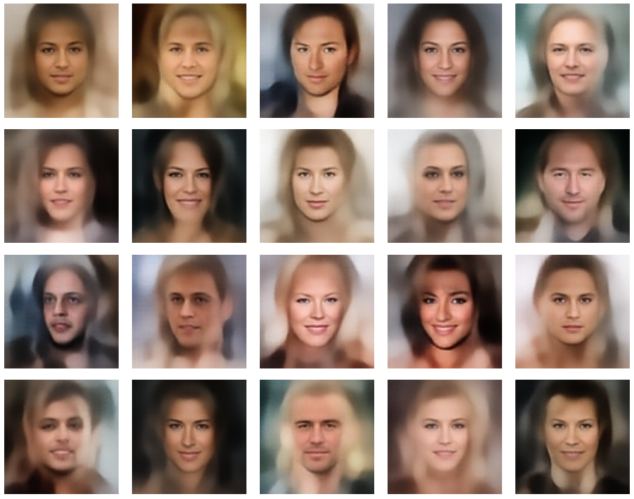
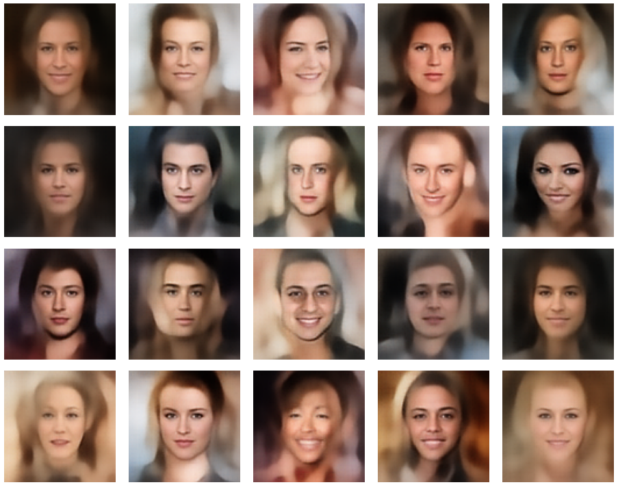
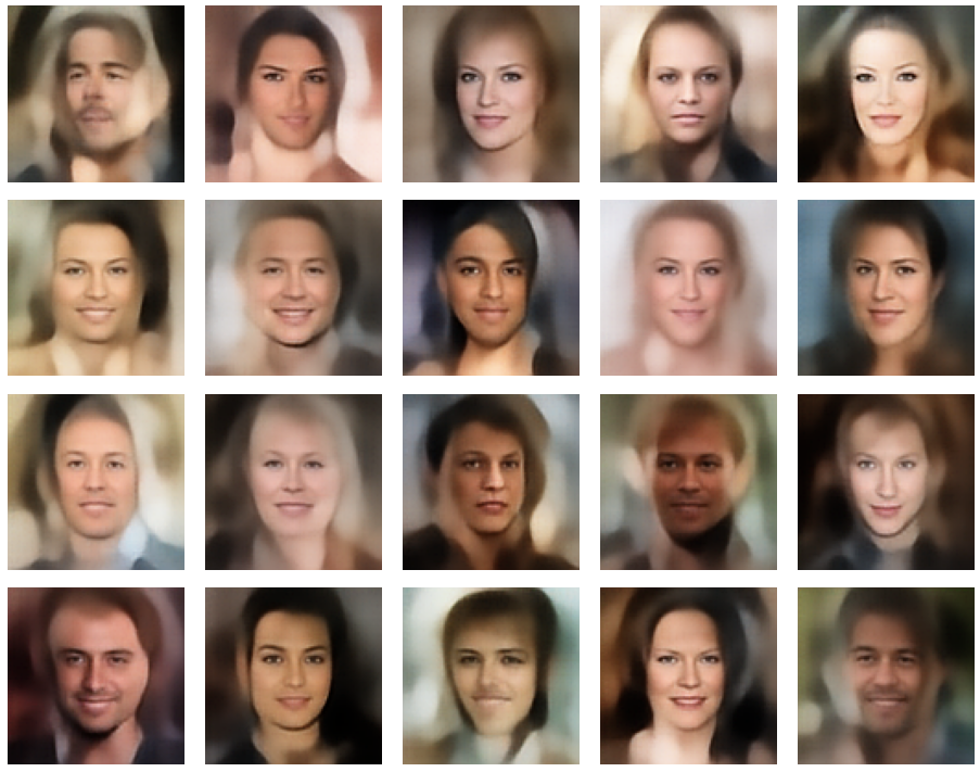
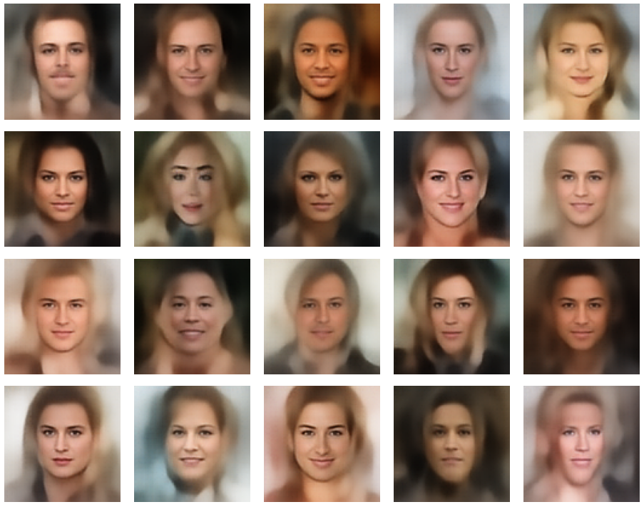
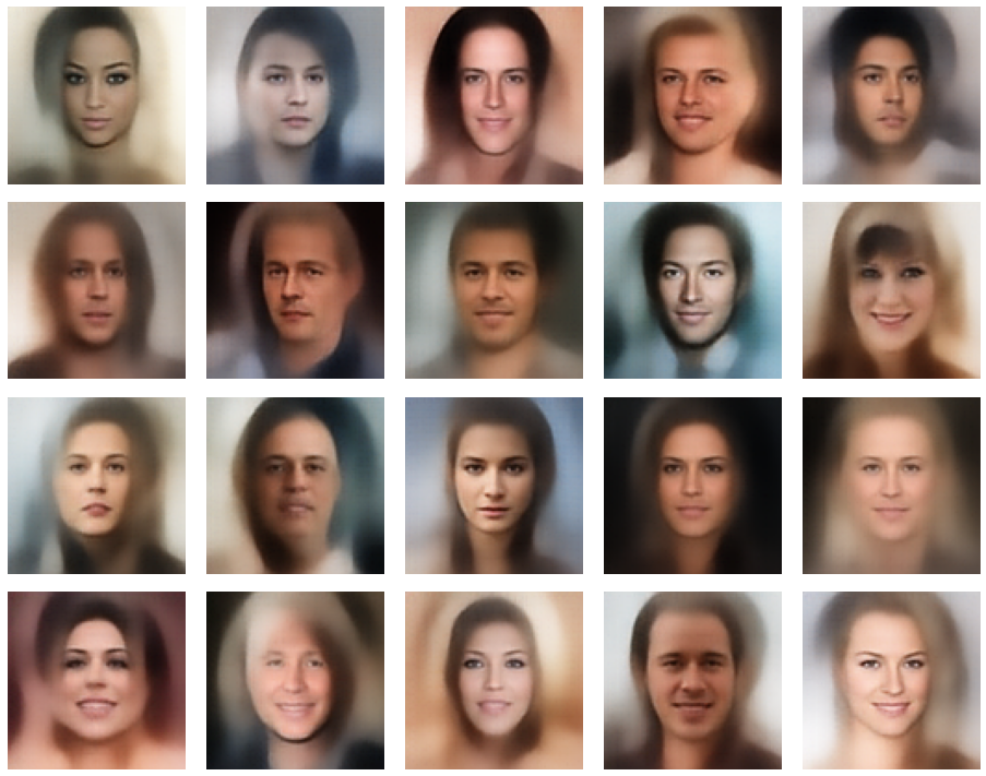
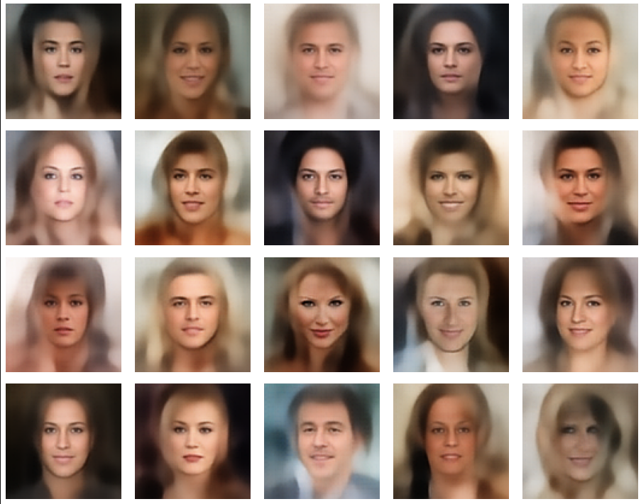
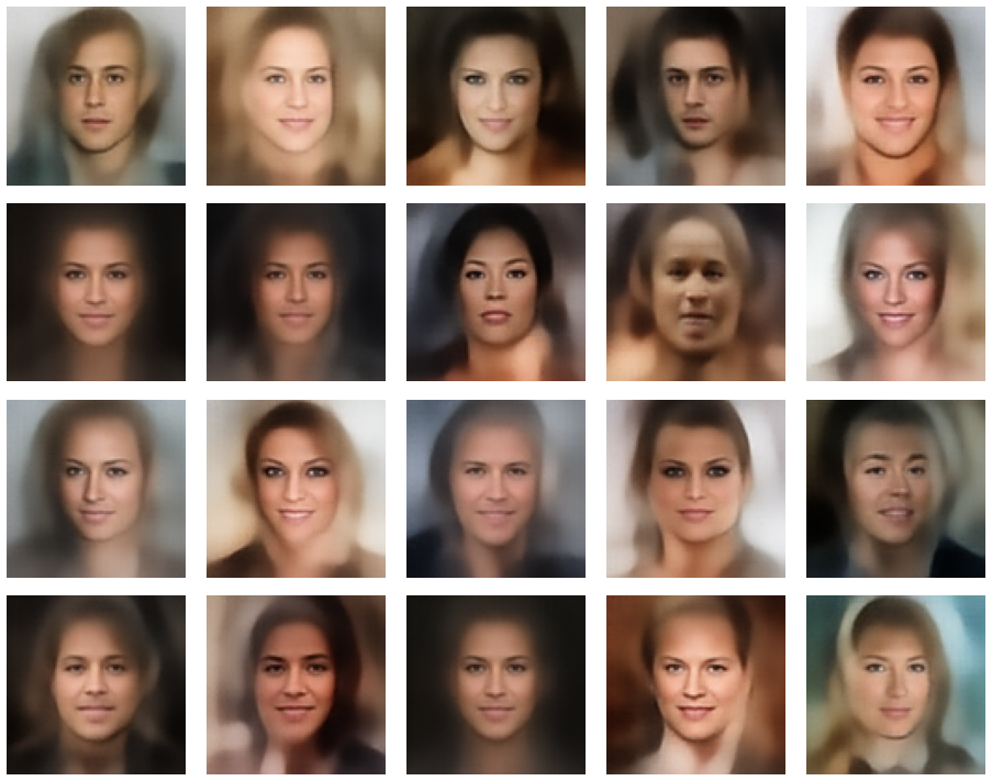
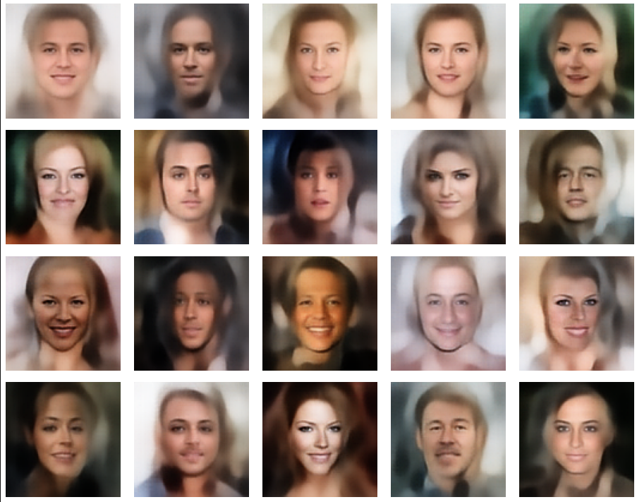
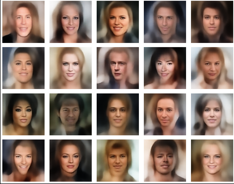
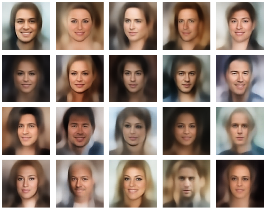
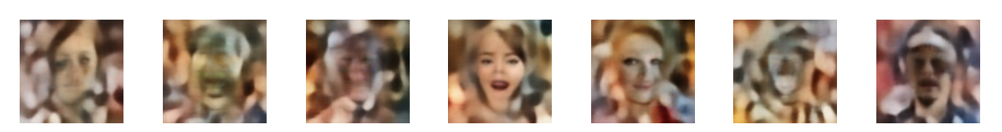
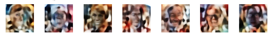
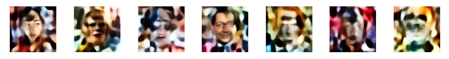
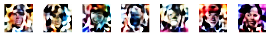
I provide the pure code of the classes in this post. In the next post you will find Jupyter cell code for an application to the Celeb A dataset. To prove that the classes below do their job in the end I show you some faces which have been created from arbitrarily chosen points in the latent space after training.

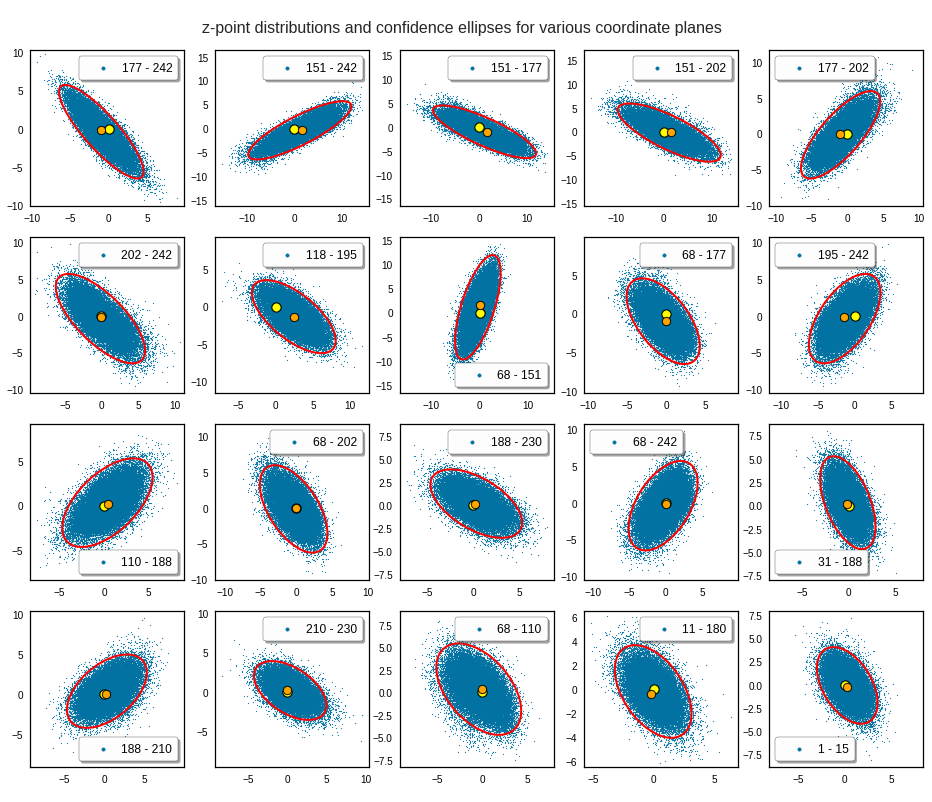
These faces do not exist in reality. They are constructed by the VAE based on compressed and “normalized” data for face patterns and face attribute distributions in the latent space. Note that I used a latent space with a dimension of z_dim =200.
Layer setup by class MyVariationalAutoencoder()
We have already many of the required methods ready. In the last posts we used the flexible functional interface of Keras to set up Neural Network models for both Encoder and Decoder, each with sequences of (convolutional) layers. For our present purposes we will not change the elementary layer structure of the Encoder or Decoder. In particular the layers for the “mu” and “log_var” contributions to the KL loss and a subsequent sampling-layer of the Encoder will remain unchanged.
In the course of the last two posts I have already introduced a parameter “solution_type” to control specifics of our VAE model. We shall use it now to invoke a child class of Keras’ Model() which allows for detailed steps of loss and gradient evaluations.
A child class of keras.models.Model() for loss and gradient evaluation
The standard Keras method Model.fit() normally provides a convenient interface for Keras users. We do not have to think about calling the low-level functions at all if we do not want to or do not need to control gradient calculations in detail. In our present approach, however, we use the low level functionality of GradientTape() directly. This requires to overwrite a specific method of the standard Keras class Model() – namely the function “train_step()”.
If you have never worked with a self-defined training_step() and GradientTape() before then I recommend to read the following introductions first:
https://www.tensorflow.org/ guide/ autodiff
customizing what happens in fit() and the relation to training_step()
These articles contain valuable information about how to operate at low level with training_step() regarding losses, derivatives and metrics. This information will help to better understand the methods of a new class VAE() which I am going to derive from Keras’ class Model() below.
Let us first briefly repeat some imports required.
Imports
# Imports
# ~~~~~~~~
import sys
import numpy as np
import os
import pickle

import tensorflow as tf
import tensorflow.keras as keras
from tensorflow.keras.layers import Layer, Input, Conv2D, Flatten, Dense, Conv2DTranspose, Reshape, Lambda, \
                                    Activation, BatchNormalization, ReLU, LeakyReLU, ELU, Dropout, AlphaDropout
from tensorflow.keras.models import Model
# to be consistent with my standard loading of the Keras backend in Jupyter notebooks:
from tensorflow.keras import backend as B
from tensorflow.keras import metrics
#from tensorflow.keras.backend import binary_crossentropy

from tensorflow.keras.optimizers import Adam
from tensorflow.keras.callbacks import ModelCheckpoint
from tensorflow.keras.utils import plot_model

#from tensorflow.python.debug.lib.check_numerics_callback import _maybe_lookup_original_input_tensor

# Personal: The following works only if the path in the notebook is supplemented by the path to /projects/GIT/mlx
# The user has to organize his paths for modules to be referred to from Jupyter notebooks himself and
# replace this settings
from mynotebooks.my_AE_code.utils.callbacks import CustomCallback, VAE_CustomCallback, step_decay_schedule
from keras.callbacks import ProgbarLogger
Now we define a class VAE() which inherits basic functionality from the Keras class Model() and overwrite the method train_step(). We shall later create an instance of this new class within an object of class MyVariationalAutoencoder().
New Class VAE
from tensorflow.keras import metrics
...
...
# A child class of Model() to control train_step with GradientTape()
class VAE(keras.Model):

    # We use our self defined __init__() to provide a reference MyVAE
    # to an object of type "MyVariationalAutoencoder"
    # This in turn allows us to address the Encoder and the Decoder
    def __init__(self, MyVAE, **kwargs):
        super(VAE, self).__init__(**kwargs)
        self.MyVAE   = MyVAE
        self.encoder = self.MyVAE.encoder
        self.decoder = self.MyVAE.decoder

        # A factor to control the ratio between the KL loss and the reconstruction loss
        self.fact = MyVAE.fact

        # A counter
        self.count = 0

        # A factor to scale the absolute values of the losses
        # e.g. by the number of pixels of an image
        self.scale_fact = 1.0  # no scaling
        # self.scale_fact = tf.constant(self.MyVAE.input_dim[0] * self.MyVAE.input_dim[1], dtype=tf.float32)
        self.f_scale    = 1. / self.scale_fact

        # loss type : 0: BCE, 1: MSE
        self.loss_type = self.MyVAE.loss_type

        # track loss development via metrics
        self.total_loss_tracker = keras.metrics.Mean(name="total_loss")
        self.reco_loss_tracker  = keras.metrics.Mean(name="reco_loss")
        self.kl_loss_tracker    = keras.metrics.Mean(name="kl_loss")

    def call(self, inputs):
        x, z_m, z_var = self.encoder(inputs)
        return self.decoder(x)

    # Overwrite the metrics() of Model() - use getter mechanism
    @property
    def metrics(self):
        return [
            self.total_loss_tracker,
            self.reco_loss_tracker,
            self.kl_loss_tracker
        ]

    # Core function to control all operations regarding eager differentiation operations,
    # i.e. the calculation of loss terms with respect to tensors and differentiation variables
    # and metrics data
    def train_step(self, data):
        # We use the GradientTape context to record differntiation operations/results
        #self.count += 1

        with tf.GradientTape() as tape:
            z, z_mean, z_log_var = self.encoder(data)
            reconstruction = self.decoder(z)
            #reco_shape = tf.shape(self.reconstruction)
            #print("reco_shape = ", reco_shape, self.reconstruction.shape, data.shape)

            #BCE loss (Binary Cross Entropy)
            if self.loss_type == 0:
                reconstruction_loss = tf.reduce_mean(
                    tf.reduce_sum(
                        keras.losses.binary_crossentropy(data, reconstruction), axis=(1, 2)
                    )
                ) * self.f_scale

            # MSE loss (Mean Squared Error)
            if self.loss_type == 1:
                reconstruction_loss = tf.reduce_mean(
                    tf.reduce_sum(
                        keras.losses.mse(data, reconstruction), axis=(1, 2)
                    )
                ) * self.f_scale

            kl_loss = -0.5 * self.fact * (1 + z_log_var - tf.square(z_mean) - tf.exp(z_log_var))
            kl_loss = tf.reduce_mean(tf.reduce_sum(kl_loss, axis=1))
            total_loss = reconstruction_loss + kl_loss

        grads = tape.gradient(total_loss, self.trainable_weights)
        self.optimizer.apply_gradients(zip(grads, self.trainable_weights))
        #if self.count == 1:

        self.total_loss_tracker.update_state(total_loss)
        self.reco_loss_tracker.update_state(reconstruction_loss)
        self.kl_loss_tracker.update_state(kl_loss)
        return {
            "total_loss": self.total_loss_tracker.result(),
            "reco_loss": self.reco_loss_tracker.result(),
            "kl_loss": self.kl_loss_tracker.result(),
        }

    def compile_VAE(self, learning_rate):

        # Optimizer
        # ~~~~~~~~~
        optimizer = Adam(learning_rate=learning_rate)
        # save the learning rate for possible intermediate output to files
        self.learning_rate = learning_rate
        self.compile(optimizer=optimizer)
Explanation of class VAE(): Details of the methods of the additional class
First, we need to import an additional library tensorflow.keras.metrics. Its functions, as e.g. Mean(), will help us to print out intermediate data about various loss contributions during training – averaged over the batches of an epoch.
Then, we have added four central methods to class VAE:
- a function __init__(),
- a function metrics() together with Python’s getter-mechanism
- a function call()
- and our central function training_step().
All functions overwrite the defaults of the parent class Model(). Be careful to distinguish the range of batches which keras.metrics() and training_step() operate on:
- A “training step” covers just one batch eventually provided to the training mechanism by the Model.fit()-function.
- Averaging performed by functions of keras.metrics instead works across all batches of an epoch.
Functions “__init__() ” and call() to instantiate a Model based on class VAE()
In general we can use the standard interface of __init__(inputs, outputs, …) or a call()-interface to instantiate an object of class-type Model(). See
https://www.tensorflow.org/ api_docs/python/ tf/ keras/ Model
https://docs.w3cub.com/ tensorflow~python/ tf/ keras/ model.html
We have to be precise about the parameters of __init()__ or the call()-interface if we intend to use properties of the standard compile()– and fit()-interfaces of a model – at least in application cases where we do not control everything regarding losses and gradients ourselves.
To define a complete model for the general case we therefore add the call()-method. At the same time we “misuse” the __init__() function of VAE() to provide a reference to our instance of class “MyVariationalAutoencoder”. Actually, providing “call()” is done only for the sake of flexibility in other use cases than the one discussed here. For our present purposes we could actually omit call().
The __init__()-function retrieves some parameters from MyVAE. You see the factor “fact” which controls the ratio of the KL-loss to the reconstruction loss. In addition I provided an option to scale the loss values by a division by the number of pixels of input images. You just have to un-comment the respective statement. Sorry, I have not yet made it controllable by a parameter of MyVariationalAutoencoder().
Finally, the parameter loss_type is evaluated; for a value of “1” we take MSE as a loss function instead of the standard BCE (Binary Cross-Entropy); see the Jupyter cells in the next post. This allows for some more flexibility in dealing with certain datasets.
Function “metrics()” to produce loss values as output during training
With the function metrics() we are able to establish our own “tracking” of the evolution of the Model’s loss contributions during training. In our case we are particularly interested in the evolution of the “reconstruction loss” and the “KL-loss“.
Note that the @property decorator is added to the metrics()-function. This allows us to define its output via the getter-mechanism for Python classes. In our case the __init__()-function defines the mechanism to fill required variables:
The three “tracker”-variables there get their values from the function tensorflow.keras.metrics.Mean(). Note that the names given to the loss-trackers in __init__() are of importance for later output handling!
Note also that keras.metrics.Mean() calculates averages over values derived for all batches of an epoch. The tf.reduce_mean()-statements in the GradientTape() section of the code above, instead, refer to averages calculated over the samples of a single batch.
Actualized loss output is later delivered during each training step by the method update_state(). You find a description of the methods of keras.metrics.Mean() here.
The result of all this is that metrics() delivers loss values by actualized tracker-variables of our child class VAE(). Note that neither __init__() nor metrics() define what exactly is to be done to calculate each loss term. __init__() and metrics() only prepare the later output technically by formal class constructs. Note also that all the data defined by metrics() are updated and averaged per epoch without the requirement to call the function “reset_states()” (see the Keras docs). This is automatically done at the beginning of each epoch.
train_step() and GradientTape() to control losses and their gradients
Let us turn to the necessary calculations which must be performed during each training step. In an eager environment we must watch the trainable variables, on which the different loss terms depend, to be able to calculate the partial derivatives and record related operations and intermediate results already during forward pass:
We must track the differentiation operations and resulting values to know exactly what has to be done in reverse during error backward propagation. To be able to do this TF2 offers us a recording mechanism called GradientTape(). Its results are kept in an object which often is called a “tape”.
You find more information about these topics at
https://debuggercafe.com/ basics-of-tensorflow-gradienttape/
https://runebook.dev/de/docs/ tensorflow/gradienttape
Within train_step() we need some tensors which are required for loss calculations in an explicit form. So, we must change the Keras model for the Encoder to give us the tensors for “mu” and “log_var” as its output.
This is no problem for us. We have already made the output of the Encoder dependent on a variable “solution_type” and discussed a multi-output Encoder model already in the post Variational Autoencoder with Tensorflow 2.8 – VI – KL loss via tensor transfer and multiple output.
Therefore, we just have to add a new value 3 to the checks of “solution_type”. The same is true for the input control of the Decoder (see a section about the related methods of MyVariationalAutoencoder() below).
The statements within the section for GradientTape() deal with the calculation of loss terms and record the related operations. All the calculations should be be familiar from previous posts of this series.
This includes an identification of the trainable_weights of the involved layers. Quote from
https://keras.io/ guides/ writing_a_ training_loop_ from_scratch/ #using-the-gradienttape-a-first-endtoend-example:
Calling a model inside a GradientTape scope enables you to retrieve the gradients of the trainable weights of the layer with respect to a loss value. Using an optimizer instance, you can use these gradients to update these variables (which you can retrieve using model.trainable_weights).
In train_step() we need to register that the total loss is dependent on all trainable weights and that all related partial derivatives have to be taken into account during optimization. This is done by
        grads = tape.gradient(total_loss, self.trainable_weights)
        self.optimizer.apply_gradients(zip(grads, self.trainable_weights))
To be able to get actualized output during training we update the state of all tracked variables:
        self.total_loss_tracker.update_state(total_loss)
        self.reco_loss_tracker.update_state(reco_loss)
        self.kl_loss_tracker.update_state(kl_loss)
A small problem with F. Chollet’s code
The careful reader may have noticed that my code of the function “train_step()” deviates from F. Chollet’s recommendations. Regarding the return statement I use
        return {
            "total_loss": self.total_loss_tracker.result(),
            "reco_loss": self.reco_loss_tracker.result(),
            "kl_loss": self.kl_loss_tracker.result(),
        }
whilst F. Chollet’s original code contains a statement like
        return {
            "loss": self.total_loss_tracker.result(),     # here lies the main difference - different "name" than defined in __init__!
            "reconstruction_loss": self.reconstruction_loss_tracker.result(),  # ignore my abbreviation to reco_loss
            "kl_loss": self.kl_loss_tracker.result(),
        }
Chollet’s original code unfortunately gives inconsistent loss data: The sum of his “reconstruction loss” and the “KL (Kullback Leibler) loss” do not add up to the (total) “loss”. This can be seen from the data of the first epochs in F. Chollet’s example on the tutorial at
keras.io/ examples/ generative/ vae.
Some of my own result data for the MNIST example with this error look like:
Epoch 1/5
469/469 [============================_build_dec==] - 7s 13ms/step - reconstruction_loss: 209.0115 - kl_loss: 3.4888 - loss: 258.9048
Epoch 2/5
469/469 [==============================] - 7s 14ms/step - reconstruction_loss: 173.7905 - kl_loss: 4.8220 - loss: 185.0963
Epoch 3/5
469/469 [==============================] - 6s 13ms/step - reconstruction_loss: 160.4016 - kl_loss: 5.7511 - loss: 167.3470
Epoch 4/5
469/469 [==============================] - 6s 13ms/step - reconstruction_loss: 155.5937 - kl_loss: 5.9947 - loss: 162.3994
Epoch 5/5
469/469 [==============================] - 6s 13ms/step - reconstruction_loss: 152.8330 - kl_loss: 6.1689 - loss: 159.5607
Things do get better from epoch to epoch – but we want a consistent output from the beginning: The averaged (total) loss should always be printed as equal to the sum of the averaged) KL loss plus the reconstruction loss.
The deviation is surprising as we seem to use the right tracker-results in the code. And the name used in the return statement of the train_step()-function here should only be relevant for the printing …
However, the name “loss” is NOT consistent with the name defined in the statement Mean(name=”total_loss”) in the __init__() function of Chollet, where he defines his tracking mechanisms.
self.total_loss_tracker = keras.metrics.Mean(name="total_loss")
This has consequences: The inconsistency triggers a different output than a consistent use of names. Just try it out on your own …
This is not only true for the deviation between “loss” in
return {
            "loss": self.total_loss_tracker.result(),
            ....
       }
and “total_loss” in the __init__) function
self.total_loss_tracker = keras.metrics.Mean(name="total_loss") , namely a value lacking averaging -
but also for deviations in the names used for the other loss contributions. In case of an inconsistency Keras seems to fall back to a default here which does not reflect the standard linear averaging of Mean() over all values calculated for the batches of an epoch (without any special weights).
That there is some common default mechanism working can be seen from the fact that wrong names for all individual losses (here the KL loss and the reconstruction loss) give us at least a consistent sum-value for the total amount again. But all the values derived by the fallback are much closer to the start values at an epochs begin than the mean values averaged over an epoch. You may test this yourself.
To get on the safe side we use the correct “names” defined in the __init__()-function of our code:
        return {
            "total_loss": self.total_loss_tracker.result(),
            "reco_loss": self.reco_loss_tracker.result(),
            "kl_loss": self.kl_loss_tracker.result(),
        }
For MNIST data fed into our VAE model we then get:
Epoch 1/5
469/469 [==============================] - 8s 13ms/step - reco_loss: 214.5662 - kl_loss: 2.6004 - total_loss: 217.1666
Epoch 2/5
469/469 [==============================] - 7s 14ms/step - reco_loss: 186.4745 - kl_loss: 3.2799 - total_loss: 189.7544
Epoch 3/5
469/469 [==============================] - 6s 13ms/step - reco_loss: 181.9590 - kl_loss: 3.4186 - total_loss: 185.3774
Epoch 4/5
469/469 [==============================] - 6s 13ms/step - reco_loss: 177.5216 - kl_loss: 3.9433 - total_loss: 181.4649
Epoch 5/5
469/469 [==============================] - 6s 13ms/step - reco_loss: 163.7209 - kl_loss: 5.5816 - total_loss: 169.3026
This is exactly what we want.
A general recipe to use train_step()
So, the general recipe is:
- Define what metric properties you are interested in. Create respective tracker-variables in the __init__() function.
- Use the getter mechanism to define your metrics() function and its output via references to the trackers.
- Define your own training step by a function train_step().
- Use Tensorflow’s GradientTape context to register statements which control the calculation of loss contributions from elementary tensors of your (functional) Keras model. Provide all layers there, e.g. by references to their models.
- Register gradient-operations of the total loss with respect to all trainable weights and updates of metrics data within function “train_step()”.
Actually, I have used the GradientTape() mechanism already in this blog when I played a bit with approaches to create so called DeepDream images. See
https://linux-blog.anracom.com/category/machine-learning/deep-dream/
for more information – there in a different context.
How to combine the classes “VAE()” and “MyVariationalAutoencoder()” ?
Where do we stand? We have defined a new class “VAE()” which modifies the original Keras Model() class. And we have our class “MyVariationalAutoencoder()” to control the setup of a VAE model.
Next we need to address the question of how we combine these two classes. If you have read my previous posts you may expect a major change to the method “_build_VAE()“. This is correct, but we also have to modify the conditions for the Encoder output construction in _build_enc() and the definition of the Decoder’s input in _build_dec(). Therefore I give you the modified code for these functions. For reasons of completeness I add the code for the __init__()-function:
Function __init__()
    def __init__(self
        , input_dim                  # the shape of the input tensors (for MNIST (28,28,1))
        , encoder_conv_filters       # number of maps of the different Conv2D layers
        , encoder_conv_kernel_size   # kernel sizes of the Conv2D layers
        , encoder_conv_strides       # strides - here also used to reduce spatial resolution avoid pooling layers
                                     # used instead of Pooling layers
        , encoder_conv_padding       # padding - valid or same

        , decoder_conv_t_filters     # number of maps in Con2DTranspose layers
        , decoder_conv_t_kernel_size # kernel sizes of Conv2D Transpose layers
        , decoder_conv_t_strides     # strides for Conv2dTranspose layers - inverts spatial resolution
        , decoder_conv_t_padding     # padding - valid or same

        , z_dim                      # A good start is 16 or 24
        , solution_type  = 0         # Which type of solution for the KL loss calculation ?
        , act            = 0         # Which type of activation function?
        , fact           = 0.65e-4   # Factor for the KL loss (0.5e-4 < fact < 1.e-3is reasonable)
        , loss_type      = 0         # 0: BCE, 1: MSE
        , use_batch_norm = False     # Shall BatchNormalization be used after Conv2D layers?
        , use_dropout    = False     # Shall statistical dropout layers be used for tregularization purposes ?
        , dropout_rate   = 0.25      # Rate for statistical dropout layer
        , b_build_all    = False     # Added by RMO - full Model is build in 2 steps
        ):

        '''
        Input:
        The encoder_... and decoder_.... variables are Python lists,
        whose length defines the number of Conv2D and Conv2DTranspose layers

        input_dim : Shape/dimensions of the input tensor - for MNIST (28,28,1)
        encoder_conv_filters:     List with the number of maps/filters per Conv2D layer
        encoder_conv_kernel_size: List with the kernel sizes for the Conv-Layers
        encoder_conv_strides:     List with the strides used for the Conv-Layers

        z_dim : dimension of the "latent_space"
        solution_type : Type of solution for KL loss calculation (0: Customized Encoder layer,
                                                                  1: transfer of mu, var_log to Decoder
                                                                  2: model.add_loss()
                                                                  3: definition of training step with Gradient.Tape()

        act :  determines activation function to use (0: LeakyRELU, 1:RELU , 2: SELU)
               !!!! NOTE: !!!!
               If SELU is used then the weight kernel initialization and the dropout layer need to be special
               https://github.com/christianversloot/machine-learning-articles/blob/main/using-selu-with-tensorflow-and-keras.md
               AlphaDropout instead of Dropout + LeCunNormal for kernel initializer
        fact = 0.65e-4 : Factor to scale the KL loss relative to the reconstruction loss
                         Must be adapted to the way of calculation -
                         e.g. for solution_type == 3 the loss is not averaged over all pixels
                         => at least factor of around 1000 bigger than normally
        loss-type = 0:   Defines the way we calculate a reconstruction loss
                         0: Binary Cross Entropy - recommended by many authors
                         1: Mean Square error - recommended by some authors especially for "face arithmetics"
        use_batch_norm = False   # True : We use BatchNormalization
        use_dropout    = False   # True : We use dropout layers (rate = 0.25, see Encoder)
        b_build_all    = False   # True : Full VAE Model is build in 1 step;
                                   False: Encoder, Decoder, VAE are build in separate steps
        '''

        self.name = 'variational_autoencoder'

        # Parameters for Layers which define the Encoder and Decoder
        self.input_dim                  = input_dim
        self.encoder_conv_filters       = encoder_conv_filters
        self.encoder_conv_kernel_size   = encoder_conv_kernel_size
        self.encoder_conv_strides       = encoder_conv_strides
        self.encoder_conv_padding       = encoder_conv_padding

        self.decoder_conv_t_filters     = decoder_conv_t_filters
        self.decoder_conv_t_kernel_size = decoder_conv_t_kernel_size
        self.decoder_conv_t_strides     = decoder_conv_t_strides
        self.decoder_conv_t_padding     = decoder_conv_t_padding

        self.z_dim = z_dim

        # Check param for activation function
        if act < 0 or act > 2:
            print("Range error: Parameter act = " + str(act) + " has unknown value ")
            sys.exit()
        else:
            self.act = act

        # Factor to scale the KL loss relative to the Binary Cross Entropy loss
        self.fact = fact

        # Type of loss - 0: BCE, 1: MSE
        self.loss_type = loss_type


        # Check param for solution approach
        if solution_type < 0 or solution_type > 3:
            print("Range error: Parameter solution_type = " + str(solution_type) + " has unknown value ")
            sys.exit()
        else:
            self.solution_type = solution_type

        self.use_batch_norm = use_batch_norm
        self.use_dropout    = use_dropout
        self.dropout_rate   = dropout_rate

        # Preparation of some variables to be filled later
        self._encoder_input  = None  # receives the Keras object for the Input Layer of the Encoder
        self._encoder_output = None  # receives the Keras object for the Output Layer of the Encoder
        self.shape_before_flattening = None # info of the Encoder => is used by Decoder
        self._decoder_input  = None  # receives the Keras object for the Input Layer of the Decoder
        self._decoder_output = None  # receives the Keras object for the Output Layer of the Decoder

        # Layers / tensors for KL loss
        self.mu      = None # receives special Dense Layer's tensor for KL-loss
        self.log_var = None # receives special Dense Layer's tensor for KL-loss

        # Parameters for SELU - just in case we may need to use it somewhere
        # https://keras.io/api/layers/activations/ see selu
        self.selu_scale = 1.05070098
        self.selu_alpha = 1.67326324

        # The number of Conv2D and Conv2DTranspose layers for the Encoder / Decoder
        self.n_layers_encoder = len(encoder_conv_filters)
        self.n_layers_decoder = len(decoder_conv_t_filters)

        self.num_epoch = 0 # Intialization of the number of epochs

        # A matrix for the values of the losses
        self.std_loss  = tf.TensorArray(tf.float32, size=0, dynamic_size=True, clear_after_read=False)

        # We only build the whole AE-model if requested
        self.b_build_all = b_build_all
        if b_build_all:
            self._build_all()
Changes to the Encoder and Decoder code
We just need to set the right options for the output tensors of the Encoder and the input tensors of the Decoder. The relevant code parts are controlled by the parameter “solution_type”.
Modified code of _build_enc() of class MyVariationalAutoencoder
    def _build_enc(self, solution_type = -1, fact=-1.0):
        '''  Your documentation '''
        # Checking whether "fact" and "solution_type" for the KL loss shall be overwritten
        if fact < 0:
            fact = self.fact
        if solution_type < 0:
            solution_type = self.solution_type
        else:
            self.solution_type = solution_type

        # Preparation: We later need a function to calculate the z-points in the latent space
        # The following function wiChangedll be used by an eventual Lambda layer of the Encoder
        def z_point_sampling(args):
            '''
            A point in the latent space is calculated statistically
            around an optimized mu for each sample
            '''
            mu, log_var = args # Note: These are 1D tensors !
            epsilon = B.random_normal(shape=B.shape(mu), mean=0., stddev=1.)
            return mu + B.exp(log_var / 2) * epsilon


        # Input "layer"
        self._encoder_input = Input(shape=self.input_dim, name='encoder_input')

        # Initialization of a running variable x for individual layers
        x = self._encoder_input

        # Build the CNN-part with Conv2D layers
        # Note that stride>=2 reduces spatial resolution without the help of pooling layers
        for i in range(self.n_layers_encoder):
            conv_layer = Conv2D(
                filters = self.encoder_conv_filters[i]
                , kernel_size = self.encoder_conv_kernel_size[i]
                , strides = self.encoder_conv_strides[i]
                , padding = 'same'  # Important ! Controls the shape of the layer tensors.
                , name = 'encoder_conv_' + str(i)
                )
            x = conv_layer(x)

            # The "normalization" should be done ahead of the "activation"
            if self.use_batch_norm:
                x = BatchNormalization()(x)

            # Selection of activation function (out of 3)
            if self.act == 0:
                x = LeakyReLU()(x)
            elif self.act == 1:
                x = ReLU()(x)
            elif self.act == 2:
                # RMO: Just use the Activation layer to use SELU with predefined (!) parameters
                x = Activation('selu')(x)

            # Fulfill some SELU requirements
            if self.use_dropout:
                if self.act == 2:
                    x = AlphaDropout(rate = 0.25)(x)
                else:
                    x = Dropout(rate = 0.25)(x)

        # Last multi-dim tensor shape - is later needed by the decoder
        self._shape_before_flattening = B.int_shape(x)[1:]

        # Flattened layer before calculating VAE-output (z-points) via 2 special layers
        x = Flatten()(x)

        # "Variational" part - create 2 Dense layers for a statistical distribution of z-points
        self.mu      = Dense(self.z_dim, name='mu')(x)
        self.log_var = Dense(self.z_dim, name='log_var')(x)

        if solution_type == 0:
            # Customized layer for the calculation of the KL loss based on mu, var_log data
            # We use a customized layer according to a class definition
            self.mu, self.log_var = My_KL_Layer()([self.mu, self.log_var], fact=fact)


        # Layer to provide a z_point in the Latent Space for each sample of the batch
        self._encoder_output = Lambda(z_point_sampling, name='encoder_output')([self.mu, self.log_var])

        # The Encoder Model
        # ~~~~~~~~~~~~~~~~~~~
        # With extra KL layer or with vae.add_loss()
        if self.solution_type == 0 or self.solution_type == 2:
            self.encoder = Model(self._encoder_input, self._encoder_output, name="encoder")

        # Transfer solution => Multiple outputs
        if self.solution_type == 1  or self.solution_type == 3:
            self.encoder = Model(inputs=self._encoder_input, outputs=[self._encoder_output, self.mu, self.log_var], name="encoder")
The difference is the dependency of the output on “solution_type 3”. For the Decoder we have:
Modified code of _build_enc() of class MyVariationalAutoencoder
    def _build_dec(self):
        ''' Your documentation       '''

        # Input layer - aligned to the shape of z-points in the latent space = output[0] of the Encoder
        self._decoder_inp_z = Input(shape=(self.z_dim,), name='decoder_input')

        # Additional Input layers for the KL tensors (mu, log_var) from the Encoder
        if self.solution_type == 1  or self.solution_type == 3:
            self._dec_inp_mu       = Input(shape=(self.z_dim), name='mu_input')
            self._dec_inp_var_log  = Input(shape=(self.z_dim), name='logvar_input')

            # We give the layers later used as output a name
            # Each of the Activation layers below just correspond to an identity passed through
            #self._dec_mu            = self._dec_inp_mu
            #self._dec_var_log       = self._dec_inp_var_log
            self._dec_mu            = Activation('linear',name='dc_mu')(self._dec_inp_mu)
            self._dec_var_log       = Activation('linear', name='dc_var')(self._dec_inp_var_log)

        # Here we use the tensor shape info from the Encoder
        x = Dense(np.prod(self._shape_before_flattening))(self._decoder_inp_z)
        x = Reshape(self._shape_before_flattening)(x)

        # The inverse CNN
        for i in range(self.n_layers_decoder):
            conv_t_layer = Conv2DTranspose(
                filters = self.decoder_conv_t_filters[i]
                , kernel_size = self.decoder_conv_t_kernel_size[i]
                , strides = self.decoder_conv_t_strides[i]
                , padding = 'same' # Important ! Controls the shape of tensors during reconstruction
                                   # we want an image with the same resolution as the original input
                , name = 'decoder_conv_t_' + str(i)
                )
            x = conv_t_layer(x)

            # Normalization and Activation
            if i < self.n_layers_decoder - 1:
                # Also in the decoder: normalization before activation
                if self.use_batch_norm:
                    x = BatchNormalization()(x)

                # Choice of activation function
                if self.act == 0:
                    x = LeakyReLU()(x)
                elif self.act == 1:
                    x = ReLU()(x)
                elif self.act == 2:
                    #x = self.selu_scale * ELU(alpha=self.selu_alpha)(x)
                    x = Activation('selu')(x)

                # Adaptions to SELU requirements
                if self.use_dropout:
                    if self.act == 2:
                        x = AlphaDropout(rate = 0.25)(x)
                    else:
                        x = Dropout(rate = 0.25)(x)

            # Last layer => Sigmoid output
            # => This requires s<pre style="padding:8px; height: 400px; overflow:auto;">caled input => Division of pixel values by 255
            else:
                x = Activation('sigmoid', name='dc_reco')(x)

        # Output tensor => a scaled image
        self._decoder_output = x

        # The Decoder model
        # solution_type == 0/2/3: Just the decoded input
        if self.solution_type == 0 or self.solution_type == 2 or self.solution_type == 3:
            self.decoder = Model(self._decoder_inp_z, self._decoder_output, name="decoder")

        # solution_type == 1: The decoded tensor plus the transferred tensors mu and log_var a for the variational distribution
        if self.solution_type == 1:
            self.decoder = Model([self._decoder_inp_z, self._dec_inp_mu, self._dec_inp_var_log],
                                 [self._decoder_output, self._dec_mu, self._dec_var_log], name="decoder")
Changes to the methods _build_VAE for building the VAE model
Our VAE model now is set up with the help of the __init__() method of our new class VAE. We just have to supplement the object created by MyVariationalAutoencoder.
Modified code of _build_VAE() of class MyVariationalAutoencoder
    def _build_VAE(self):
        ''' Your documentation '''

        # Solution with train_step() and GradientTape(): Control is transferred to class VAE
        if self.solution_type == 3:
            self.model = VAE(self)   # Here parameter "self" provides a reference to an instance of MyVariationalAutoencoder
            self.model.summary()

        # Solutions with layer.add_loss or model.add_loss()
        if self.solution_type == 0 or self.solution_type == 2:
            model_input  = self._encoder_input
            model_output = self.decoder(self._encoder_output)
            self.model = Model(model_input, model_output, name="vae")

        # Solution with transfer of data from the Encoder to the Decoder output layer
        if self.solution_type == 1:
            enc_out      = self.encoder(self._encoder_input)
            dc_reco, dc_mu, dc_var = self.decoder(enc_out)
            # We organize the output and later association of cost functions and metrics via a dictionary
            mod_outputs = {'vae_out_main': dc_reco, 'vae_out_mu': dc_mu, 'vae_out_var': dc_var}
            self.model = Model(inputs=self._encoder_input, outputs=mod_outputs, name="vae")
Note that we keep the resulting model within the object for class MyVariationalAutoencoder. See the Jupyter cells in my next post.
Changes to the method compile_myVAE()
The modification of the function compile_myVAE is simple
    def compile_myVAE(self, learning_rate):

        # Optimizer
        # ~~~~~~~~~
        optimizer = Adam(learning_rate=learning_rate)
        # save the learning rate for possible intermediate output to files
        self.learning_rate = learning_rate

        # Parameter "fact" will be used by the cost functions defined below to scale the KL loss relative to the BCE loss
        fact = self.fact

        # Function for solution_type == 1
        # ~~~~~~~~~~~~~~~~~~~~~~~~~~~~~~~~~
        @tf.function
        def mu_loss(y_true, y_pred):
            loss_mux = fact * tf.reduce_mean(tf.square(y_pred))
            return loss_mux

        @tf.function
        def logvar_loss(y_true, y_pred):
            loss_varx = -fact * tf.reduce_mean(1 + y_pred - tf.exp(y_pred))
            return loss_varx

        # Function for solution_type == 2
        # ~~~~~~~~~~~~~~~~~~~~~~~~~~~~~~~~
        # We follow an approach described at
        # https://www.tensorflow.org/api_docs/python/tf/keras/layers/Layer
        # NOTE: We can NOT use @tf.function here
        def get_kl_loss(mu, log_var):
            kl_loss = -fact * tf.reduce_mean(1 + log_var - tf.square(mu) - tf.exp(log_var))
            return kl_loss


        # Required operations for solution_type==2 => model.add_loss()
        # ~~~~~~~~~~~~~~~~~~~~~~~~~~~~~~~~~~~~~~~~~
        res_kl = get_kl_loss(mu=self.mu, log_var=self.log_var)

        if self.solution_type == 2:
            self.model.add_loss(res_kl)
            self.model.add_metric(res_kl, name='kl', aggregation='mean')

        # Model compilation
        # ~~~~~~~~~~~~~~~~~~~~

        # Solutions with layer.add_loss or model.add_loss()
        if self.solution_type == 0 or self.solution_type == 2:
            if self.loss_type == 0:
                self.model.compile(optimizer=optimizer, loss="binary_crossentropy",
                                   metrics=[tf.keras.metrics.BinaryCrossentropy(name='bce')])
            if self.loss_type == 1:
                self.model.compile(optimizer=optimizer, loss="mse",
                                   metrics=[tf.keras.metrics.MSE(name='mse')])

        # Solution with transfer of data from the Encoder to the Decoder output layer
        if self.solution_type == 1:
            if self.loss_type == 0:
                self.model.compile(optimizer=optimizer
                                   , loss={'vae_out_main':'binary_crossentropy', 'vae_out_mu':mu_loss, 'vae_out_var':logvar_loss}
                                   #, metrics={'vae_out_main':tf.keras.metrics.BinaryCrossentropy(name='bce'), 'vae_out_mu':mu_loss, 'vae_out_var': logvar_loss }
                                   )
            if self.loss_type == 1:
                self.model.compile(optimizer=optimizer
                                   , loss={'vae_out_main':'mse', 'vae_out_mu':mu_loss, 'vae_out_var':logvar_loss}
                                   #, metrics={'vae_out_main':tf.keras.metrics.MSE(name='mse'), 'vae_out_mu':mu_loss, 'vae_out_var': logvar_loss }
                                   )

        # Solution with train_step() and GradientTape(): Control is transferred to class VAE
        if self.solution_type == 3:
            self.model.compile(optimizer=optimizer)
Note the adaptions to the new parameter “loss_type” which we have added to the __init__()-function!
Changes to the method train_myVAE() – inclusion of a dataflow “generator“
It gets a bit more complicated for the function “train_myVAE()”. The reason is that we use the opportunity to include the output of so called generators which create limited batches on the fly from disc or memory.
Such a generator is very useful if you have to handle datasets which you cannot get into the VRAM of your video card. A typical case might be the Celeb A dataset for older graphics cards as mine.
In such a case we provide a dataflow to the function. The batches in this data flow are continuously created as needed and handed over to Tensorflows data processing on the graphics card. So, “x_train” as an input variable must not be taken literally in this case! It is replaced by the generator’s dataflow then. See the code for the Jupyter cells in the next post.
In addition we prepare for cases where we have to provide target data to compare the input data “x_train” to which deviate from each other. Typical cases are the application of AEs/VAEs for denoising or recolorization.
    # Function to initiate training
    # ~~~~~~~~~~~~~~~~~~~~~~~~~~~~~~~~
    def train_myVAE(self, x_train, x_target=None
                    , b_use_generator   = False
                    , b_target_ne_train = False
                    , batch_size = 32
                    , epochs = 2
                    , initial_epoch = 0,
                    t_mu=None,
                    t_logvar=None
                    ):

        '''
        @note: Sometimes x_target MUST be provided - e.g. for Denoising, Recolorization
        @note: x_train will come as a dataflow in case of a generator
        '''

        # cax = ProgbarLogger(count_mode='samples', stateful_metrics=None)

        class MyPrinterCallback(tf.keras.callbacks.Callback):
            # def on_train_batch_begin(self, batch, logs=None):
            #     # Do something on begin of training batch

            def on_epoch_end(self, epoch, logs=None):
                # Get overview over available keys
                #keys = list(logs.keys())
                print("\nEPOCH: {}, Total Loss: {:8.6f}, // reco loss: {:8.6f}, mu Loss: {:8.6f}, logvar loss: {:8.6f}".format(epoch,
                      logs['loss'], logs['decoder_loss'], logs['decoder_1_loss'], logs['decoder_2_loss']
                                            ))
                print()
                #print('EPOCH: {}, Total Loss: {}'.format(epoch, logs['loss']))
                #print('EPOCH: {}, metrics: {}'.format(epoch, logs['metrics']))

            def on_epoch_begin(self, epoch, logs=None):
                print('-'*50)
                print('STARTING EPOCH: {}'.format(epoch))

        if not b_target_ne_train :
            x_target = x_train

        # Data are provided from tensors in the Video RAM
        if not b_use_generator:

            # Solutions with layer.add_loss or model.add_loss()
            # Solution with train_step() and GradientTape(): Control is transferred to class VAE
            if self.solution_type == 0 or self.solution_type == 2 or self.solution_type == 3:
                self.model.fit(
                    x_train
                    , x_target
                    , batch_size = batch_size
                    , shuffle = True
                    , epochs = epochs
                    , initial_epoch = initial_epoch
                )

            # Solution with transfer of data from the Encoder to the Decoder output layer
            if self.solution_type == 1:
                self.model.fit(
                    x_train
                    , {'vae_out_main': x_target, 'vae_out_mu': t_mu, 'vae_out_var':t_logvar}
    #               also working
    #                , [x_train, t_mu, t_logvar] # we provide some dummy tensors here
                    , batch_size = batch_size
                    , shuffle = True
                    , epochs = epochs
                    , initial_epoch = initial_epoch
                    #, verbose=1
                    , callbacks=[MyPrinterCallback()]
                )

        # If data are provided as a batched dataflow from a generator - e.g. for Celeb A
        else:

            # Solution with transfer of data from the Encoder to the Decoder output layer
            if self.solution_type == 1:
                print("We have no solution yet for solution_type==1 and generators !")
                sys.exit()

            # Solutions with layer.add_loss or model.add_loss()
            # Solution with train_step() and GradientTape(): Control is transferred to class VAE
            if self.solution_type == 0 or self.solution_type == 2 or self.solution_type == 3:
                self.model.fit(
                    x_train   # coming as a batched dataflow from the outside generator - no batch size required here
                    , shuffle = True
                    , epochs = epochs
                    , initial_epoch = initial_epoch
                )
As I have not tested a solution for solution_type==1 and generators, yet, I leave the writing of a working code to the reader. Sorry, I did not find the time for experiments. Presently, I use generators only in combination with the add_loss() based solutions and the solution based on train_step() and GradientTape().
Note also that if we use generators they must take care for a flow of target data to. As said: You must not take “x_train” literally in the case of generators. It is more of a continuously created “dataflow” of batches then – both for the training’s input and target data.
Conclusion
In this post I have outlined how we can use the methods train_step() and the tape-context of Tensorflows GradientTape() to control loss contributions and their gradients. Though done for the specific case of the KL-loss of a VAE the general approach should have become clear.
I have added a new class to create a Keras model from a pre-constructed Encoder and Decoder. For convenience reasons we still create the layer structure with our old class “MyVariationalAutoencoder(). But we switch control then to a new instance of a class representing a child class of Keras’ Model. This class uses customized versions of train_step() and GradientTape().
I have added some more flexibility in addition: We can now include a dataflow generator for input data (as images) which do not fit into the VRAM (Video RAM) of our graphics card but into the PC’s standard RAM. We can also switch to MSE for reconstruction losses instead of BCE.
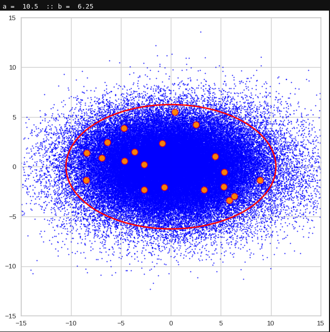
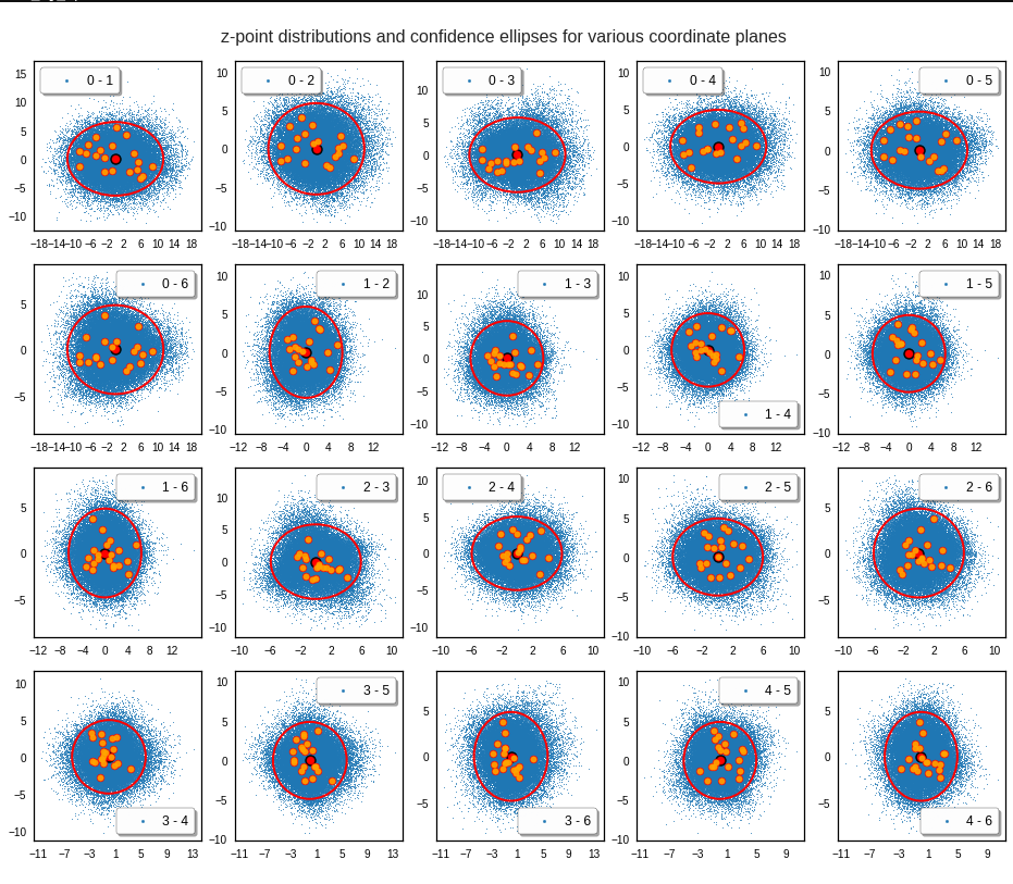
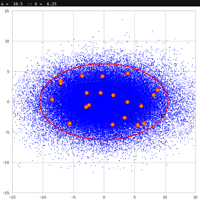
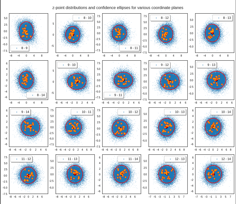
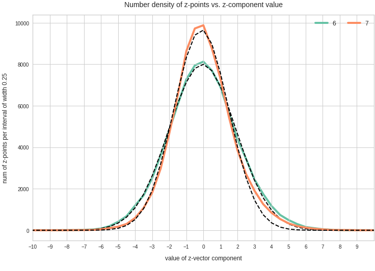
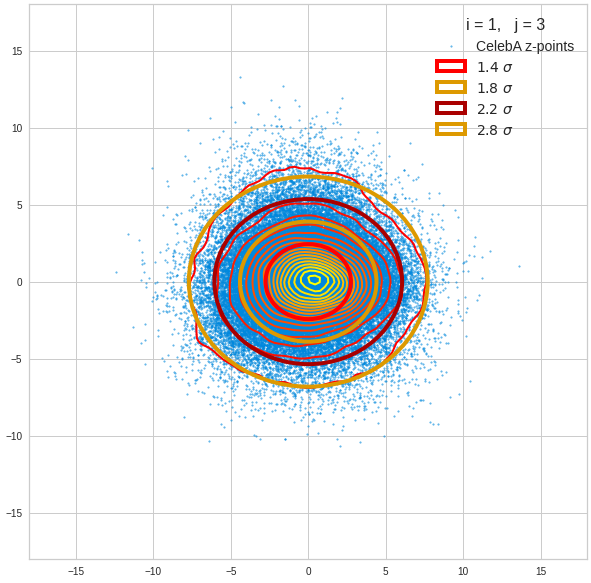
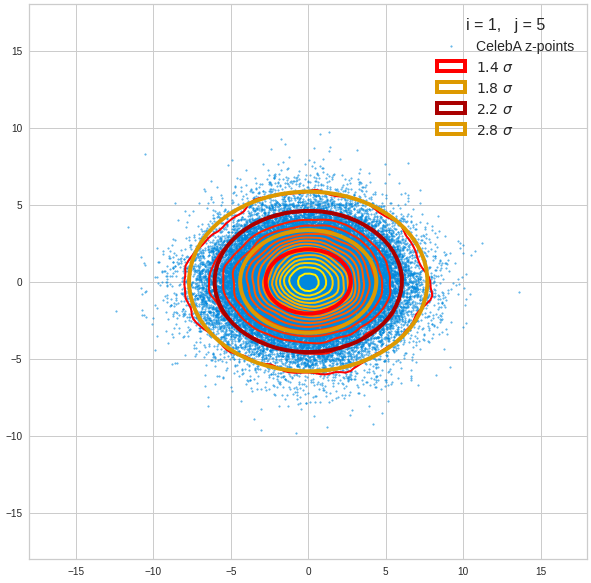
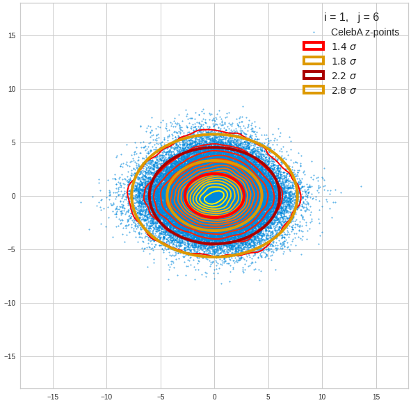
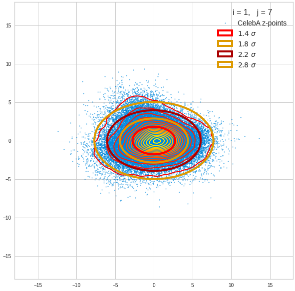
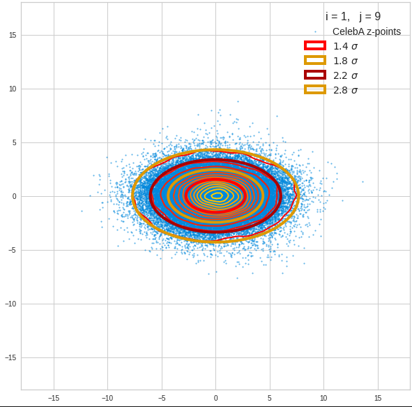
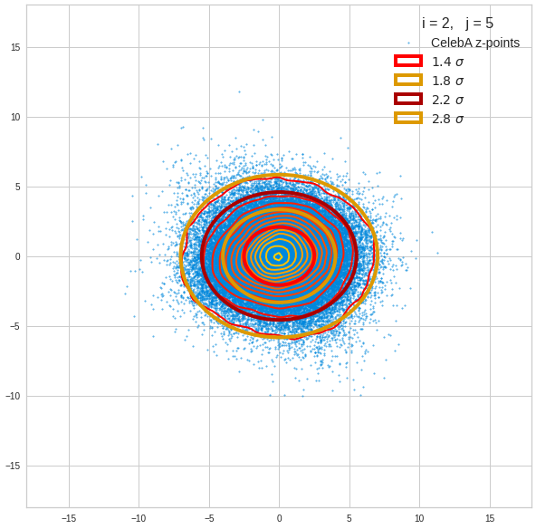
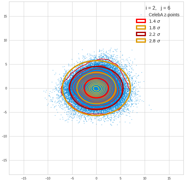
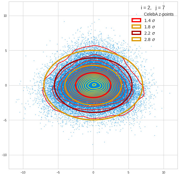
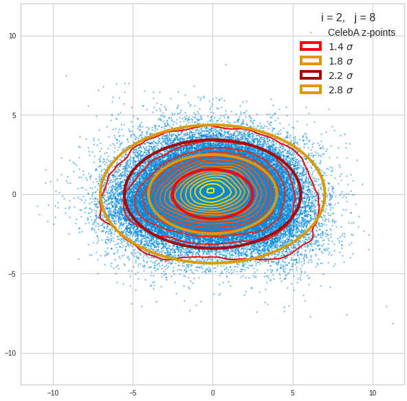
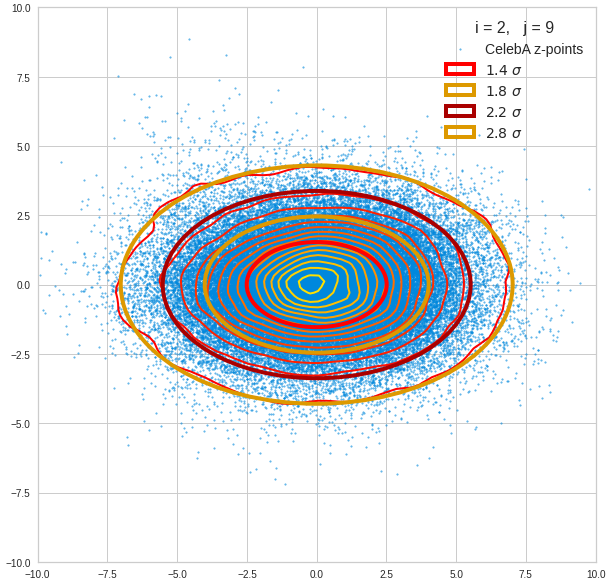
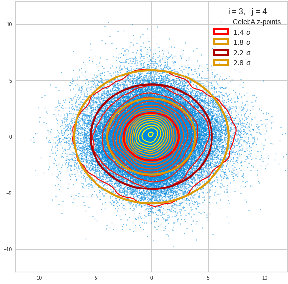
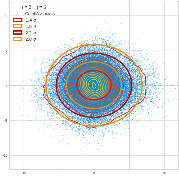
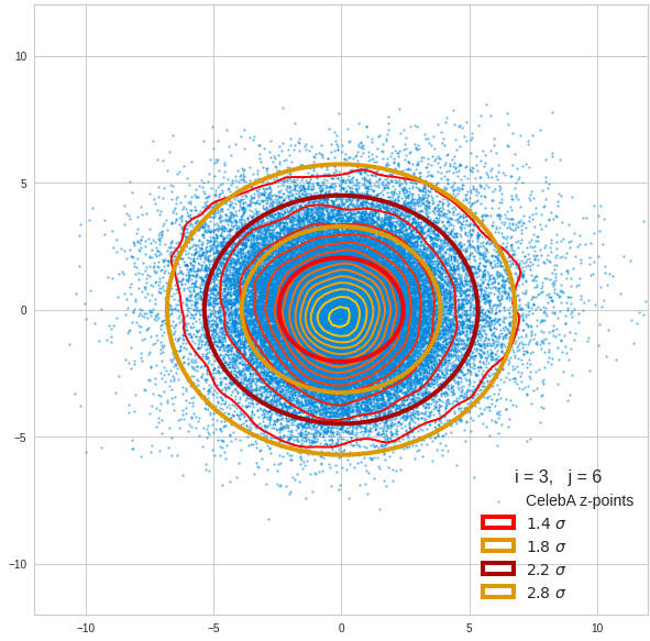
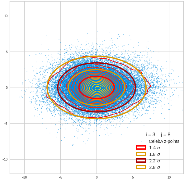
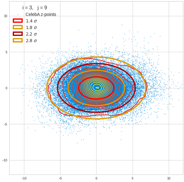
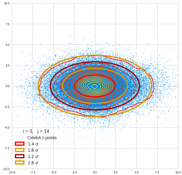
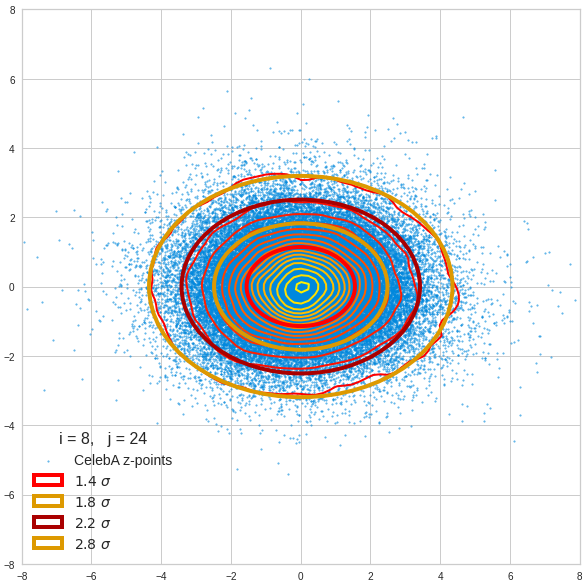
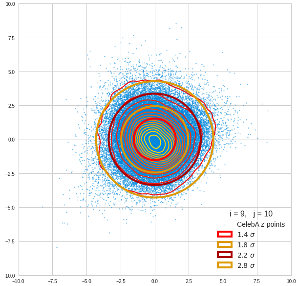
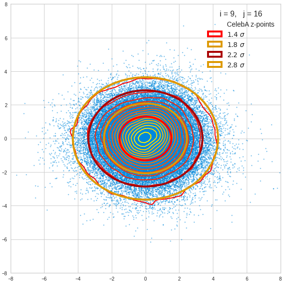
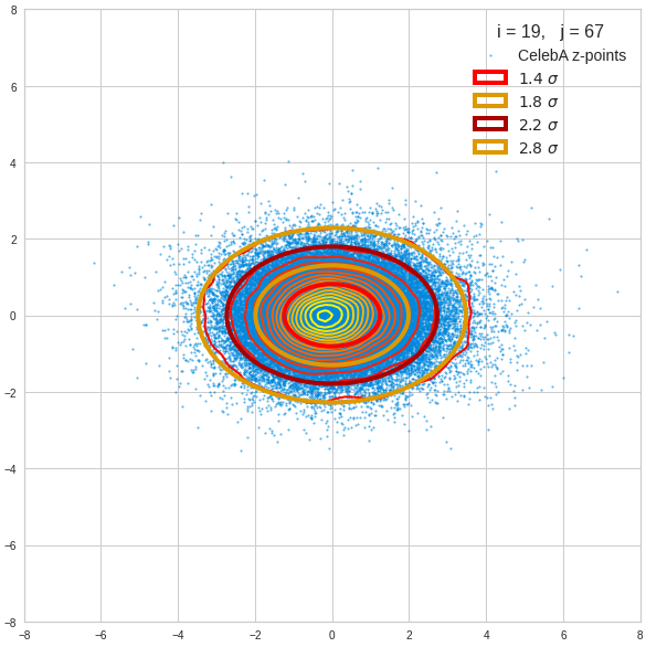
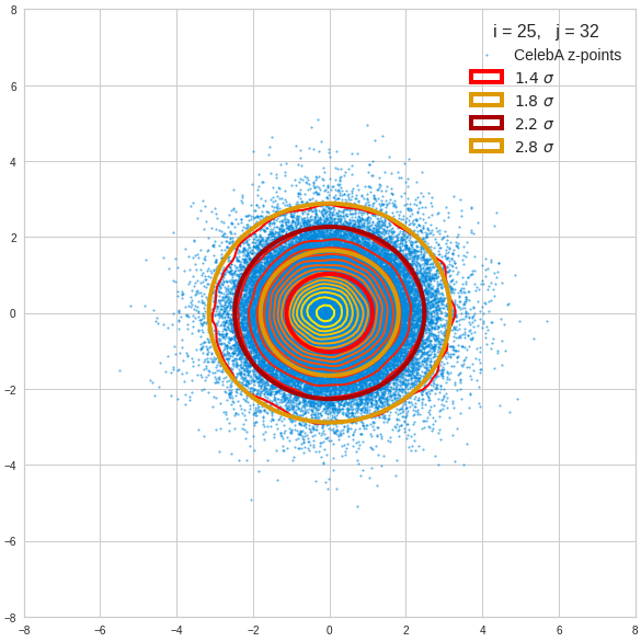
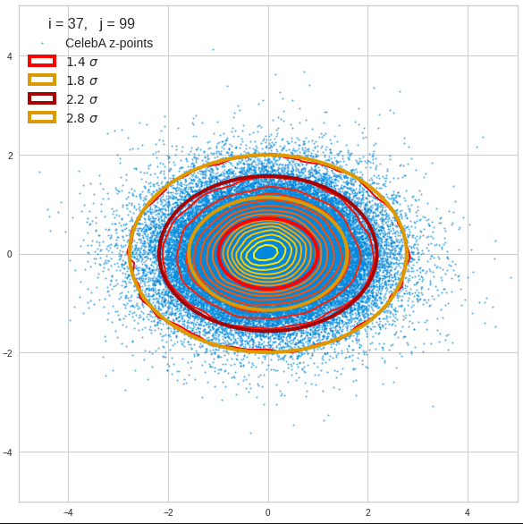
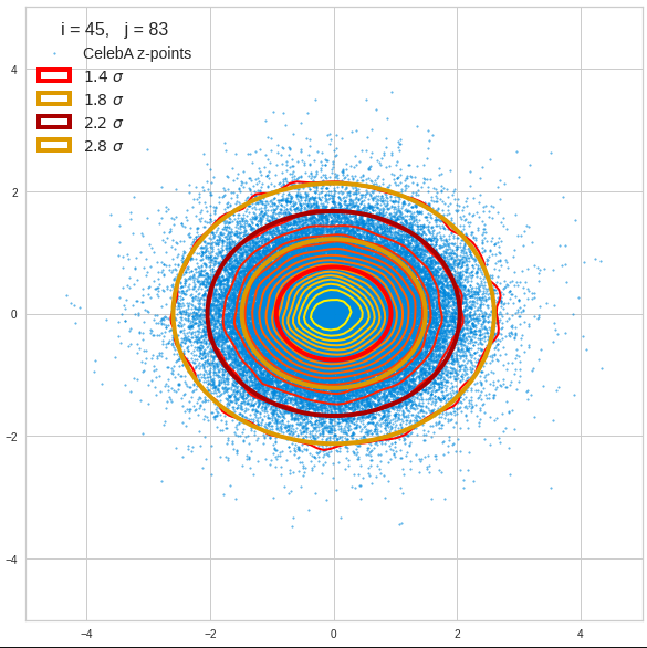
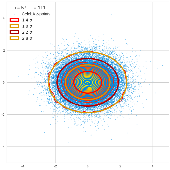
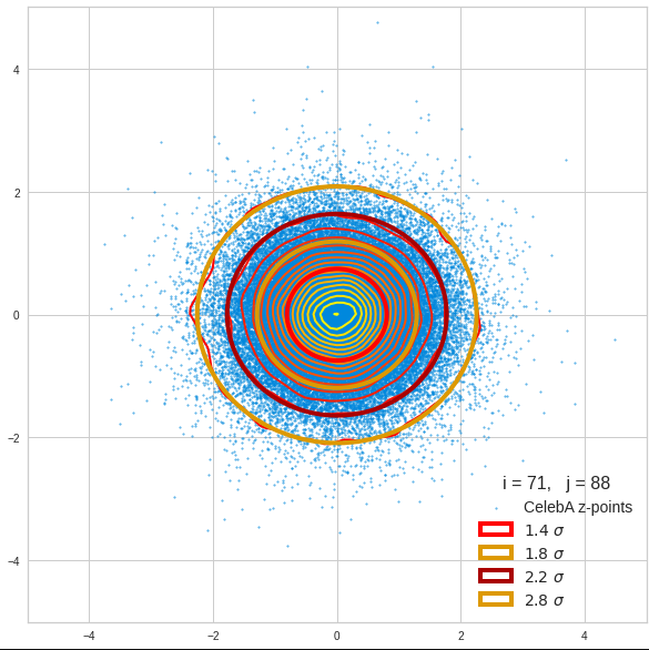
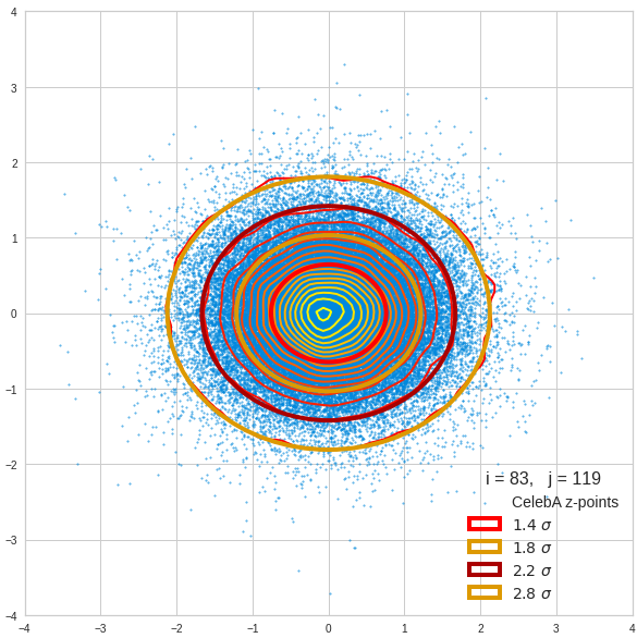
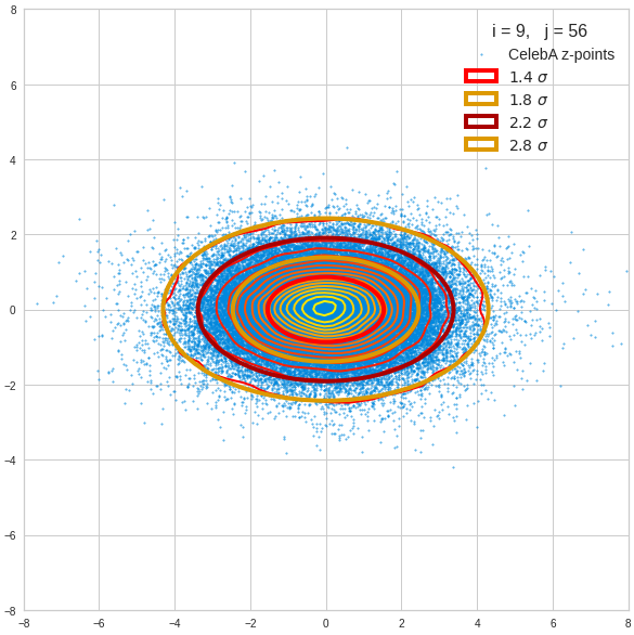
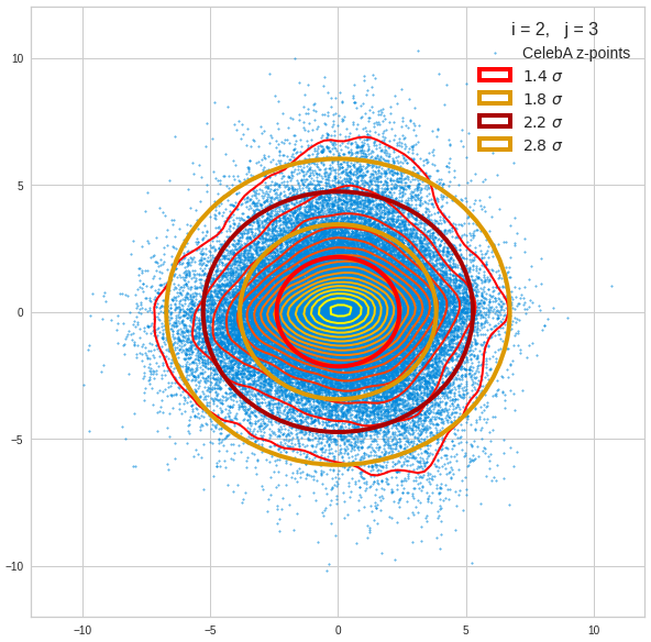
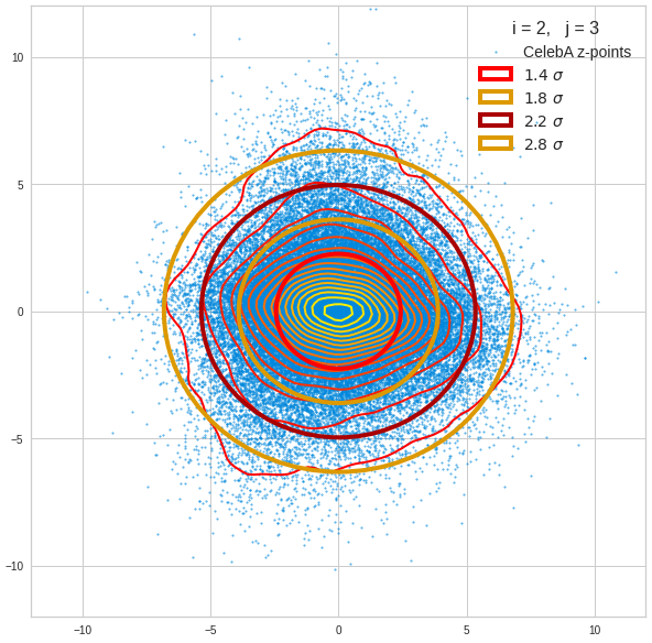
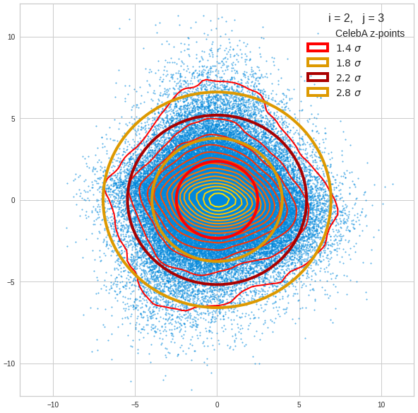
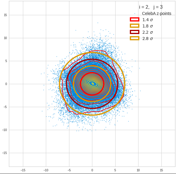
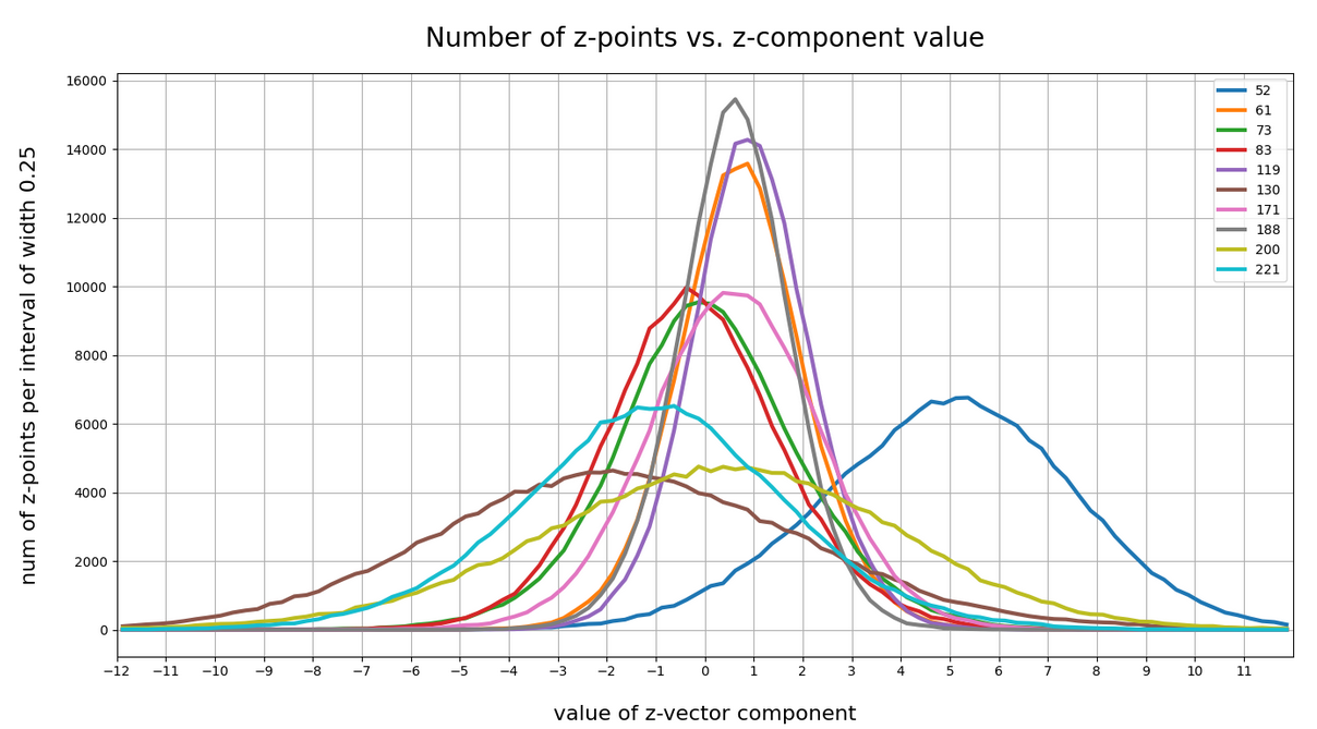
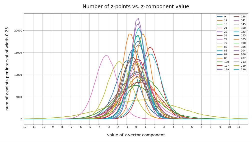
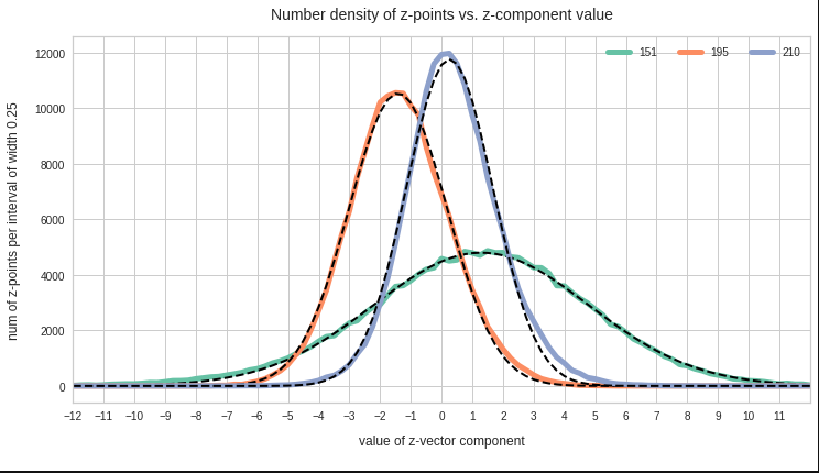
The task of the KL-loss is to compress the data distribution in the latent space and normalize the distribution around certain feature centers there. In the next post
Variational Autoencoder with Tensorflow – IX – taming Celeb A by resizing the images and using a generator
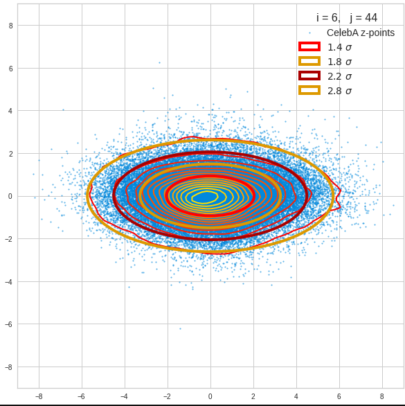
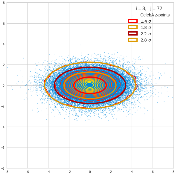
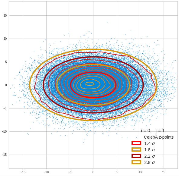
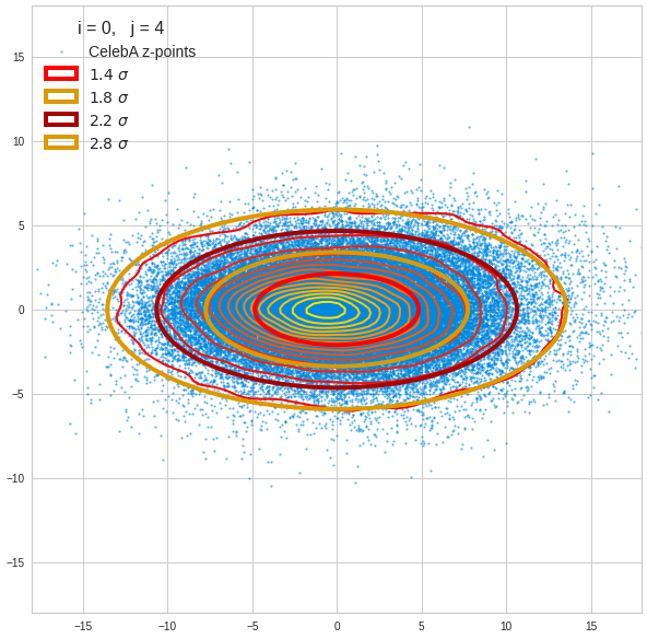
we apply this to images of faces. We shall use the “Celeb A” dataset for this purpose. We are going to see that the scaling factor of the KL loss in this case has to be chosen rather big in comparison to simple cases like MNIST. We will also see that chosing a high dimension of the latent space does not really help to create a reasonable face from statistically chosen points in the latent space.
And before I forget it:
Ceterum Censeo: The worst living fascist and war criminal living today is the Putler. He must be isolated at all levels, be denazified and imprisoned. Long live a free and democratic Ukraine!