
This series of posts is about a special kind of Artificial Neural Networks [ANNs] – namely so called Autoencoders [AEs] and their questionable creative abilities.
The series replaces two previous posts in this blog on a similar topic. My earlier posts were not wrong regarding the results of calculations presented there, but they contained premature conclusions. In this series I hope to perform a somewhat better analysis.
Abilities of Autoencoders and the question of a creative application of AEs
On the one hand side AEs can be trained to encode and compress object information. On the other hand side AEs can decode previously encoded information and reconstruct related original objects from the retrieved information.
A simple application of an AE, therefore, is the compression of image data and the reconstruction of images from compressed data. But, after a suitable adaption of the training process and its input data, we can also use AEs for other purposes. Examples are the denoising of disturbed images or the recoloring of grey images. In the latter cases the reconstructive properties of AEs play an important role.
An interesting question is: Can one utilize the reconstructive abilities of an AE for generative or creative purposes?
This post series will give an answer for the special case of images showing human faces. To say it clearly: I am talking about conventional AEs, not about Variational Autoencoders and neither about state of the art AEs based on transformer technology.
Most text books on Machine Learning [ML] would claim that at least Variational Autoencoders (instead of AEs) are required to create reasonable images of human faces … Well, to trigger a bit of your attention: Below you find some images of human faces created by standard Autoencoder – and NOT by a Variational Autoencoder.
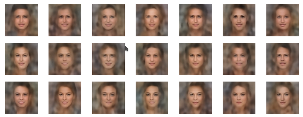
I admit: These pictures are far from perfect, but at least they show clear features of human faces. Not exactly what we expect of a pure conventional Autoencoder fed with statistical input. I apologize for the bias towards female faces, but that is a “prejudice” of the AE caused by my chosen set of training data. And the lack of hairdo-details will later be commented on.
I promise: Analyzing the behavior of conventional AEs is still an interesting topic. Despite many and sophisticated modern alternatives for creative purposes. The reason is that we learn something about the way how an AE organizes the information which it gains during training.
Introductory outline of the problem
A basic expectation considering generative ML-applications would be that the created objects show similar basic features as those presented to the ML-network during training. Also in the case of an AE we want to create new objects of the same class of objects used during training. I.e. objects with the same basic features as those of the training set, but with an individual forming or shape. Generation is not reproduction. We do not want to reproduce any of the digitized objects which were part of the training set. This means that some statistical ingredient in the creation process is required to ensure the production of new objects.
Let us make this clear for the case of images showing human faces. Visualizations of human faces should clearly show all the related characteristic elements like a reasonable oval shape of the face, eyes, eyebrows, nose, lips, ears, human skin color – in a realistic way. Reasonable ranges and limits of color and position values controlling these “features” define our object class.
What we expect of a generative AE application in this case is that we can produce images with human faces having all the named features within allowed limits, but with an individual forming not to be found in the training set. But the faces should look realistic – regarding at least regarding most of the named features. The created objects should fit the class of objects used during training.
Although it is at least in principle possible to create new objects with the help of an AE, one normally runs into trouble regarding this expectation. In the case of images showing a certain kind of objects, an AE most often does not produce pictures with a clear and interpretable content from statistical input fed into the AE’s generative parts. Therefore, most textbooks on Machine Learning recommend to use Variational Autoencoders, GANs or transformers for generative tasks like e.g. the creation of images with “reasonable” contents fitting certain class criteria.
In this series I want to analyze this problem and discuss its cause – for the named special case of images showing human faces. The CelebA dataset will provide us with enough examples to train an AE on the required features. To make the question posed above more concrete for our case:
Can we use an AE trained on CelebA images to construct images showing new human faces with statistical variations in the basic features and their (spatial) correlations?
A key element – the latent space
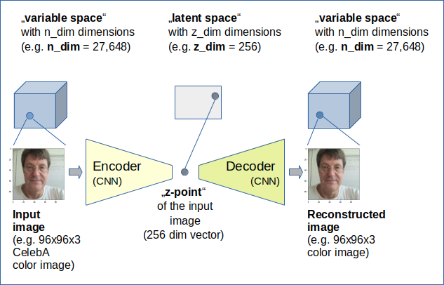
A key element of an AE with respect to generative tasks is the so called “latent space“. This is a multidimensional vector space which the AE uses to encode and compress information about objects seen during training. Every input object presented to the AE is mapped to a point in the latent space. We will call such a point a “z-point” and the latent space also “z-space“. A certain part of an AE can decode object information from a z-point and reconstruct the related original object (with some loss of accuracy in details).
In principle an AE can remap any data point in the latent space to a full-fledged object – in our case an image. We will therefore base the aspired image creation on statistical data points, randomly distributed in the latent space of a trained AE.
During the experiments in the forthcoming posts we will unfortunately find that we fail to construct images with clearly visible faces by applying the AE’s reconstructive part to arbitrarily chosen latent z-points. We will fail even when we restrict the statistically chosen points to a limited spherical or cubic volume around the origin of the latent space.
Data distribution in the latent space
During training an AE creates a specific data point distribution in the latent space. A priori we have no real clue about the shape of this distribution and its impact on creative tasks. But the results of a simple statistical analysis and a PCA-transformation will give us valuable insights regarding the basic shape of the multi-dimensional z-point distribution for CelebA images. We will detect a large coherent fragment with limited extensions, but also filamental structures on small scales. We will conclude that the knowledge an AE acquires during training not only resides in the weights of the neural networks, but also in the spatial structure of the data distribution in the latent space.
The analysis of the large scale fragment will later enable us to actually use an AE for the creation of images with clearly visible faces and respective features. From statistical points, but within certain regions of the latent space. We will also discuss what information the filaments a relatively small scales may encode.
Requirements on the reader’s side
Although I am going to briefly explain some basic elements of AEs in this first post, a reproduction of the calculated results, which I will show in forthcoming posts, requires some practical experience with the architecture and principles of Autoencoders. All data shown in this series have been produced with the help of a convolutional AE, i.e. with an AE based on convolutional layers. The respective neural networks were build with Keras and Tensorflow 2.
Basics representations of images
In this first post I am going to repeat some basics regarding the way AEs work. I will focus on the example of a convolutional AE to extract fundamental features out of images via so called kernel filters. One way to describe the action of an AE is that it basically maps objects of a high-dimensional vector space to objects of a low-dimensional vector space and vice versa. To understand this we have a brief look at the representation of pixel images as vectors or as tensors.
Basics: Representations of images in multidimensional spaces
In Machine Learning objects of interest must be described by characteristic variables. For most objects we need quite many of logically independent variables to cover all of the object properties which are relevant for the objectives of an ML application. The selected set of variables defines a certain class of objects. Each individual object is described by the specific values assigned to its descriptive variables.
Geometrical and vector representation
Independent variables with real values can formally be used to define a basic multidimensional representation space, also called feature space. We span the space geometrically by (orthogonal) coordinate axes – each for a specific one of our descriptive variable. In this geometrical interpretation an individual object is represented by a point in the multidimensional feature space. The point is defined by unique coordinate values – i.e. the individual (real) values the objects has for its variables along the axes. The number of dimensions v_dim of this geometrical space is equal to the number of descriptive variables.
Let us look at the example of images with a certain resolution to get a feeling for the number of dimensions: A quadratic RGB-color image of size 96×96 px has 27648 individual RGB-pixels (96x96x3). In principle we can assign individual values to all of these pixels. (Of course values in certain reasonable range. We also can map the usual integer values in the interval [0,255] to real values in [0.0, 1.0] or [-1.0, 1.0]).
But we can also move on to a more formal and abstract representation of images. The basic reason is that we can calculate with images – at least in principle. We can add and subtract their pixel values or scale them by a factor. Thus we can define images to be elements of a multidimensional vector space. In the above geometrical interpretation a point in the representation space also defines a vector reaching from the origin to the point. This vector has v_dim components which we get by an (orthogonal) projection onto the coordinate axes.
So, an image can be represented by a point in a geometrical coordinate system with 27648 axes or as a vector in a vector space with, of course, the same dimension v_dim = 27648. In our case the vector space has a direct geometrical correlate.
I will call the multidimensional space defined by the independent variables for images below the “image vector space [IVS]]”. We name its number of dimensions “ivs_dim“.
Tensor representation
So far, we have completely abstracted from any meaning which the variables that describe an object may have. Correlations in the abstract geometrical representation or in the vector space can mathematically be detected, but it will be difficult to describe them in a way directly understandable in terms of human object perception. This is motivation enough to order the descriptive data in a different way. Criteria for a new arrangement of the data come from obvious interpretable object properties, but also from efficiency considerations regarding later ML operations.
Let us take an image with 96×96 RGB pixels. The image is characterized by a width, a height and color depth. We have in total 96x96x3 pixels. They can be organized as a long vector with ordered and indexed elements, but we can also arrange them in a 3-dimensional way, namely in form of a 3 dimensional lattice (using width, height, depth as “dimensions”). In NumPy terms we would end up with an array of the shape (96, 96, 3). In terms of Tensorflow this corresponds to a so called tensor of rank 3.
A tensorial representation of an object respects the “meaning” of some variables – often enough a geometrical meaning. In particular, a tensor representation of an image mirrors the 2-dimensional arrangement of pixels and makes it easier to understand pixel correlations in terms of the spatial locations of certain color values on an (x,y)-grid. A human face displayed in an image corresponds to quite many geometrically interpretable correlations of pixel values on such a grid.
Although we technically present input objects to ANNs mostly in form of multi-ranked tensors we can always map such a tensor in a unique way onto a vector (= tensor of rank 1). A mapping of the elements of a tensor of rank 3 on a tensor of rank 1 corresponds to a reshaping of a 3-dimensional NumPy array. A reshaping operation leads to a certain order of the tensor or array components in the resulting vector.
You probably have noticed that we need to be careful to avoid confusion regarding the term “dimension“: On the one hand side it is used to characterize the number of rows, columns, …, i.e. the shape of “multidimensional” arrays (e.g. of Numpy arrays) or tensors. A 2-dimensional array corresponds to a tensor of rank 2. In tensors a specific rank will correspond to a specific number of elements – for our images e.g. 96. Some authors speak of the size of a tensor rank or tensor dimension. However, also a vector space is characterized by a dimension. And there it means the number of linearly independent base vectors that span the vector space.
Whenever I use the term “dimensions” and “dimensionality” in this series I refer to the dimension of the vector space based on the logically independent variables to define our images, i.e. the IVS or the latent space – if not explicitly stated differently. Regarding the dimensions of a tensor I prefer the term rank and when I refer to the sizes of the different sides of a tensor or array I will speak of its shape.
My readers with a background in math or physics should also remember that “tensors” in Machine Learning are very different objects than the (original) tensors used in theoretical physics or mathematics (see my comments on this distinction at here).
The layers of modern ANNs perform complex operations on their tensorially ordered input data. They can change the shape of tensors and even their rank.
Basic elements and features of Autoencoders
An Autoencoder solves two tasks – each of which is covered by a special neural network:
- An Encoder network encodes information about objects which can be described as vectors of an IVS.
- A Decoder network decodes previously encoded information and reconstructs related objects in the IVS.
Both networks can be coupled to each other by feeding the output of the Encoder as input into the Decoder. This is done during the training of an AE. The Encoder and the Decoder networks constitute the full AE. But both sub-networks can also be used individually.
Latent space – and inversion of Encoder operation by the Decoder
The Encoder network mathematically maps objects of the IVS, which are presented to the ANN in tensorial form, onto vectors in another vector space which typically has a much lower number of dimensions. This target space of the Encoder is called the “latent space“.
In this post series we will sometimes also use “z-space” as a synonym. Let us name number of dimensions of the latent space z_dim.
The latent space can be represented by a z_dim-dimensional coordinate system (with orthogonal axes). Let us call a point in the latent space a “z-point“. Each z-point corresponds to a “latent vector” pointing from the origin of the coordinate system to this z-point. Projections of the vector onto the coordinate axes give us its z_dim components. Note that the components take real values. At least in principle we are able to perform vector arithmetics in the latent space. Whatever the results may mean …
In many AE-applications the latent space has much fewer dimensions than the IVS:
ivs_dim >> z_dim
I.e. the Encoder typically compresses information whilst it maps input objects onto vectors and related z-points) in the latent space.
The Decoder instead maps points in the latent space back onto points in the IVS. I.e. the Decoder inverses the mapping function of the Encoder – in a way. We expect that the Decoder’s functionality comes very close to the inverse of the Encoder’s functionality. I.e., when we
- first execute an encoding process for an image “Img_IMX” with the help of the Decoder, which produces a z_point “z_imx” for Img_IMX
- and then execute a decoding process for z_imx which results in an image Img_OMX
we expect that the Decoder shall reproduce IMX as closely as possible. Ideally we would like to see
Img_OMX = Img_IMX
But AEs are of course not that good – even if z_dim is big. And we all know that we should be careful with the precision of ANNs, as we need a solid balance of detail reproduction and generalization for all ML-algorithms. For an AE a relation Img_OMX = Img_IMX would mean overfitting.
The latent space obviously is an intermediate space connecting Encoder and Decoder. To give meaningful results both the Encoder and the Decoder of an AE model have to be trained simultaneously to fulfill Img_OMX = Img_IMX as good as possible.
Note that the Decoder of a trained AE can and will create a complex object in the IVS for any data point in the latent space. A Decoder basically is nothing else than a mathematical mapping machine which can work with any input, as long as it fulfills required formal conditions.
Orthogonal coordinate systems
Both the IVS and the latent space will in our examples be described by orthogonal coordinate systems. This allows for a simple definition of vector lengths by using a L2-norm. This will help us to analyze e.g. the z-point-distribution vs. a multidimensional “radius”, measured from the origin of the latent space.
In the course of our coming numerical experiments we do not care about transformations to non-orthogonal systems. However, we will later apply the method of a PCA-analysis to data point distributions in the latent space. This will correspond to transformations to coordinate systems with a shifted origin and rotated coordinate axes in comparison to the original coordinate system of the latent space. But these linear PCA transformations keep up the orthogonality of the coordinate axes.
Overview: Encoder, latent space, Decoder
The following sketch gives an overview over the working of an AE, which we want to train to simply encode images and decode images.
As both the Encoder and Decoder will be represented by Deep Neural Networks the mapping functions are non-linear in both cases. This is due to the activation functions of the neurons. As some typically used activation functions (as e.g. ReLU) exhibit points where the first derivative becomes dis-continuous, not all z-points created during training may form a continuously coherent manifold.
Furthermore, it is important to note that not all vectors in the input image space do represent meaningful image content. Equivalently, not all z-points in the latent space will lead to meaningful images in the input variable space after an application of the Decoder either.
Statistical z-points for generative tasks
We will train a concrete AE with CelebA images. A trained Decoder should be able to do something with any z-point fed into it.
However, whether the reconstructed output – an image – shows something reasonable is another question. We will base our investigation on points statistically distributed over a limited (multi-dimensional) area around the origin of the latent space. Our naive hope is that we by chance hit regions that lead to the creation of images with clear human faces. We will find, however, that this may not often be the case for certain generators of statistical vectors.
Layer structure of a suitable convolutional AE and self-supervised training
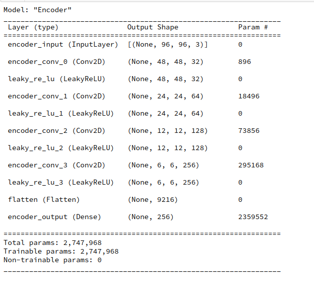
How do we technically realize the Encoder and Decoder networks? I have made my life simple by just using convolutional and transposed convolutional layers provided by the Keras framework. The Encoder got 4 convolutional Conv2D layers. The Decoder instead comprised a series of 4 corresponding Conv2DTranspose layers.
Convolutional layers in the Encoder are well suited for the extraction of basic patterns in input images. In the Decoder transposed convolutional layers can handle the task to combine elementary patterns on different length-scales to reconstruct an image displaying the encoded information.
The layer structure was also established with the help of Keras’ functional model. Below you find details of the layer structures. The full AE model was afterwards constructed by combining both the Encoder and Decoder network models into a common AE model (again with the help of Keras).
Encoder
Decoder
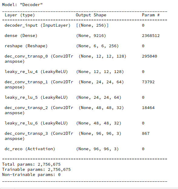
The reader notices that our AE was prepared to work with images of the size 96×96 px.
Actually, the reproduction quality was a bit better for other layer sequences [ Encoder: (64, 64, 128, 128) / Decoder: (128, 128, 64, 64)], other activation functions and a MSE- instead of a BCE-cost-function. But this is not so important in our context.
We trained the resulting AE by feeding input images to the Encoder. This resulted in z-points which were directly fed into the Decoder. The difference of the Decoder’s output image to the original input image was then used as the argument of a cost function to be optimized during training. I used a Binary Cross-Entropy [BCE] cost function.
As we use the input image itself as a target label the training runs for our AE are self-supervised runs.
CelebA
The Celeb A data set contains images of around 200,000 faces with varying contours, hairdos and very different, inhomogeneous backgrounds. And the faces are displayed from different viewing angles.
My AE was trained on 170,000 statistically selected CelebA images for 24 epochs with a very small original step size (5.e-4) and an Adam optimizer. The original CelebA images were reduced to a size of 96×96 pixels.
The simple case of encoding and decoding CelebA images – and a minimum of latent space dimensions
Let us say that we have quadratic images with dimensions 96×96 px. Then the IVS dimension is
ivs_dim = (96 x 96 x 3) = 27,648.
A compression of data requires the usage of correlations. Images of a face show many such correlations: There is a certain symmetry in a face, the nose is horizontally placed somewhere near the middle of the eyes and vertically somewhere between the eyes and the mouth. Still, the minimum number of dimensions required to encode the information about details of a face reasonably is much larger than 2, 3 or even 10. Think of the number of elements in a Fourier series required to approximate details of an image. This number can go up to hundreds if small details have to be covered well.
Experience shows that we need a latent space dimension
256 ≤ z_dim ≤ 2000
to reproduce details of face-images reasonably well also for images not following the style and conventions of CelebA. Below you see the original of my face and the reproduction of an AE with z_dim = 1600 after 18 epochs:

However, throughout this post series we will use a value of only
z_dim = 256
This helps us to keep the numerical efforts within affordable limits. So our Encoder will map vectors with more than 27,000 components to vectors with only 256 components. Details of nose, eyebrows, lips and hair will get lost – and the remaining resemblance is only an overall stereotype one. To give you an example I show you a section of a typical reconstruction which is relatively far away from the original.
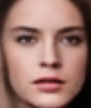
Very idealized, symmetrized and smoothed out – at least in comparison to the original (which I can not show due to legal rights considerations).
Though much smaller than 27648, a latent space with z_dim=256 has a relatively high dimensionality. A data distribution in such a space is a bit more difficult to analyze than in two or three dimensions.
Conclusion
An AE can encode and at the same time compress information about faces shown on images. For the images of the CelebA dataset we need to choose a minimum dimension of the latent space of about 200 to cover the most important correlations between pixels showing a face. Still a lot of detail information is lost.
After training of both the Encoder and Decoder of an AE the Decoder should be able to create images out of any point in the latent space. The question is whether we get reasonable face images for image reconstructions based on randomly chosen z-points in the latent space.
In the next post(s)
Autoencoders and latent space fragmentation – II – number distributions for vector component values
of this series we will look at information about the z-point distribution created for CelebA images. We will then compare characteristic properties of this distribution to those of a vector distribution created by a specific statistical generator.