In a previous article series
A simple Python program for an ANN to cover the MNIST dataset – I – a starting point
we have played with a Python/Numpy code, which created a configurable and trainable “Multilayer Perceptron” [MLP] for us. See also
MLP, Numpy, TF2 – performance issues – Step I – float32, reduction of back propagation
for ongoing code and performance optimization.
A MLP program is useful to study multiple topics in Machine Learning [ML] on a basic level. However, MLPs with dense layers are certainly not at the forefront of ML technology – though they still are fundamental bricks in other more complicated architectures of “Artifical Neural Networks” [ANNs]. During my MLP experiments I became sufficiently acquainted with Python, Jupyter and matplotlib to make some curious first steps into another field of Machine Learning [ML] now: “Convolutional Neural Networks” [CNNs].
CNNs on my level as an interested IT-affine person are most of all fun. Nevertheless, I quickly found out that a somewhat systematic approach is helpful – especially if you later on want to use the Tensorflow’s API and not only Keras. When I now write about some experiments I did and do I summarize my own biased insights and sometimes surprises. Probably there are other hobbyists as me out there who also fight with elementary points in the literature and practical experiments. Books alone are not enough … I hope to deliver some practical hints for this audience. The present articles are, however, NOT intended for ML and CNN experts. Experts will almost certainly not find anything new here.
Although I address CNN-beginners I assume that people who stumble across this article and want to follow me through some experiments have read something about CNNs already. You should know fundamentals about filters, strides and the basic principles of convolution. I shall comment on all these points but I shall not repeat the very basics. I recommend to read relevant chapters in one of the books I recommend at the end of this article. You should in addition have some knowledge regarding the basic structure and functionality of a MLP as well as “gradient descent” as an optimization technique.
The objective of this introductory mini-series is to build a first simple CNN, to apply it to the MNIST dataset and to visualize some of the elementary “features” a CNN allegedly detects in the images of handwritten digits – at least according to many authors in the field of AI. We shall use Keras (with the Tensorflow 2.2 backend and CUDA 10.2) for this purpose. And, of course, a bit of matplotlib and Python/Numpy, too. We are working with MNIST images in the first place – although CNNs can be used to analyze other types of input data. After we have covered the simple standard MNIST image set, we shall also work a bit with the so called “MNIST fashion” set.
But in this article I start with some introductory words on the structure of CNNs and the task of its layers. We shall use the information later on as a reference. In the second article we shall set up and test a simple version of a CNN. Further articles will then concentrate on visualizing what a trained CNN reacts to and how it modifies and analyzes the input data on its layers.
Why CNNs?
When we studied an MLP in combination with the basic MNIST dataset of handwritten digits we found that we got an improvement in accuracy (for the same setup of dense layers) when we pre-processed the data to find “clusters” in the image data before training. Such a process corresponds to detecting parts of an MNIST image with certain gray-white pixel constellations. We used Scikit-Learn’s “MiniBatchKMeans” for this purpose.
We saw that the identification of 40 to 70 cluster areas in the images helped the MLP algorithm to analyze the MNIST data faster and better than before. Obviously, training the MLP with respect to combinations of characteristic sub-structures of the different images helped us to classify them as representations of digits. This leads directly to the following question:
What if we could combine the detection of sub-structures in an image with the training process of an ANN?
CNNs seem to the answer! According to teaching books they have the following abilities: They are designed to detect elementary structures or patterns in image data (and other data) systematically. In addition they are enabled to learn something about characteristic compositions of such elementary features during training. I.e., they detect more abstract and composite features specific for the appearance of certain objects within an image. We speak of a “feature hierarchy“, which a CNN can somehow grasp and use – e.g. for classification tasks.
While a MLP must learn about pixel constellations and their relations on the whole image area, CNNs are much more flexible and even reusable. They identify and remember elementary sub-structures independent of the exact position of such features within an image. They furthermore learn “abstract concepts” about depicted objects via identifying characteristic and complex composite features on a higher level.
This simplified description of the astonishing capabilities of a CNN indicates that its training and learning is basically a two-fold process:
- Detecting elementary structures in an image (or other structured data sets) by filtering and extracting patterns within relatively small image areas. We shall call these areas “filter areas”.
- Constructing abstract characteristic features out of the elementary filtered structural elements. This corresponds to building a “hierarchy” of significant features for the classification of images or of distinguished objects or of the positions of such objects within an image.
Now, if you think about the MNIST digit data we understand intuitively that written digits represent some abstract concepts like certain combinations of straight vertical and horizontal line elements, bows and line crossings. The recognition of certain feature combinations of such elementary structures would of course be helpful to recognize and classify written digits better – especially when the recognition of the combination of such features is independent of their exact position on an image.
So, CNNs seem to open up a world of wonders! Some authors of books on CNNs, GANs etc. praise the ability to react to “features” by describing them as humanly interpretable entities as e.g. “eyes”, “feathers”, “lips”, “line segments”, etc. – i.e. in the sense of entity conceptions. Well, we shall critically review this idea, which I think is a misleading over-interpretation of the capacities of CNNs.
Filters, kernels and feature maps
An important concept behind CNNs is the systematic application of (various) filters (described and defined by so called “kernels”).
A “filter” defines a kind of masking pixel area of limited small size (e.g. 3×3 pixels). A filter combines weighted output values at neighboring nodes of a input layer in a specific defined way. It processes the offered information in a defined area always in the same fixed way –
independent of where the filter area is exactly placed on the (bigger) image (or a processed version of it). We call a processed version of an image a “map“.
A specific type of CNN layer, called a “Convolution Layer” [Conv layer], and a related operational algorithm let a series of such small masking areas cover the complete surface of an image (or a map). The first Conv layer of a CNN filters the information of the original image information via a multitude of such masking areas. The masks can be arranged overlapping, i.e. they can be shifted against each other by some distance along their axes. Think of the masking filter areas as a bunch of overlapping tiles covering the image. The shift is called stride.
The “filter” mechanism (better: the mathematical recipe) of a specific filter remains the same for all of its small masking areas covering the image. A specific filter emphasizes certain parts of the original information and suppresses other parts in a defined way. If you combine the information of all masks you get a new (filtered) representation of the image – we speak of a “feature map” – sometimes with a smaller size than the original image (or map) the filter is applied to. The blending of the original data with a filtering mask creates a “feature map“, i.e. a filtered view onto the input data. The blending process is called “convolution” (due to the related mathematical operations).
The picture below sketches the basic principle of a 3×3-filter which is applied with a constant stride of 2 along each axis of the image:
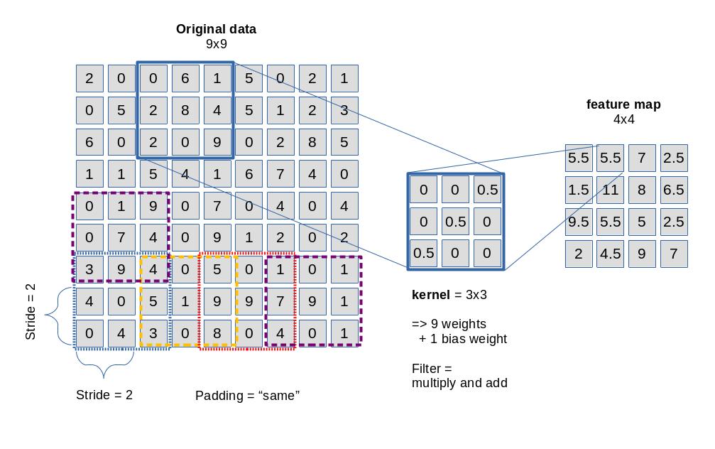
Convolution is not so complicated as it sounds. It means: You multiply the original data values in the covered small area by factors defined in the filter’s kernel and add the resulting values up to get a a distinct value at a defined position inside the map. In the given example with a stride of 2 we get a resulting feature map of 4×4 out of a original 9×9 (image or map).
Note that a filter need not be defined as a square. It can have a rectangular (n x m) shape with (n, m) being integers. (In principle we could also think of other tile forms as e.g. hexagons – as long as they can seamlessly cover a defined plane. Interesting, although I have not seen a hexagon based CNN in the literature, yet).
A filter’s kernel defines factors used in the convolution operation – one for each of the (n x m) defined points in the filter area.
Note also that filters may have a “depth” property when they shall be applied to three-dimensional data sets; we may need a depth when we cover colored images (which require 3 input layers). But let us keep to flat filters in this introductory discussion …
Now we come to a central question: Does a CNN Conv layer use just one filter? The answer is: No!
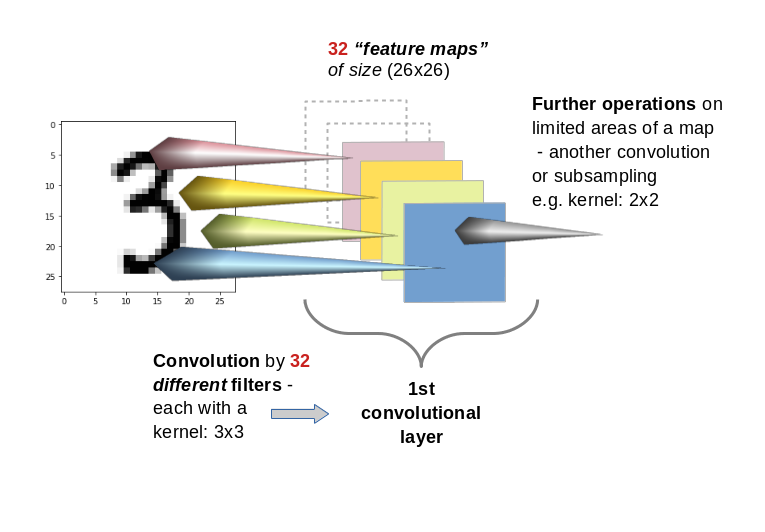
A Conv layer of a CNN you allows for the construction of multiple different filters. Thus we have to deal with a whole bunch of filters per each convolutional layer. E.g. 32 filters for the first convolutional layer and 64 for the second and 128 for the third. The outcome of the respective filter operations is the creation is of equally many “feature maps” (one for each filter) per convolutional layer. With 32 different filters on a Conv layer we would thus build 32 maps at this layer.
This means: A Conv layer has a multitude of sub-layers, i.e. “maps” which result of the application of different filters on previous image or map data.
You may have guessed already that the next step of abstraction is:
You can apply filters also to “maps” of previous filters, i.e. you can chain convolutions. Thus, feature maps are either connected to the image (1st Conv layer) or to the maps of a previous layer.
By using a sequence of multiple Conv layers you cover growing areas of the original image. Everything clear? Probably not …
Filters and their related weights are the end products of the training and optimization of a CNN!
When I first was confronted with the concept of filters, I got confused because many authors only describe the basic technical details of the “convolution” mechanism. They explain with many words how a filter and its kernel work when the filtering area is “moved” across the surface of an image. They give you pretty concrete filter examples; very popular are straight lines and crosses indicated by “ones” as factors in the filter’s kernel and zeros otherwise. And then you get an additional lecture on strides and padding. You have certainly read various related passages in books about ML and/or CNNs. A pretty good example for this “explanation” is the (otherwise interesting and helpful!) book of Deru and Ndiaye (see the bottom of this article. I refer to the introductory chapter 3.5.1 on CNN architectures.)
Well, the technical procedure is pretty easy to understand from drawings as given above – the real question that nags in your brain is:
“Where the hell do all the different filter definitions come from?”
What many authors forget is a central introductory sentence for beginners:
A filter is not given a priori. Filters (and their kernels) are systematically constructed and build up during the training of a CNN; filters are the end products of a learning and optimization process every CNN must absolve.
This means: For a given problem or dataset you do not know in advance what the “filters” (and their defining kernels) will look like after training (aside of their pixel dimensions already fixed by the CNN’s layer definitions). The “factors” of a filter used in the convolution operation are actually weights, whose final values are the outcome of a learning process. Just as in MLPs …
Nothing is really “moved” …
Another critical point is the somewhat misleading analogy of “moving” a filter across an image’s or map’s pixel surface. Nothing is ever actually “moved” in a CNN’s algorithm. All masks are already in place when the convolution operations are performed:
Every element of a specific e.g. 3×3 kernel corresponds to “factors” for the convolution operation. What are these factors? Again: They are nothing else but weights – in exactly the same sense as we used them in MLPs. A filter kernel represents a set of weight-values to be multiplied with original output values at the “nodes” in other layers or maps feeding input to the nodes of the present map.
Things become much clearer if you imagine a feature map as a bunch of arranged “nodes”. Each node of a map is connected to (n x m) nodes of a previous set of nodes on a map or layer delivering input to the Conv layer’s maps.
Let us look at an example. The following drawing shows the connections from “nodes” of a feature map “m” of a Conv layer L_(N+1) to nodes of two different maps “1” and “2” of
Conv layer L_N. The stride for the kernels is assumed to be just 1.
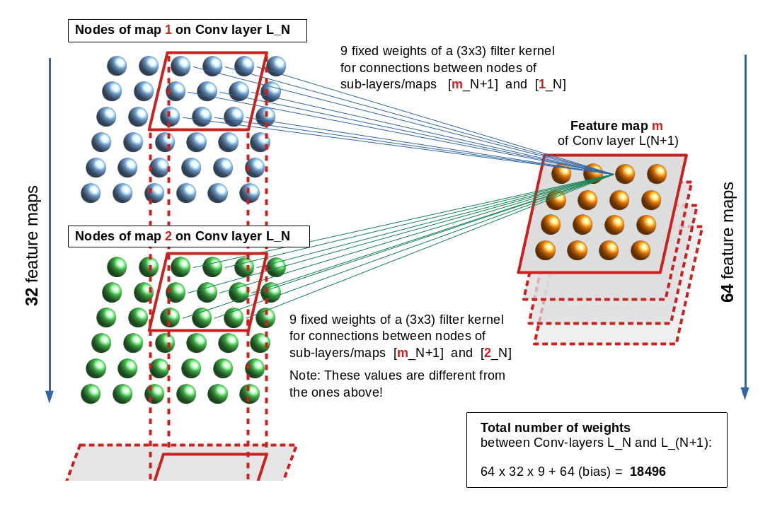
In the example the related weights are described by two different (3×3) kernels. Note, however, that each node of a specific map uses the same weights for connections to another specific map or sub-layer of the previous (input) layer. This explains the total number of weights between two sequential Conv layers – one with 32 maps and the next with 64 maps – as (64 x 32 x 9) + 64 = 18496. The 64 extra weights account for bias values per map on layer L_(N+1). (As all nodes of a map use fixed bunches of weights, we only need exactly one bias value per map).
Note also that a stride is defined for the whole layer and not per map. Thus we enforce the same size of all maps in a layer. The convolutions between a distinct map and all maps of the previous layer L_N can be thought as operations performed on a column of stacked filter areas at the same position – one above the other across all maps of L_N. See the illustration below:
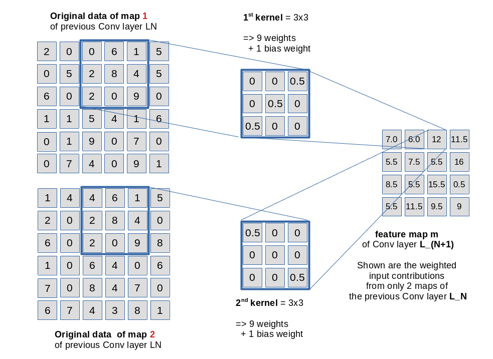
The weights of a specific kernel work together as an ensemble: They condense the original 3×3 pixel information in the filtered area of the connected input layer or a map to a value at one node of the filter specific feature map. Please note that there is a bias weight in addition for every map; however, at all masking areas of a specific filter the very same 9 weights are applied. See the next drawing for an illustration of the weight application in our example for fictitious node and kernel values.
A CNN learns the appropriate weights (= the filter definitions) for a given bunch of images via training and is guided by the optimization of a loss function. You know these concepts already from MLPs …
The difference is that the ANN now learns about appropriate “weight ensembles” – eventually (!) working together as a defined convolutional filter between different maps of neighboring Conv (and/or sampling ) Layers. (For sampling see a separate paragraph below.)
The next picture illustrates the column like convolution of information across the identically positioned filter areas across multiple maps of a previous convolution layer:
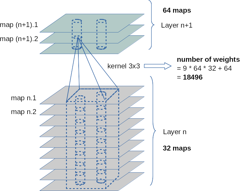
The fact that the weight ensemble of a specific filter between maps is always the same, explains, by the way, the relatively (!) small number of weight parameters in deep CNNS.
Intermediate summary: The weights, which represent the factors used by a specific filter operation called convolution, are defined during a training process. The filter, its kernel and the respective weight values are the outcome of a mathematical optimization process – mostly guided by gradient descent.
Activation functions
As in MLPs each Conv layer has an associated “activation function” which is applied at each node of all maps after the resulting values of the convolution have been calculated as
the nodes input. The output then feeds the connections to the next layer. In CNNs for image handling often “Relu” or “Selu” are used as activation functions – and not “sigmoid” which we applied in the MLP code discussed in another article series of this blog.
Tensors
The above drawings indicate already that we need to arrange the data (of an image) and also the resulting map data in an organized way to be able to apply the required convolutional multiplications and summations the right way.
An colored image is basically a regular 3 dimensional structure with a width “w” (number of pixels along the x-axis), a height “h” (number of pixels along the y-axis) and a (color) depth “d” (d=3 for RGB colors).
If you represent the color value at each pixel and RGB-layer by a float you get a bunch of w x h x d float values which we can organize and index in a 3 dimensional Numpy array. Mathematically such well organized arrays with a defined number of axes (rank), a set of numbers describing the dimension along each axis (shape), a data-type, possible operations (and invariance aspects) define an abstract object called a “tensor“. Colored image data can be arranged in 3-dimensional tensors; gray colored images in a pseudo 3D-tensor which has a shape of (n, m, 1). (Keras and Tensorflow want to get imagedata in form of 2D tensors).
Now the important point is: The output data of Conv-layers and their feature maps also represent tensors. A bunch of 32 maps with a defined width and height defines data of a 3D-tensor.
You can imagine each value of such a tensor as the input or output given at a specific node in a layer with a 3-dimensional sub-structure. (In other even more complex data structures than images we would other multi-dimensional data structures.) The weights of a filter kernel describe the connections of the nodes of a feature map on a layer L_N to a specific map of a previous layer. Weights, actually, also define elements of a tensor.
The forward- and backward-propagation operations performed throughout such a complex net during training thus correspond to sequences of tensor-operations – i.e. generalized versions of the np.dot()-product we got to know in MLPs.
You understood already that e.g strides are important. But you do not need to care about details – Keras and Tensorflow will do the job for you! If you want to read a bit look a the documentation of the TF function “tf.nn.conv2d()”.
When we later on train with mini-batches of input data (i.e. batches of images) we get yet another dimension of our tensors. This batch dimension can – quite similar to MLPs – be used to optimize the tensor operations in a vectorized way. See my series on MLPs.
Chained convolutions cover growing areas of the original image
Two sections above I characterized the training of a CNN as a two-fold procedure. From the first drawing it is relatively easy to understand how we get to grasp tiny sub-structures of an image: Just use filters with small kernel sizes!
Fine, but there is probably a second question already arising in your mind:
By what mechanism does a CNN find or recognize a hierarchy of features?
One part of the answer is: Chain convolutions!
Let us assume a first convolutional layer with filters having a stride of 1 and a (3×3) kernel. We get maps with a shape of (26, 26) on this layer. The next Conv layer shall use a (4×4) kernel and also a stride of 1; then we get maps with a shape of (23, 23). A node on the second layer covers (6×6)-arrays on the original image. Two neighboring nodes a total area of (7×7). The individual (6×6)-areas of course overlap.
With a stride of 2 on each Conv-layer the corresponding areas on the original image are (7×7) and (11×11).
So a stack of consecutive (sequential) Conv-layers covers growing areas on the original image. This supports the detection of a pattern or feature hierarchy in the data of the input images.
However: Small strides require a relatively big number of sequential Conv-layers (for 3×3 kernels and stride 2) at least 13 layers to eventually cover the full image area.
Even if we would not enlarge the number of maps beyond 128 with growing layer number, we would get
(32 x 9 + 32) + (64 x 32 +64) + (128 x 64 + 128) + 10 x (128 x 128 + 128) = 320 + 18496 + 73856 + 10*147584 = 1.568 million weight parameters
to take care of!
This number has to be multiplied by the number of images in a mini-batch – e.g. 500. And – as we know from MLPs we have to keep all intermediate output results in RAM to accelerate the BW propagation for the determination of gradients. Too many data and parameters for the analysis of small 28×28 images!
Big strides, however, would affect the spatial resolution of the first layers in a CNN. What is the way out?
Sub-sampling is necessary!
The famous VGG16 CNN uses pairs and triples of convolution chains in its architecture. How does such a network get control over the number of weight parameters and the RAM requirement for all the output data at all the layers?
To get information in the sense of a feature hierarchy the CNN clearly should not look at details and related small sub-fields of the image, only. It must cover step-wise growing (!) areas of the original image, too. How do we combine these seemingly contradictory objectives in one training algorithm which does not lead to an exploding number of parameters, RAM and CPU time? Well, guys, this is the point where we should pay due respect to all the creative inventors of CNNs:
The answer is: We must accumulate or sample information across larger image or map areas. This is the (underestimated?) task of pooling– or sampling-layers.
For me it was just another confusing point in the beginning – until one grasps the real magic behind it. At first sight a layer like a typical “maxpooling” layer seems to reduce information, only; see the next picture:
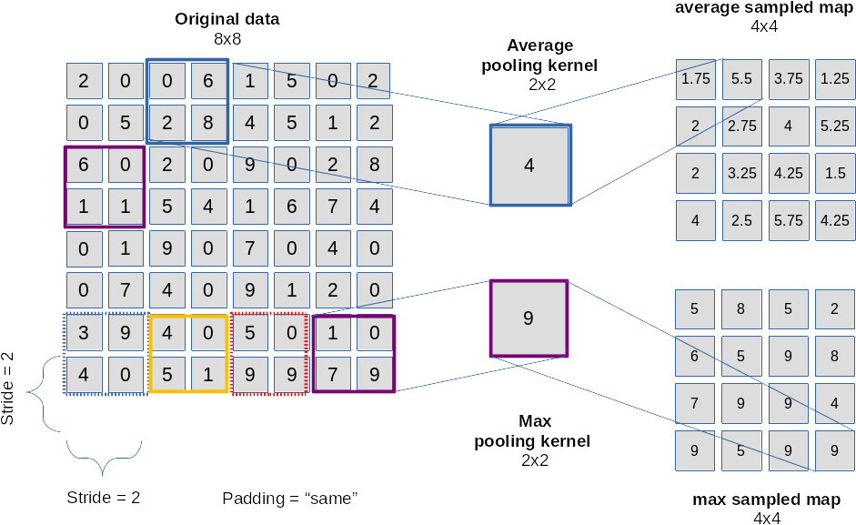
The drawing explains that we “sample” the information over multiple pixels e.g. by
- either calculating an average over pixels (or map node values)
- or by just picking the maximum value of pixels or map node values (thereby stressing the most important information)
in a certain defined sub-area of an image or map.
The shift or stride used as a default in a pooling layer is exactly the side length of the pooling area. We thus cover the image by adjacent, non-overlapping tiles! This leads to a substantial decrease of the dimensions of the resulting map! With a (2×2) pooling size by a an effective factor of 2. (You can change the default pooling stride – but think about the consequences!)
Of course, averaging or picking a max value corresponds to information reduction.
However: What the CNN really also will do in a subsequent Conv layer is to invest in further weights for the combination of information (features) in and of substantially larger areas of the original image! Pooling followed by an additional convolution obviously supports hierarchy building of information on different scales of image areas!
After we first have concentrated on small scale features (like with a magnifying glass) we now – in a figurative sense – make a step backwards and look at larger scales of the image again.
The trick is to evaluate large scale information by sampling layers in addition to the small scale information information already extracted by the previous convolutions. Yes, we drop resolution information – but by introducing a suitable mix of convolutions and sampling layers we also force the network systematically to concentrate on combined large scale features, which in the end are really important for the image classification as a whole!
As sampling counterbalances an explosion of parameters we can invest into a growing number of feature maps with growing scales of covered image areas. I.e. we add more and new filters reacting to combinations of larger scale information.
Look at the second to last illustration: Assume that the 32 maps on layer L_N depicted there are the result of a sampling operation. The next convolution gathers new knowledge about more, namely 64 different combinations of filtered structures over a whole vertical stack of small filter areas located at the same position on the 32 maps of layer N. The new information is in the course of training conserved into 64 weight ensembles for 64 maps on layer N+1.
Resulting options for architectures
We can think of multiple ways of combining Conv layers and pooling layers. A simple recipe for small images could be
- Layer 0: Input layer (tensor of original image data, 3 color layers or one gray layer)
- Layer 1: Conv layer (small 3×3 kernel, stride 1, 32 filters, 32 maps (26×26), analyzes 3×3 overlapping areas)
- Layer 2: Pooling layer (2×2 max pooling => 32 (13×13) maps,
a node covers 4×4 non overlapping areas per node on the original image)
- Layer 3: Conv layer (3×3 kernel, stride 1, 64 filters, 64 maps (11×11),
a node covers 8×8 overlapping areas on the original image (total effective stride 2))
- Layer 4: Pooling layer (2×2 max pooling => 64 maps (5×5),
a node covers 10×10 areas per node on the original image (total effective stride 5), some border info lost)
- Layer 5: Conv layer (3×3 kernel, stride 1, 64 filters, 64 maps (3×3),
a node covers 18×18 per node (effective stride 5), some border info lost )
The following picture illustrates the resulting successive combinations of nodes along one axis of a 28×28 image.
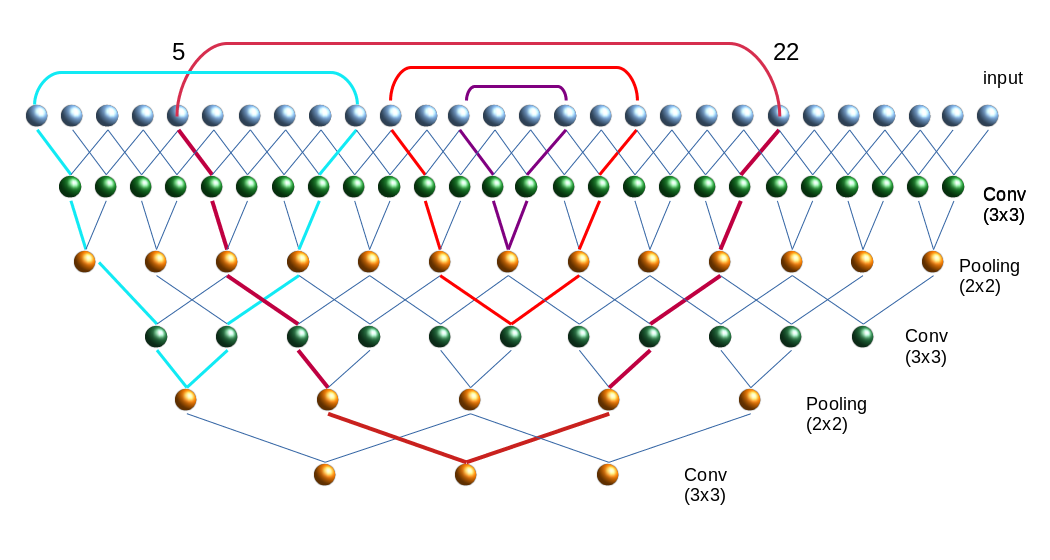
Note that I only indicated the connections to border nodes of the Conv filter areas.
The kernel size decides on the smallest structures we look at – especially via the first convolution. The sampling decides on the sequence of steadily growing areas which we then analyze for specific combinations of smaller structures.
Again: It is most of all the (down-) sampling which allows for an effective hierarchical information building over growing larger image areas! Actually we do not really drop information by sampling – instead we give the network a chance to collect and code new information on a higher, more abstract level (via a whole bunch of numerous new weights).
The big advantages of the sampling layers get obvious:
- They reduce the numbers of required weights
- They reduce the amount of required memory – not only for weights but also for the output data, which must be saved for every layer, map and node.
- They reduce the CPU load for FW and BW propagation
- They also limit the risk of overfitting as some detail information is dropped.
Of course there are many other sequences of layers one could think about. E.g., we could combine 2 to 3 Conv layers before we apply a pooling layer. Such a layer sequence is characteristic of the VGG nets.
Further aspects
Just as MLPs a CNN represents an acyclic graph, where the maps contain increasingly fewer nodes but where the number of maps per layer increases on average.
Questions and objectives for this article series
An interesting question, which seldom is answered in introductory books, is whether two totally independent training runs for a given CNN-architecture applied on the same input data will produce the same filters in the same order. We shall investigate this point in the forthcoming articles.
Another interesting point is: What does a CNN see at which convolution layer?
And even more important: What do the “features” (= basic structural elements) in an image which trigger/activate a specific filter or map, look like?
If we could look into the output at some maps we could possibly see what filters do with the original image. And if we found a way to construct a structured image which triggers a specific filter then we could better understand what patterns the CNN reacts to. Are these patterns really “features” in the sense of conceptual entities? Examples for these different types of visualizations with respect to convolution in a CNN are objectives of this article series.
Conclusion
Today we covered a lot of “theory” on some aspects of CNNs. But we have a sufficiently solid basis regarding the structure and architecture now.
CNNs obviously have a much more complex structure than MLPs: They are deep in the sense of many sequential layers. And each convolutional layer has a complex structure in form of many parallel sub-layers (feature maps) itself. Feature maps are associated with filters, whose parameters (weights) get learned during the training. A map results from covering the original image or a map of a previous layer with small (overlapping) tiles of small filtering areas.
A mix of convolution and pooling layers allows for a look at detail patterns of the image in small areas in lower layers, whilst later layers can focus on feature combinations of larger image areas. The involved filters thus allow for the “awareness” of a hierarchy of features with translational invariance.
Pooling layers are important because they help to control the amount of weight parameters – and they enhance the effectiveness of detecting the most important feature correlations on larger image scales.
All nice and convincing – but the attentive reader will ask: Where and how do we do the classification?
Try to answer this question yourself first.
In the next article we shall build a concrete CNN and apply it to the MNIST dataset of images of handwritten digits. And whilst we do it I deliver the answer to the question posed above. Stay tuned …
Literature
“Advanced Machine Learning with Python”, John Hearty, 2016, Packt Publishing – See chapter 4.
“Deep Learning mit Python und Keras”, Francois Chollet, 2018, mitp Verlag – See chapter 5.
“Hands-On Machine learning with SciKit-Learn, Keras & Tensorflow”, 2nd edition, Aurelien Geron, 2019, O’Reilly – See chapter 14.
“Deep Learning mit Tensorflow, keras und Tensorflow.js”, Matthieu Deru, Alassane Ndiaye, 2019, Rheinwerk Verlag, Bonn – see chapter 3
Further articles in this series
A simple CNN for the MNIST dataset – XI – Python code for filter visualization and OIP detection
A simple CNN for the MNIST dataset – X – filling some gaps in filter
visualization
A simple CNN for the MNIST dataset – IX – filter visualization at a convolutional layer
A simple CNN for the MNIST dataset – VIII – filters and features – Python code to visualize patterns which activate a map strongly
A simple CNN for the MNIST dataset – VII – outline of steps to visualize image patterns which trigger filter maps
A simple CNN for the MNIST dataset – VI – classification by activation patterns and the role of the CNN’s MLP part
A simple CNN for the MNIST dataset – V – about the difference of activation patterns and features
A simple CNN for the MNIST dataset – IV – Visualizing the activation output of convolutional layers and maps
A simple CNN for the MNIST dataset – III – inclusion of a learning-rate scheduler, momentum and a L2-regularizer
A simple CNN for the MNIST datasets – II – building the CNN with Keras and a first test
A simple CNN for the MNIST datasets – I – CNN basics
Addendum 20.10.2020: “Feature maps” or “response maps”?
Whilst reading some more books on AI I got the impression that some authors associate the term “feature map” with the full collection of all maps related to a Conv layer. A single map then is called a “response map” or an “output channel” of the feature map. However, as most books (e.g. the book of A. Geron on Machine Learning) call a singular map a “feature map” I cling to this usage throughout this series.