This brief article continues my series on a Python program for simple MLPs.

With the code for “Error Backward Propagation” we have come so far that we can perform first tests. As planned from the beginning we take the MNIST dataset as a test example. In a first approach we do not rebuild the mini-batches with each epoch. Neither do we vary the MLP setup.

What we are interested in is the question whether our artificial neural network converges with respect to final weight values during training. I.e. we want to see whether the training algorithm finds a reasonable global minimum on the cost hyperplane over the parameter space of all weights.

Test results

We use the following parameters

    ANN = myann.MyANN(my_data_set="mnist_keras", n_hidden_layers = 2, 
                 ay_nodes_layers = [0, 70, 30, 0], 
                 n_nodes_layer_out = 10,  

                 #my_loss_function = "MSE",
                 my_loss_function = "LogLoss",
                 n_size_mini_batch = 500,
     
                 n_epochs = 1500, 
                 n_max_batches = 2000,
                     
                 lambda2_reg = 0.1, 
                 lambda1_reg = 0.0,      

                 vect_mode = 'cols', 
                      
                 learn_rate = 0.0001,
                 decrease_const = 0.000001,
                 mom_rate   = 0.00005,  

                 figs_x1=12.0, figs_x2=8.0, 
                 legend_loc='upper right',
                 b_print_test_data = True
                 )

We use two hidden layers with 70 and 30 nodes. Note that we pick a rather small learning rate, which gets diminished even further. The number of epochs (1500) is quite high; with 4 CPU threads on an i7-6700K processor training takes around 40 minutes if started from a Jupyter notebook. (Our program is not yet optimized.)

I supplemented my code with some statements to print out data for the total costs and the averaged error for mini-batches. We get the
following series of data for the last mini-batch within every 50th epoch.

Starting epoch 1
total costs of mini_batch =  1757.1499806500506
avg total error of mini_batch =  0.17150838451718683
---------
Starting epoch 51
total costs of mini_batch =  532.5817607913532
avg total error of mini_batch =  0.034658195573307196
---------
Starting epoch 101
total costs of mini_batch =  436.67115522484687
avg total error of mini_batch =  0.023496458964699055
---------
Starting epoch 151
total costs of mini_batch =  402.381331415108
avg total error of mini_batch =  0.020836159866695597
---------
Starting epoch 201
total costs of mini_batch =  342.6296325512483
avg total error of mini_batch =  0.016565121882126693
---------
Starting epoch 251
total costs of mini_batch =  319.5995117831668
avg total error of mini_batch =  0.01533372596379799
---------
Starting epoch 301
total costs of mini_batch =  288.2201307002896
avg total error of mini_batch =  0.013799141451102469
---------
Starting epoch 351
total costs of mini_batch =  272.40526022720826
avg total error of mini_batch =  0.013499221607285198
---------
Starting epoch 401
total costs of mini_batch =  251.02417188663628
avg total error of mini_batch =  0.012696943309314687
---------
Starting epoch 451
total costs of mini_batch =  231.92274565746214
avg total error of mini_batch =  0.011152542115360705
---------
Starting epoch 501
total costs of mini_batch =  216.34658280101385
avg total error of mini_batch =  0.010692239864121407
---------
Starting epoch 551
total costs of mini_batch =  215.21791509166042
avg total error of mini_batch =  0.010999255316821901
---------
Starting epoch 601
total costs of mini_batch =  207.79645393570436
avg total error of mini_batch =  0.011123079894527222
---------
Starting epoch 651
total costs of mini_batch =  188.33965068903723
avg total error of mini_batch =  0.009868734062493835
---------
Starting epoch 701
total costs of mini_batch =  173.07625091642274
avg total error of mini_batch =  0.008942065167336382
---------
Starting epoch 751
total costs of mini_batch =  174.98264336120369
avg total error of mini_batch =  0.009714870291761567
---------
Starting epoch 801
total costs of mini_batch =  161.10229359519792
avg total error of mini_batch =  0.008844419847237179
---------
Starting epoch 851
total costs of mini_batch =  155.4186141788981
avg total error of mini_batch =  0.008244783820578621
---------
Starting epoch 901
total costs of mini_batch =  158.88876607392308
avg total error of mini_batch =  0.008970678691005138
---------
Starting epoch 951
total costs of mini_batch =  148.61870772570722
avg total error of mini_batch =  0.008124438423034456
---------
Starting epoch 1001
total costs of mini_batch =  152.16976618516264
avg total error of mini_batch =  0.009151413825781066
---------
Starting epoch 1051
total costs of mini_batch =  142.24802525081637
avg total error of mini_batch =  0.008297161160449798
---------
Starting epoch 1101
total costs of mini_batch =  137.3828515603569
avg total error of mini_batch =  0.007659755348989629
---------
Starting epoch 1151
total costs of mini_batch =  129.8472897084494
avg total error of mini_batch =  0.007254892176613871
---------
Starting epoch 1201
total costs of mini_batch =  139.30002497623792
avg total error of mini_batch =  0.007881199505625214
---------
Starting epoch 1251
total costs of mini_batch =  138.0323454321882
avg total error of mini_batch =  0.00807373439996105
---------
Starting epoch 1301
total costs of mini_batch =  117.95701570484076
avg total error of mini_batch =  0.006378071703153664
---------
Starting epoch 1351
total costs of mini_batch =  125.
71869046937177
avg total error of mini_batch =  0.0072716189968114265
---------
Starting epoch 1401
total costs of mini_batch =  117.3485602627176
avg total error of mini_batch =  0.006291182169676069
---------
Starting epoch 1451
total costs of mini_batch =  118.09317470010767
avg total error of mini_batch =  0.0066519021636054195
---------
Starting epoch 1491
total costs of mini_batch =  112.69566736699439
avg total error of mini_batch =  0.006151660466611035

 ------
Total training Time_CPU:  2430.0504785089997

We can display the results also graphically; a code fragemnt to do this, may look like follows in a Jupyter cell:

# Plotting 
# **********
num_epochs  = ANN._ay_costs.shape[0]
num_batches = ANN._ay_costs.shape[1]
num_tot = num_epochs * num_batches

ANN._ay_costs = ANN._ay_costs.reshape(num_tot)
ANN._ay_theta = ANN._ay_theta .reshape(num_tot)

#sizing
fig_size = plt.rcParams["figure.figsize"]
fig_size[0] = 12
fig_size[1] = 5

# Two figures 
# -----------
fig1 = plt.figure(1)
fig2 = plt.figure(2)

# first figure with two plot-areas with axes 
# --------------------------------------------
ax1_1 = fig1.add_subplot(121)
ax1_2 = fig1.add_subplot(122)

ax1_1.plot(range(len(ANN._ay_costs)), ANN._ay_costs)
ax1_1.set_xlim (0, num_tot+5)
ax1_1.set_ylim (0, 2000)
ax1_1.set_xlabel("epochs * batches (" + str(num_epochs) + " * " + str(num_batches) + " )")
ax1_1.set_ylabel("costs")

ax1_2.plot(range(len(ANN._ay_theta)), ANN._ay_theta)
ax1_2.set_xlim (0, num_tot+5)
ax1_2.set_ylim (0, 0.2)
ax1_2.set_xlabel("epochs * batches (" + str(num_epochs) + " * " + str(num_batches) + " )")
ax1_2.set_ylabel("averaged error")

We get:

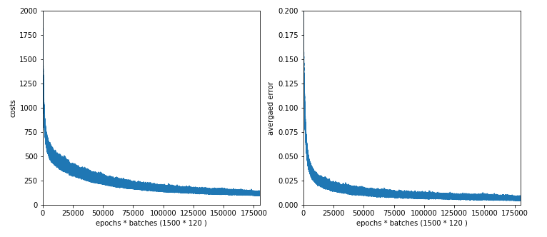
This looks quite promising!
The vertical spread of both curves is due to the fact that we plotted cost and error data for each mini-batch. As we know the cost hyperplanes of the batches differ from each other and the hyperplane of the total costs for all training data. So do the cost and error values.

Secondary test: Rate of correctly and wrongly predicted values of the training and the test data sets

With the following code in a Jupyter cell we can check the relative percentage of correctly predicted MNIST numbers for the training data set and the test data set:

# ------ all training data 
# *************************
size_set = ANN._X_train.shape[0]

li_Z_in_layer_test  = [None] * ANN._n_total_layers
li_Z_in_layer_test[0] = ANN._X_train
# Transpose 
ay_Z_in_0T       = li_Z_in_layer_test[0].T
li_Z_in_layer_test[0] = ay_Z_in_0T
li_A_out_layer_test  = [None] * ANN._n_total_layers

ANN._fw_propagation(li_Z_in = li_Z_in_layer_test, li_A_out = li_A_out_layer_test, b_print = True) 
Result = np.argmax(li_A_out_layer_test[3], axis=0)
Error = ANN._y_train - Result 
acc_train = (np.sum(Error == 0)) / size_set
print ("total accuracy for training data = ", acc_train)

# ------ all test data 
# *************************
size_set = ANN._X_test.shape[0]

li_Z_in_layer_test  = [None] * ANN._n_total_layers
li_Z_in_layer_test[0] = ANN._X_test
# Transpose 
ay_Z_in_0T       = li_Z_in_layer_test[0].T
li_Z_in_layer_test[0] = ay_Z_in_0T
li_A_out_layer_test  = [None] * ANN._n_total_layers

ANN._fw_propagation(li_Z_in = li_Z_in_layer_test, li_A_out = li_A_out_layer_test, b_print = True) 
Result = np.argmax(li_A_out_layer_
test[3], axis=0)
Error = ANN._y_test - Result 
acc_test = (np.sum(Error == 0)) / size_set
print ("total accuracy for test data = ", acc_test)

“acc” stands for “accuracy”.

We get

total accuracy for training data = 0.9919
total accuracy for test data = 0.9645

So, there is some overfitting – but not much.

Conclusion

Our training algorithm and the error backward propagation seem to work.

The real question is, whether we produced the accuracy values really efficiently: In our example case we needed to fix around 786*70 + 70*30 + 30*10 = 57420 weight values. This is close to the total amount of training data (60000). A smaller network with just one hidden layer would require much fewer values – and the training would be much faster regarding CPU time.

So, in the next article
A simple program for an ANN to cover the Mnist dataset – X – mini-batch-shuffling and some more tests
we shall extend our tests to different setups of the MLP.

Linux-Blog – Dr. Mönchmeyer / anracon

Notes about Linux, ML and some simple math …

A simple Python program for an ANN to cover the MNIST dataset – IX – First Tests

Test results

Secondary test: Rate of correctly and wrongly predicted values of the training and the test data sets

Conclusion