I continue with my analysis of the z-point and latent vector distribution a trained Autoencoder creates in its latent space for CelebA images. These images show human faces. To make the Autoencoder produce new face images from statistically generated latent vectors is a problem. See some previous posts in this series for reasons.
Autoencoders and latent space fragmentation – I – Encoder, Decoder, latent space
Autoencoders and latent space fragmentation – II – number distributions of latent vector components
Autoencoders and latent space fragmentation – III – correlations of latent vector components
Autoencoders and latent space fragmentation – IV – CelebA and statistical vector distributions in the surroundings of the latent space origin
Autoencoders and latent space fragmentation – V – reconstruction of human face images from simple statistical z-point-distributions?
These problems are critical for a generative usage of standard Autoencoders. Generative tasks in Machine Learning very often depend on a clear and understandable structure of the latent space regions an Encoder/Decoder pair uses. In general we would like to create statistical latent vectors such that a reasonable object creation (here: image creation) is guaranteed. In the last post
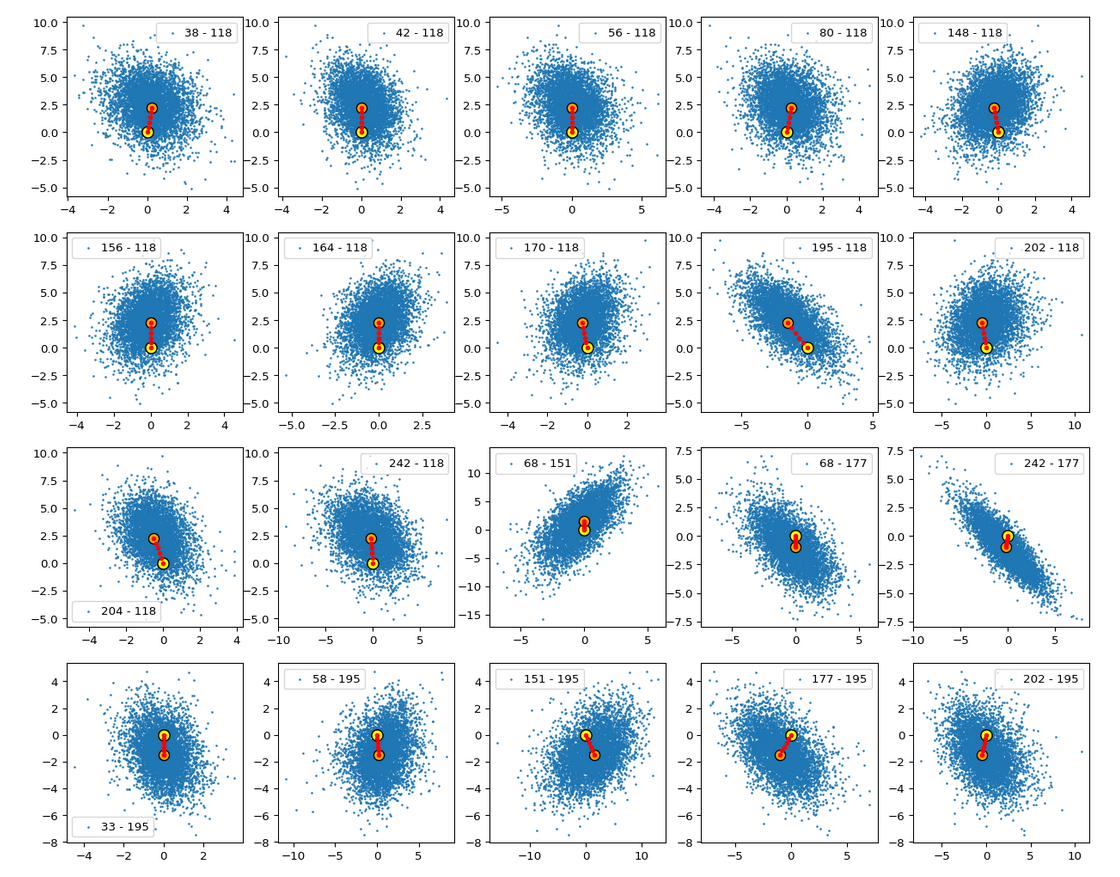
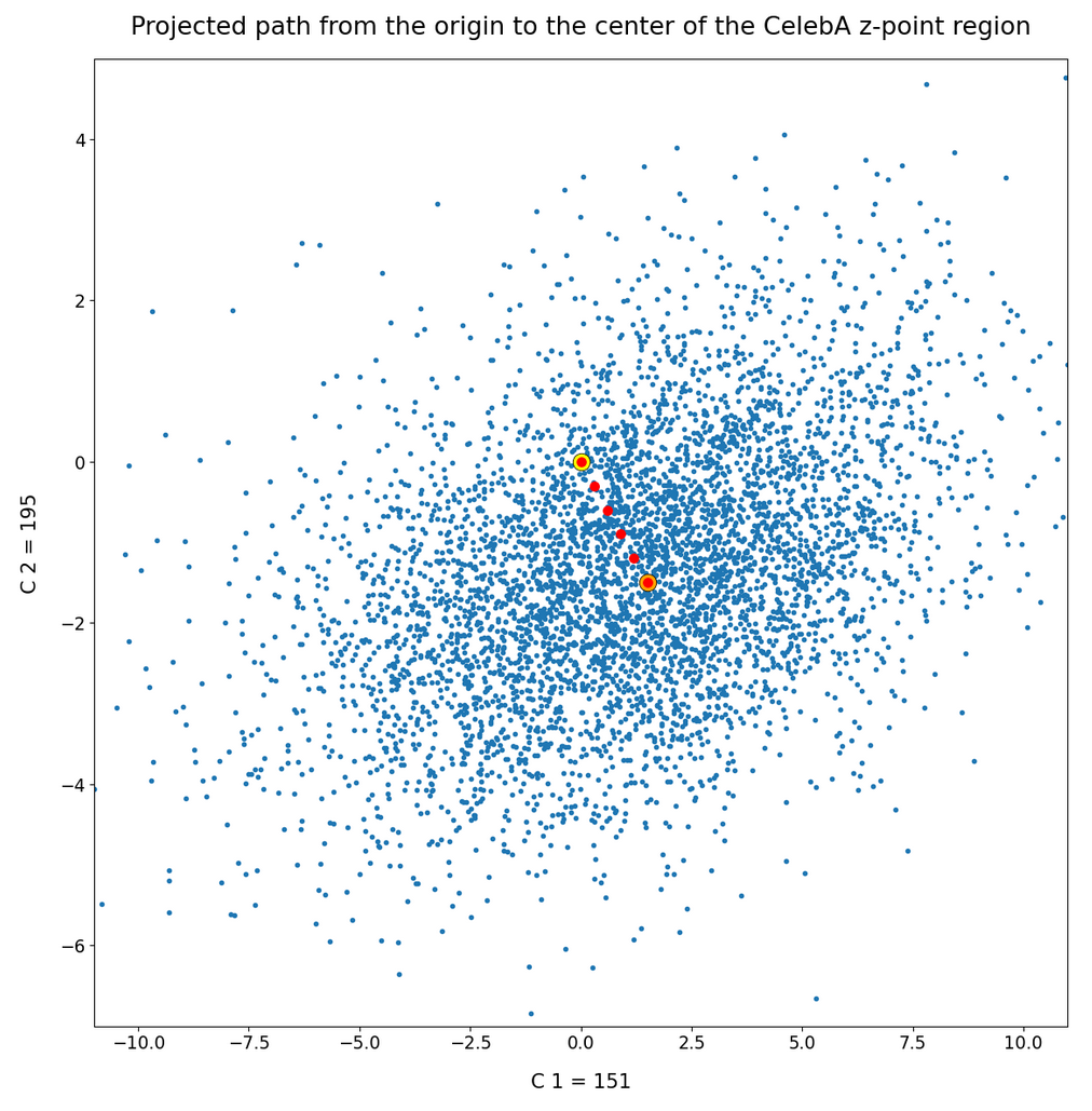
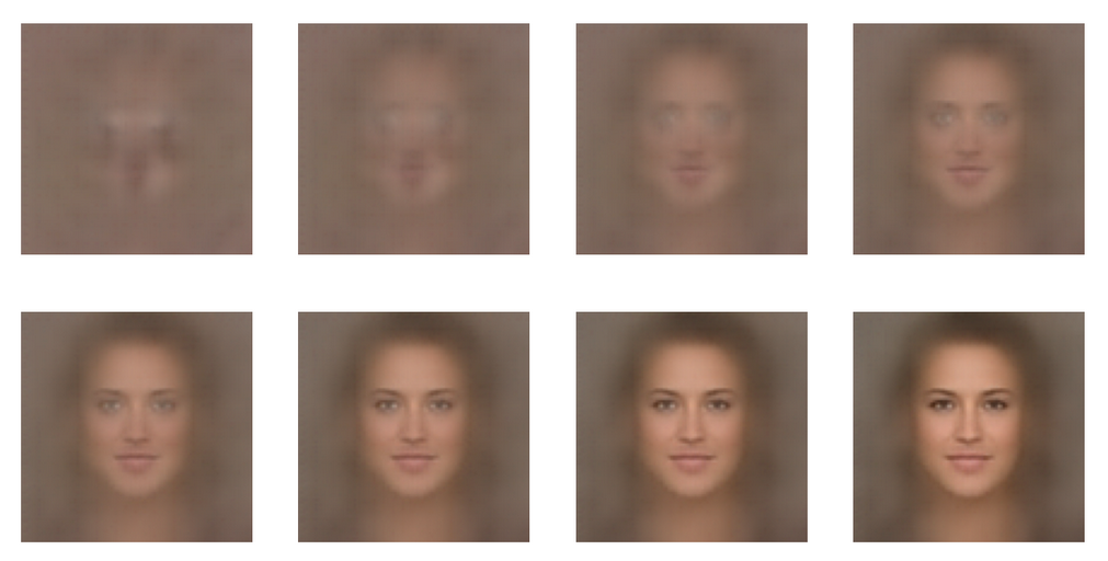
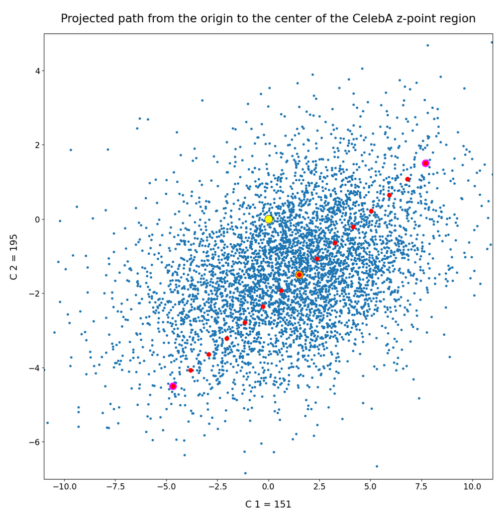
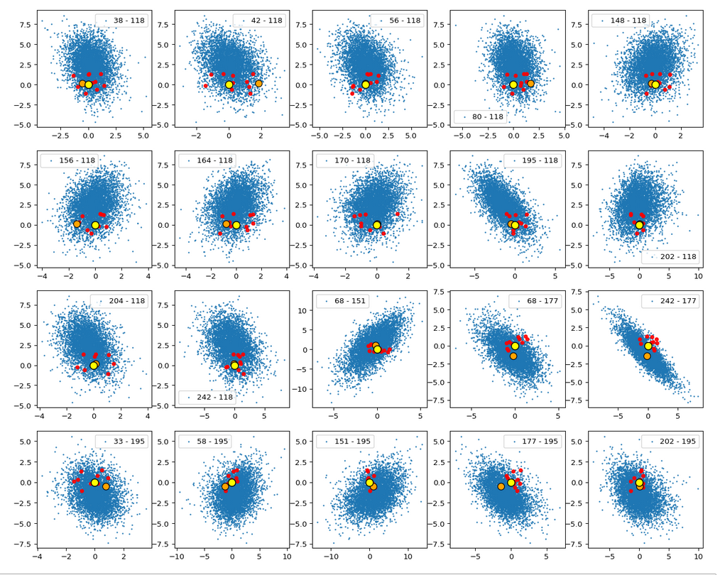
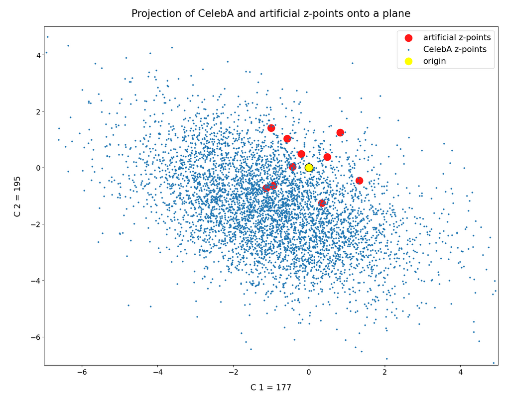
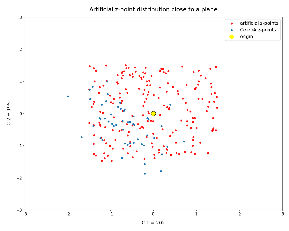
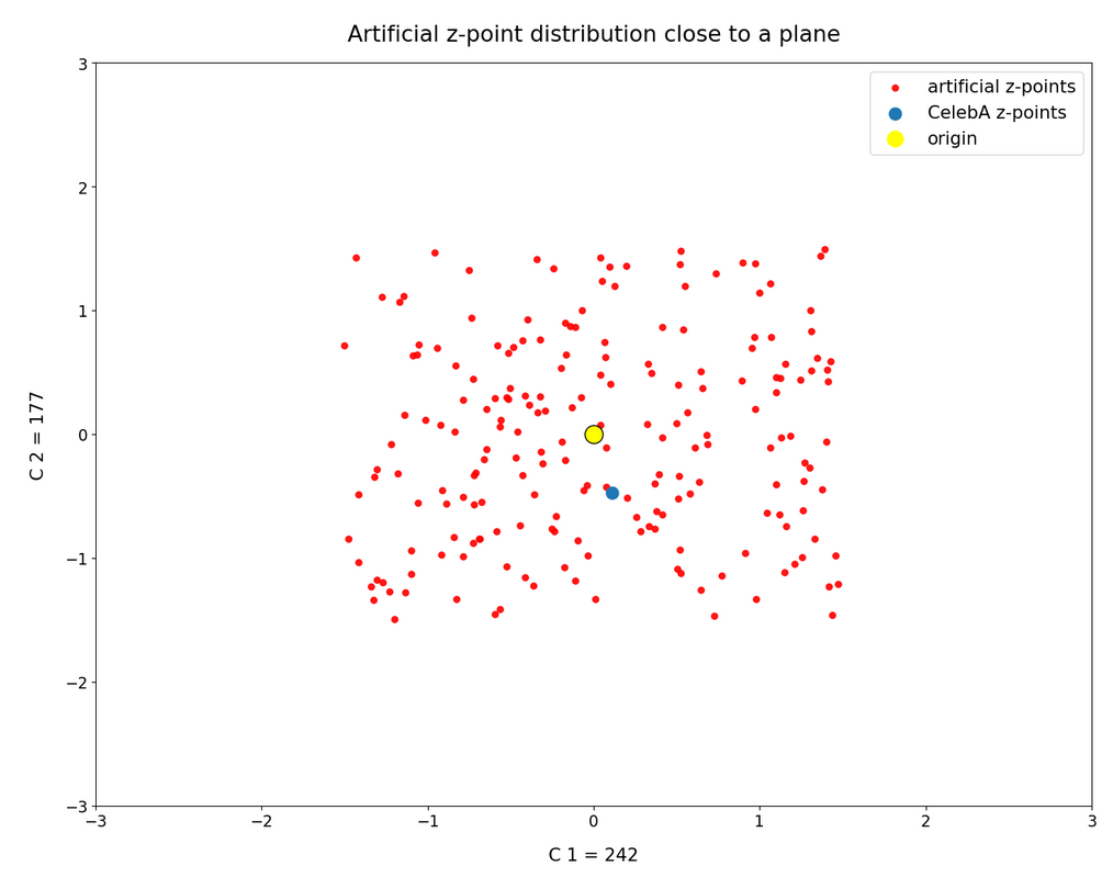
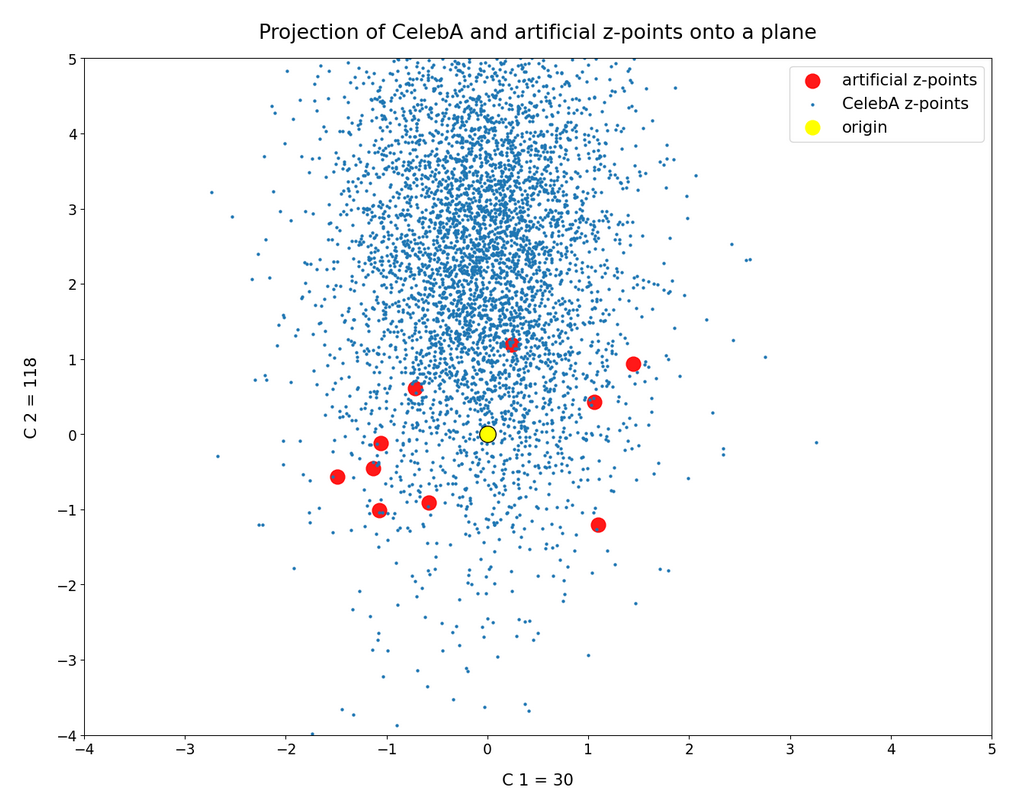
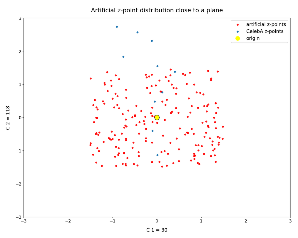
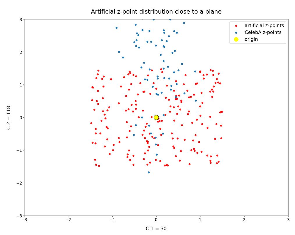
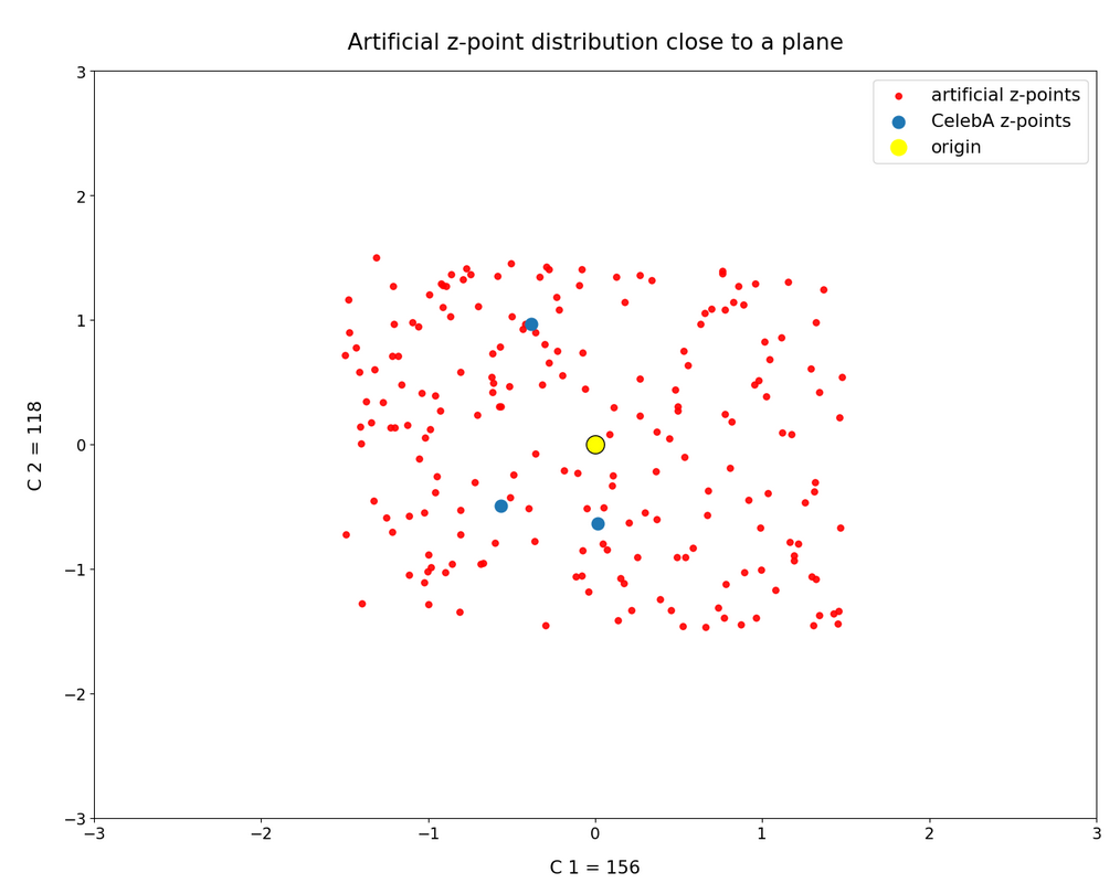
we saw that we at least get some clear face features when we make use of some basic information about the shape and location of the z-point distribution for the images the AE was trained with. This distribution is specific for an Autoencoder, the image set used and details of the training run. In our case the z-point distribution could be analyzed by rather simple methods after the training of an AE with CelebA images had been concluded. The number distribution curves per vector component revealed value limits per latent vector component. The core of the z-point distribution itself appeared to occupy a single and rather compact sub-volume inside the latent space. (The exact properties depend on the AE’s layer structure and the training run.) Of the N=256 dimensions of our latent space only a few determined the off-origin position of the center of the z-point distribution’s core. This multidimensional core had an overall ellipsoidal shape. We could see this both from the Gaussian like number distributions for the components and more directly from projections onto 2-dimensional coordinate planes. (We will have a closer look at these properties which indicate a multivariate normal distribution in forthcoming posts.)
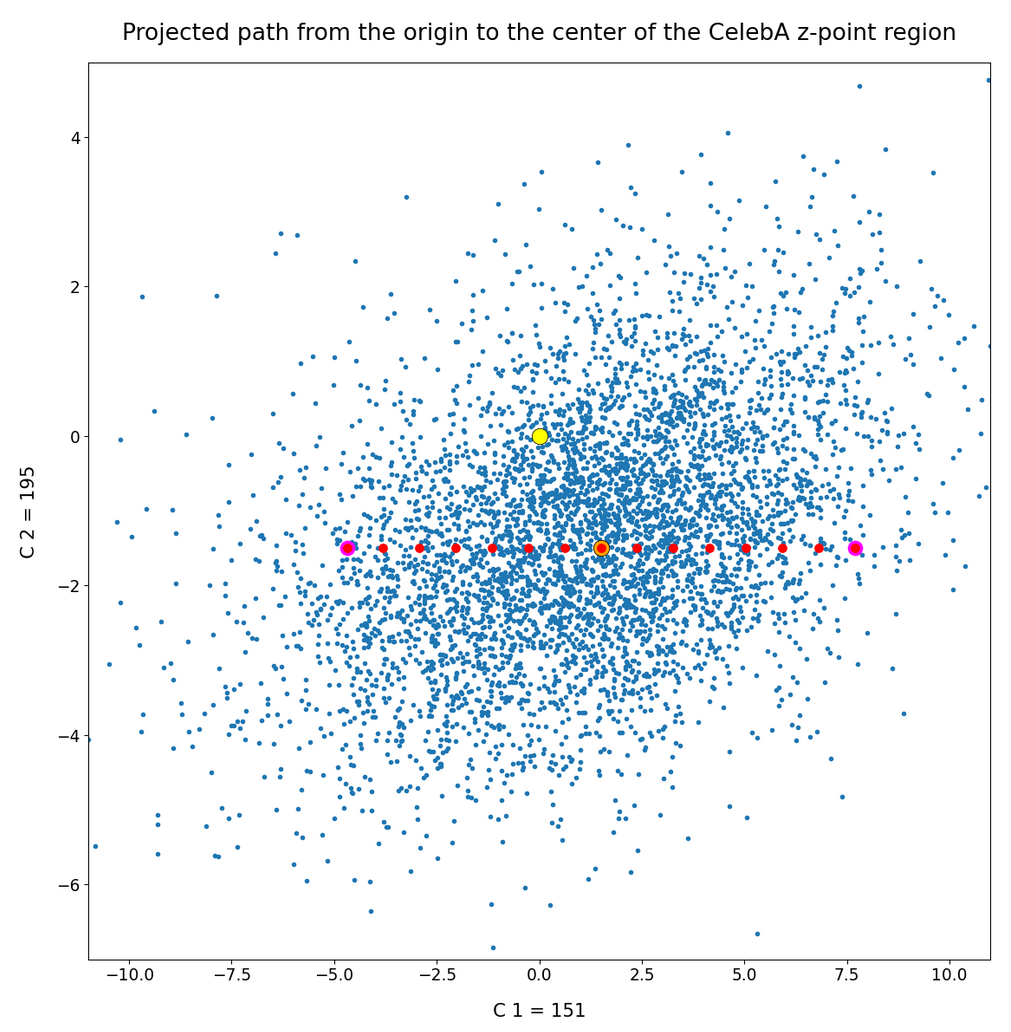
As long as we kept the statistical values for artificial latent vector components within the value ranges set by the distribution’s core our chances that the AE’s Decoder produced images with new and clearly visible faces rose significantly. So far we have only used z-points along defined paths crossing the distributions core. In this post I will vary the components of our statistically created latent vectors a bit more freely. This will again show us that correlations of the vector components are important.
Constant probability for each component value within a component specific interval
In the first posts of this series I naively created statistical latent vectors from a common value range for the components. We saw this was an inadequate approach – both for general mathematical and for problem specific reasons. The following code snippets shows an approach which takes into account value ranges coming from the Gaussian-like distributions for the individual components of the latent vectors for CelebA. The arrays “ay_mu_comp” and “ay_mu_hw” have the following meaning:
- ay_mu_comp: Component values of a latent vector pointing to the center of the CelebA related z-point distribution
- ay_mu_hw: Half-width of the Gaussian like number distribution for the component specific values
num_per_row  = 7
num_rows     = 3
num_examples = num_per_row * num_rows

fact = 1.0

# Get component specific value ranges into an array
li_b = []
for j in range(0, z_dim):
    add_val = fact*abs(ay_mu_hw[j])
    b_l = ay_mu_comp[j] - add_val
    b_r = ay_mu_comp[j] + add_val
    li_b.append((b_l, b_r))

# Statistical latent vectors
ay_stat_zpts = np.zeros( (num_examples, z_dim), dtype=np.float32 )
for i in range(0, num_examples):
    for j in range(0, z_dim):
        b_l = li_b[j][0]
        b_r = li_b[j][1]
        val_c = np.random.uniform(b_l, b_r)
        ay_stat_zpts[i, j] = val_c

# Prediction
reco_img_stat = AE.decoder.predict(ay_stat_zpts)
# print("Shape of reco_img = ", reco_img_stat.shape)
The main difference is that we take random values from real value intervals defined per component. Within each interval we assume a constant probability density. The factor “fact” controls the width of the value interval we use. A small value covers the vicinity of the center of the CelebA z-point distribution; a larger fact leads to values at the border region of the z-point distribution.
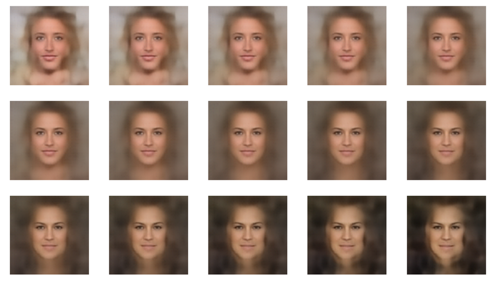
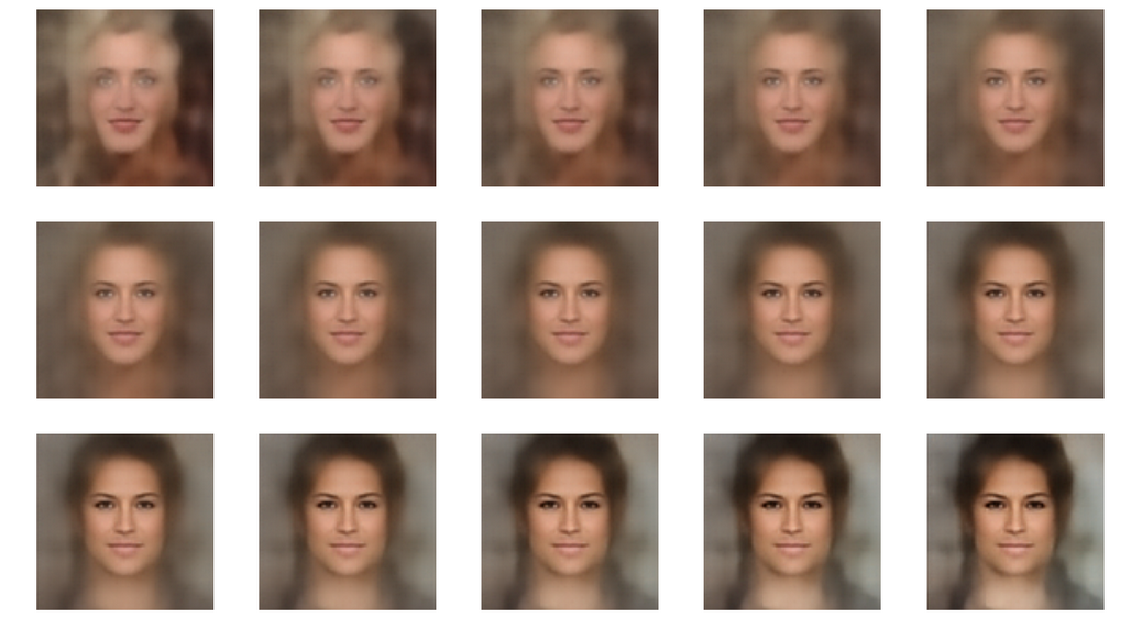
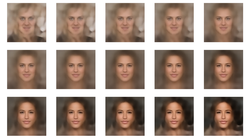
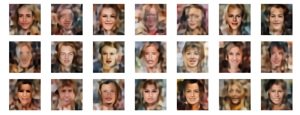
Image results for different value ranges
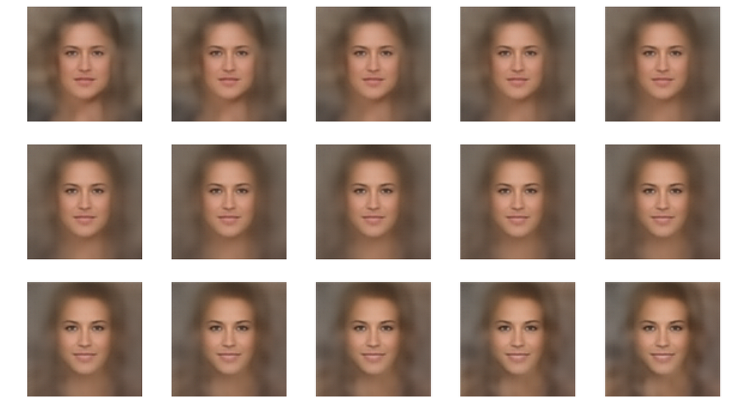
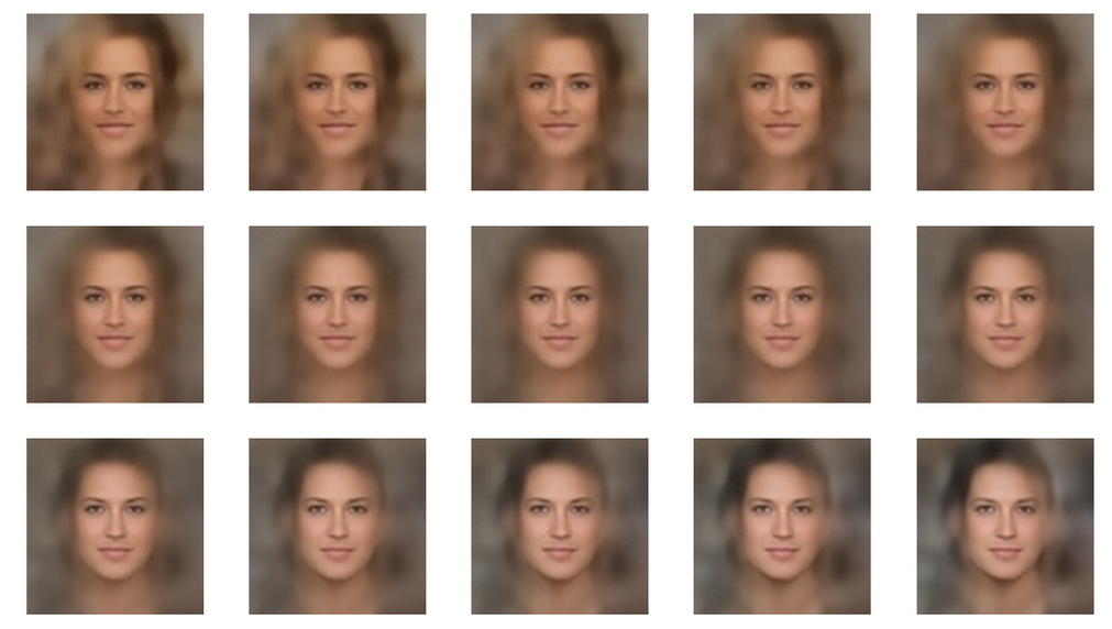
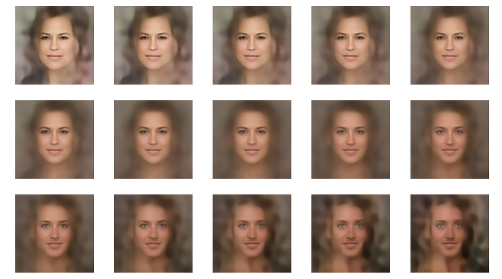
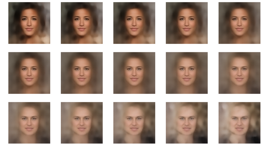
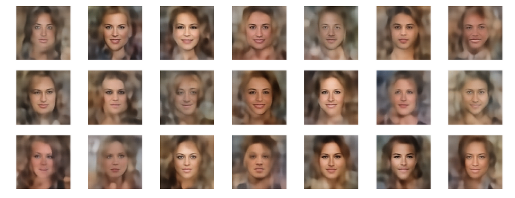
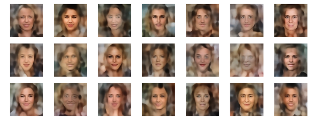
fact=0.4
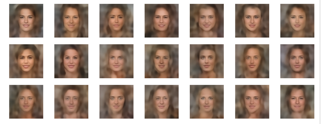
fact=0.5
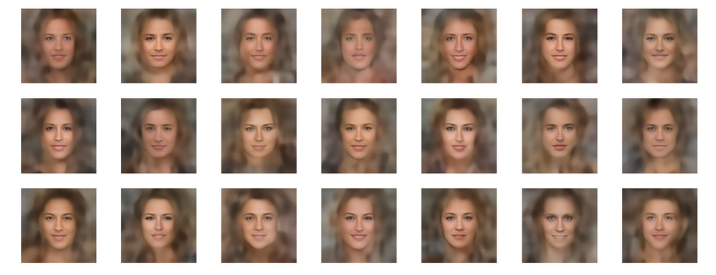
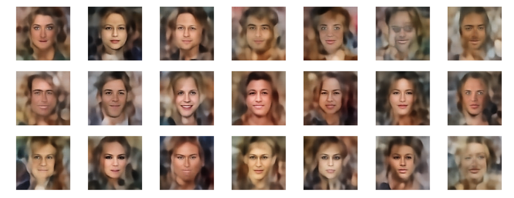
fact=0.6
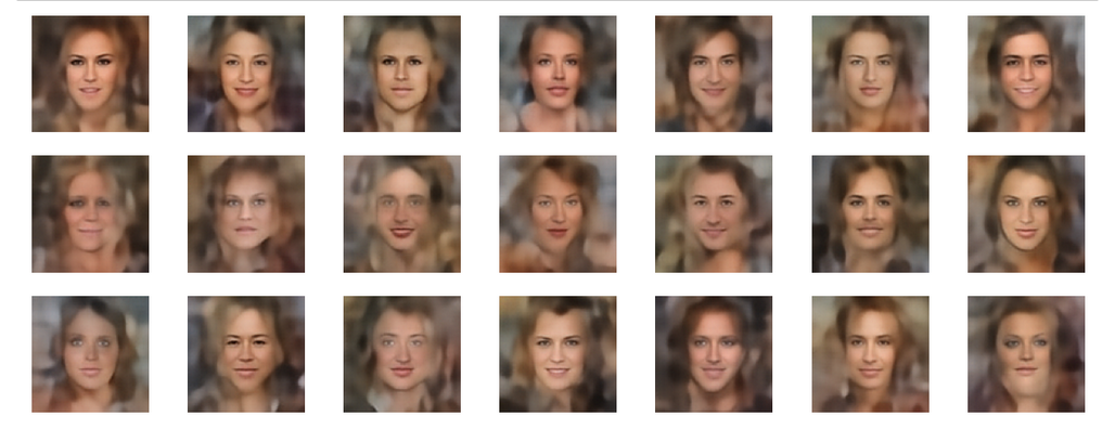
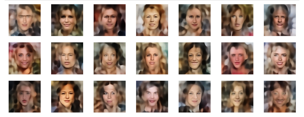
fact=0.7
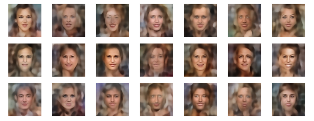
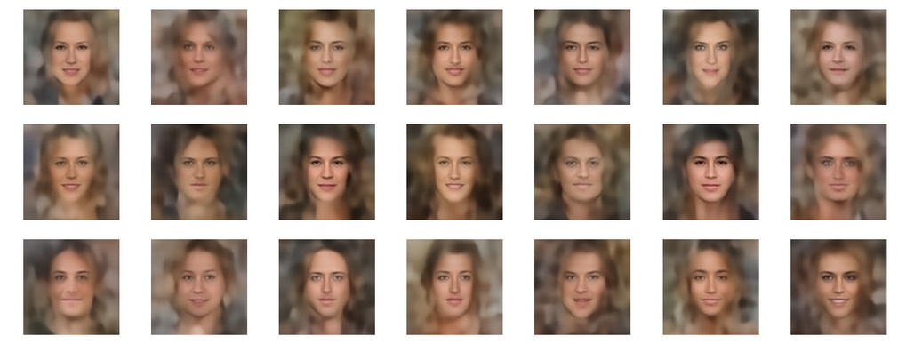
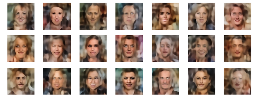
fact=0.8
fact=0.9
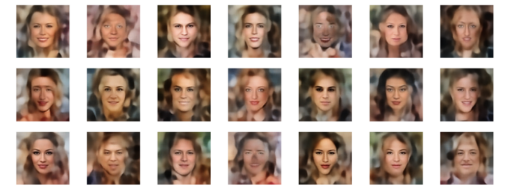
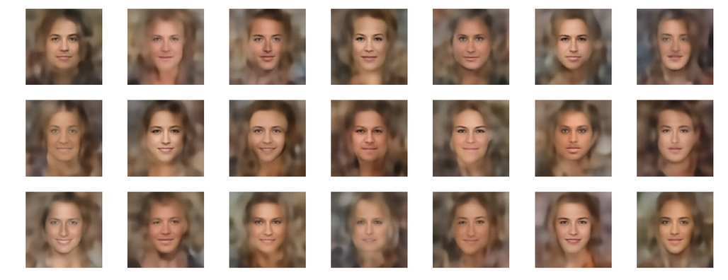
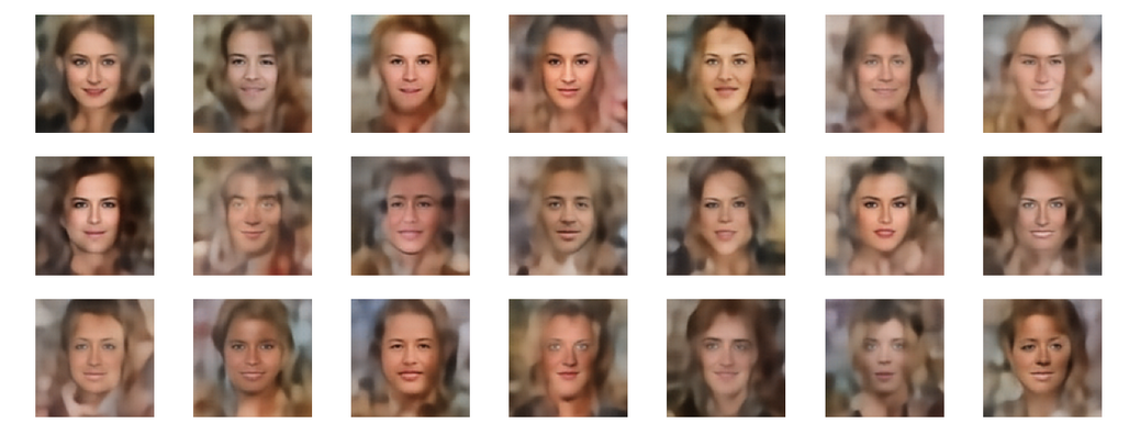
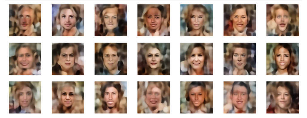
fact=1.0
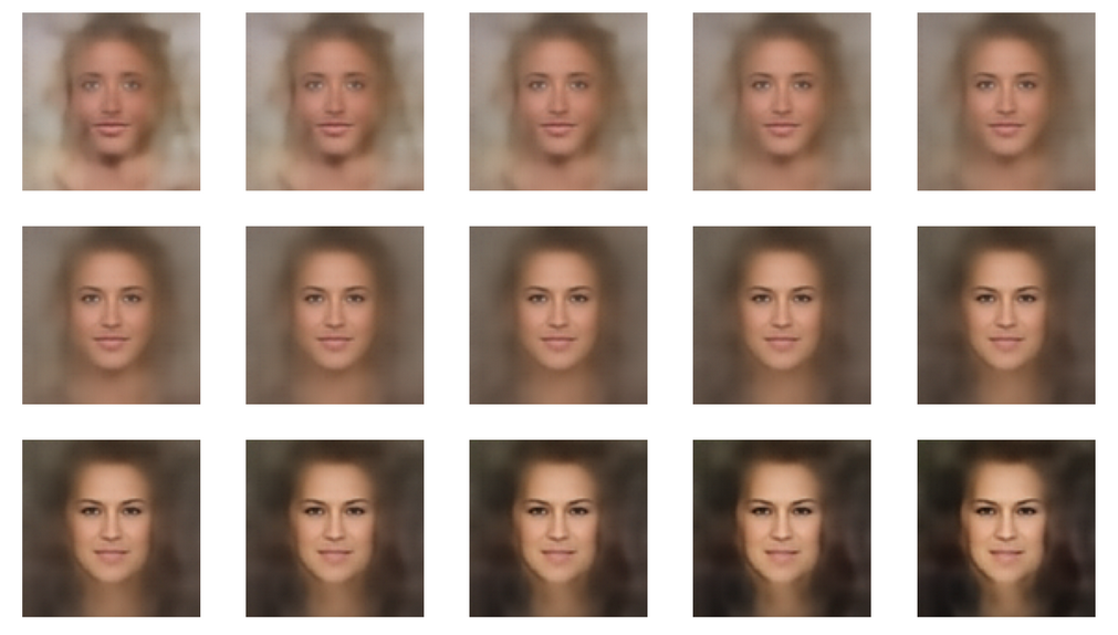
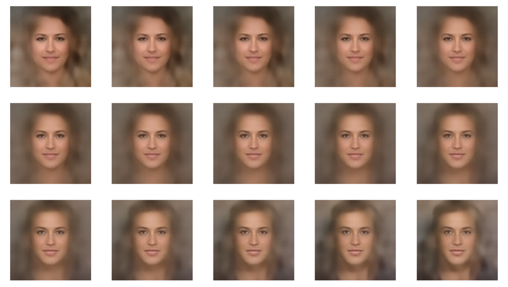
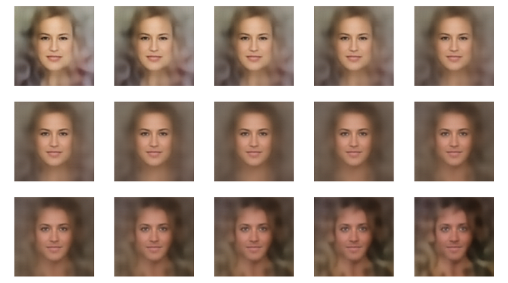
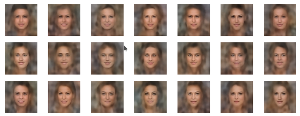
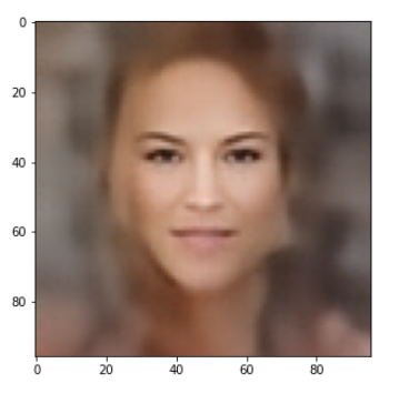
Selected individuals
Below you find some individual images created for a variety of statistical vectors. They are ordered by a growing distance from the center of the CelebA related z-point distribution.
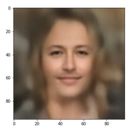
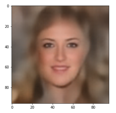
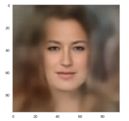

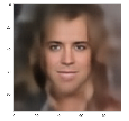

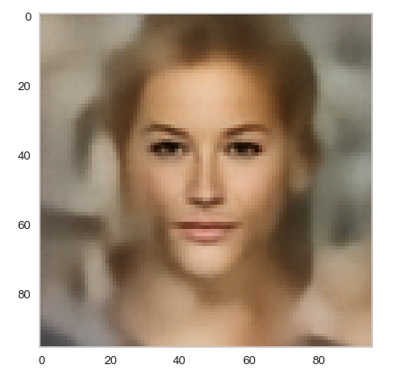

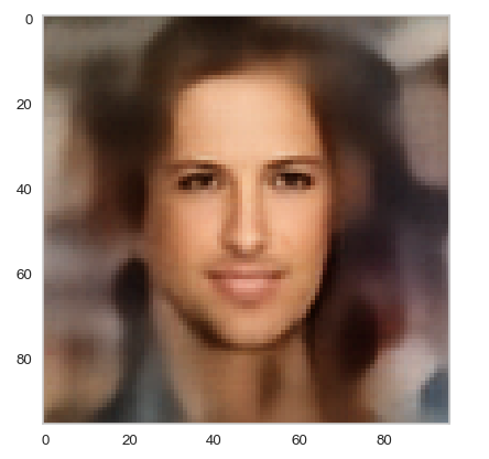

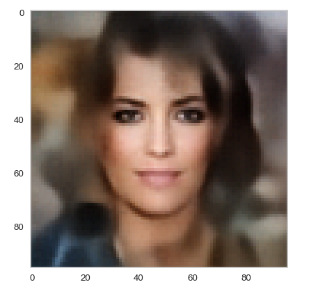
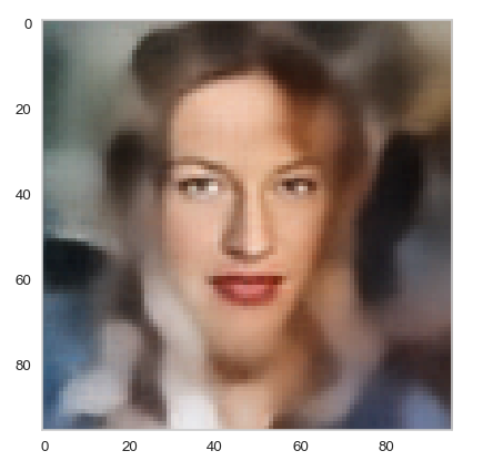
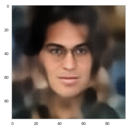
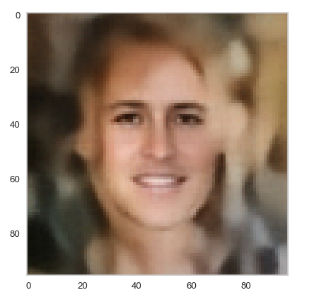
Quality? Missing correlations?
The first thing we see is that we get problems for all factors fact. Some images are OK, but others show disturbances and the contrasts of the face against the background are not well defined – even for small factors fact. The reason is that our random selection ignores correlations between the components completely. But we know already that there are major correlations between certain vector components.
For larger values of fact the risk to place a generated latent vector outside the core of the CelebA z-point distribution gets bigger. Still some images interesting face variations.
Obviously, we have no control over the transitions from face to hair and from hair to background. Our suspicion is that micro-correlations of the latent vector components for CelebA images may encode the respective information. To understand this aspect we would have to investigate the vicinity of a z-point a bit more in detail.
Conclusion
We are able to create images with new human faces by using statistical latent vectors whose component values fall into component specific defined real value intervals. We can derive the limits of these value ranges from the real z-point distribution for CelebA images of a trained AE. But again we saw:
One should not ignore major correlations between the component values.
We have to take better care of this point in a future post when we perform a transformation of the coordinate system to align with the main axes of the z-point distribution. But there is another aspect which is interesting, too:
Micro-correlations between latent vector components may determine the transition from faces to complex hair and background-patterns.
We can understand such component dependencies when we assume that the superposition especially of small scale patterns a convolutional Decoder must arrange during image creation is a subtle balancing act. A first step to understand such micro-correlations better could be to have a closer look at the nearest CelebA z-point neighbors of an artificially created latent z-point. If they form some kind of pattern, then maybe we can change the components of our z-point a bit in the right direction?
Or do we have to deal with correlations on a much coarser level? What do the Gaussians and the roughly elliptic form of the core of the z-point distribution for CelebA images really imply? This is the topic of the next post.