The topics of this post series are
- convolutional Autoencoders,
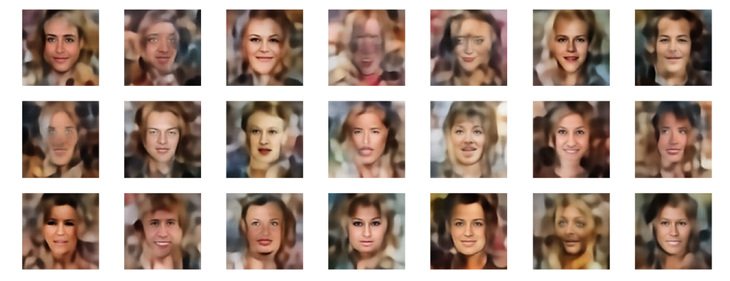
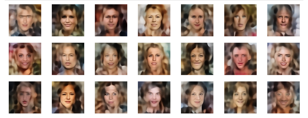
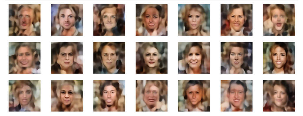
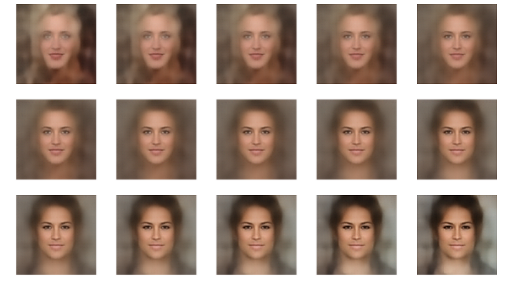
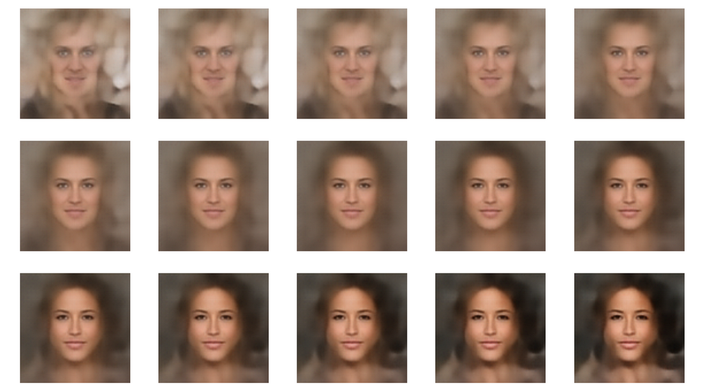
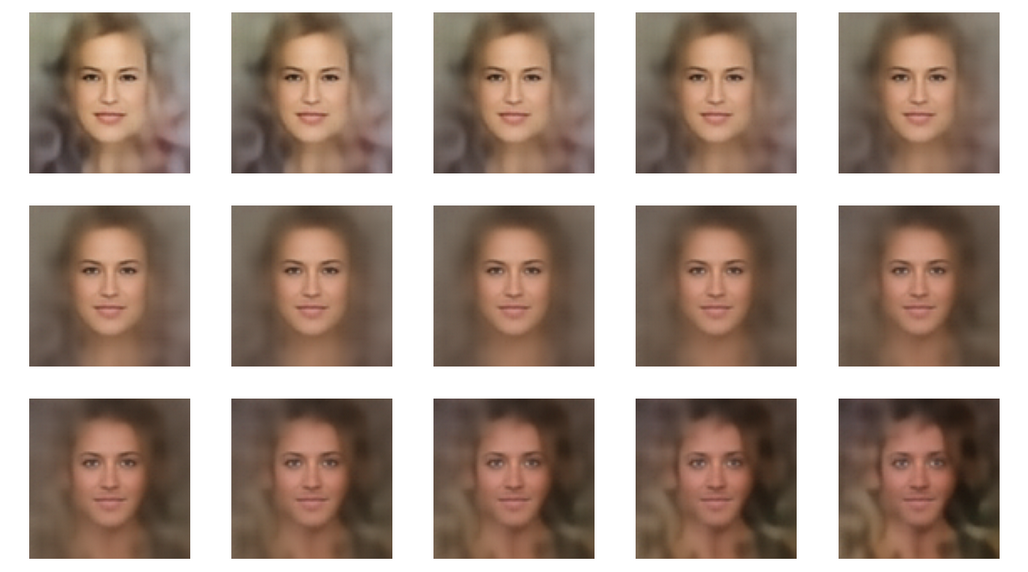
- images of human faces, provided by the CelebA dataset
- and related data point and vector distributions in the AEs’ latent spaces.
In the first post
Autoencoders and latent space fragmentation – I – Encoder, Decoder, latent space
I have repeated some basics about the representation of images by vectors. An image corresponds e.g. to a vector in a feature space with orthogonal axes for all individual pixel values. An AE’s Encoder compresses and encodes the image information in form of a vector in the AE’s latent space. This space has many, but significantly fewer dimensions than the original feature space. The end-points of latent vectors are so called z-points in the latent space. We can plot their positions with respect to two coordinate axes in the plane spanned by these axes. The positions reflect the respective vector component values and are the result of an orthogonal projection of the z-points onto this plane. In the second post
Autoencoders and latent space fragmentation – II – number distributions of latent vector components
I have discussed that the length and orientation of a latent vector correspond to a recipe for a constructive process of The AE’s (convolutional) Decoder: The vector component values tell the Decoder how to build a superposition of elementary patterns to reconstruct an image in the original feature space. The fundamental patterns detected by the convolutional AE layers in images of the same class of objects reflect typical pixel correlations. Therefore the resulting latent vectors should not vary arbitrarily in their orientation and length.
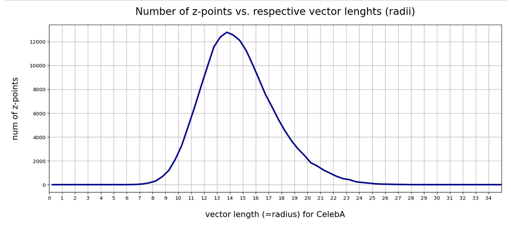
By an analysis of the component values of the latent vectors for many CelebA images we could explicitly show that such vectors indeed have end points within a small coherent, confined and ellipsoidal region in the latent space. The number distributions of the vectors’ component values are very similar to Gaussian functions. Most of them with a small standard deviation around a central mean value very close to zero. But we also found a few dominant components with a wider value spread and a central average value different from zero. The center of the latent space region for CelebA images thus lies at some distance from the origin of the latent space’s coordinate system. The center is located close to or within a region spanned by only a few coordinate axes. The Gaussians define a multidimensional ellipsoidal volume with major anisotropic extensions only along a few primary axes.
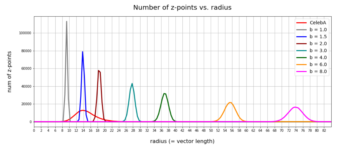
In addition we studied artificial statistical vector distributions which we created with the help of a constant probability distribution for the values of each of the vector components. We found that the resulting z-points of such vectors most often are not located inside the small ellipsoidal region marked by the latent vectors for the CelebA dataset. Due to the mathematical properties of this kind of artificial statistical vectors only rather small parameter values 1.0 ≤ b ≤ 2.0 for the interval [-b, b], from which we pick all the the component values, allow for vectors with at least the right length. However, whether the orientations of such artificial vectors fit the real CelebA vector distribution also depends on possible correlations of the components.
In this post I will show you that there indeed are significant correlations between the components of latent vectors for CelebA images. The correlations are most significant for those components which determine the location of the center of the z-point distribution and the orientation of the main axes of the z-point region for CelebA images. Therefore, a method for statistical vector creation which explicitly treats the vector components as statistically independent properties may fail to cover the interesting latent space region.
Normalized correlation coefficient matrix
When we have N variables (X_1, x_2, … x_n) and M parallel observations for the variable values then we can determine possible correlations by calculating the so called covariance matrix with elements Cij. A normalized version of this matrix provides the so called “Pearson product-moment correlation coefficients” with values in the range [0.0, 1.0]. Values close to 1.0 indicate a significant correlation of the variables x_i and x_j. For more information see e.g. the following links to the documentation on Numpy’s versions for the calculation of the (normalized) covariance matrix from an array containing the observations in an ordered matrix form: “numpy.cov” and to “numpy.corrcoef“.
So what are the “variables” and “observations” in our case?
Latent vectors and their components
In the last post we have calculated the latent vectors that a trained convolutional AE produces for a 170,000 images of the CelebA dataset. As we chose the number N of dimensions of the latent space to be N=256 each of the latent vectors had 256 components. We can interpret the 256 components as our “variables” and the latent vectors themselves as “observations”. An array containing M rows for individual vectors and N columns for the component values can thus be used as input for Numpy’s algorithm to calculate the normalized correlation coefficients.
When you try to perform the actual calculations you will soon detect that determining the covariance values based on a statistics for all of the 170,000 latent vectors which we created for CelebA images requires an enormous amount of RAM with growing M. So, we have to chose M << 170,000. In the calculations below I took M = 5000 statistically selected vectors out of my 170,000 training vectors.
Some special latent vector components
Before I give you the Pearson coefficients I want to remind you of some special components of the CelebA latent vectors. I had called these components the dominant ones as they had either relatively large absolute mean values or a relatively large half-width. The indices of these components, the related mean values mu and half-widths hw are listed below for a AE with filter numbers in the Encoder’s and Decoder’s 4 convolutional layers given by (64, 64, 128, 128) and (128, 128, 64, 64), respectively:
 15   mu : -0.25 :: hw:  1.5
 16   mu :  0.5  :: hw:  1.125
 56   mu :  0.0  :: hw:  1.625
 58   mu :  0.25 :: hw:  2.125
 66   mu :  0.25 :: hw:  1.5
 68   mu :  0.0  :: hw:  2.0
110   mu :  0.5  :: hw:  1.875
118   mu :  2.25 :: hw:  2.25
151   mu :  1.5  :: hw:  4.125
177   mu : -1.0  :: hw:  2.25
178   mu :  0.5  :: hw:  1.875
180   mu : -0.25 :: hw:  1.5
188   mu :  0.25 :: hw:  1.75
195   mu : -1.5  :: hw:  2.0
202   mu : -0.5  :: hw:  2.25
204   mu : -0.5  :: hw:  1.25
210   mu :  0.0  :: hw:  1.75
230   mu :  0.25 :: hw:  1.5
242   mu : -0.25 :: hw:  2.375
253   mu : -0.5  :: hw:  1.0
The first row provides the component number.
Pearson correlation coefficients for dominant components of latent CelebA vectors
For the latent space of our AE we had chosen the number N of its dimensions to be N=256. Therefore, the covariance matrix has 256×256 elements. I do not want to bore you with a big matrix having only a few elements with a size worth mentioning. Instead I give you a code snippet which should make it clear what I have done:
import numpy as np
#np.set_printoptions(threshold=sys.maxsize)

# The Pearson correlation coefficient matrix
# ~~~~~~~~~~~~~~~~~~~~~~~~~~~~~~~~~~~~~~~~~~~~~~
print(z_points.shape)
print()
num_pts      = 5000

# Special points in slice
num_pts_spec = 100000
jc1_sp = 118; jc2_sp = 164
jc1_sp = 177; jc2_sp = 195

len_z = z_points.shape[0]

ay_sel_ptsx = z_points[np.random.choice(len_z, size=num_pts, replace=False), :]
print(ay_sel_ptsx.shape)

# special points
threshcc = 2.0
ay_sel_pts1 = ay_sel_ptsx[( abs(ay_sel_ptsx[:,:jc1_sp])         < threshcc).all(axis=1)]
print("shape of ay_sel_pts1 :  ", ay_sel_pts1.shape )
ay_sel_pts2 = ay_sel_pts1[( abs(ay_sel_pts1[:,jc1_sp+1:jc2_sp]) < threshcc).all(axis=1)]
print("shape of ay_sel_pts2 :  ", ay_sel_pts2.shape )
ay_sel_pts3 = ay_sel_pts2[( abs(ay_sel_pts2[:,jc2_sp+1:])       < threshcc).all(axis=1)]
print("shape of ay_sel_pts3 :  ", ay_sel_pts3.shape )
ay_sel_pts_sp  = ay_sel_pts3

ay_sel_pts = ay_sel_ptsx.transpose()
print("shape of ay_sel_pts :  ", ay_sel_pts.shape)

ay_sel_pts_spec = ay_sel_pts_sp.transpose()
print("shape of ay_sel_pts_spec :  ",ay_sel_pts_spec.shape)
print()

# Correlation corefficients for the selected points
corr_coeff = np.corrcoef(ay_sel_pts)
nd = corr_coeff.shape[0]

print(corr_coeff.shape)
print()

for k in range(1,7):
    thresh = k/10.
    print( "num coeff >", str(thresh), ":", int( ( (np.absolute(corr_coeff) > thresh).sum() - nd) / 2) )
The result was:
(170000, 256)

(5000, 256)
shape of ay_sel_pts1 :   (101, 256)
shape of ay_sel_pts2 :   (80, 256)
shape of ay_sel_pts3 :   (60, 256)
shape of ay_sel_pts :   (256, 5000)
shape of ay_sel_pts_spec :   (256, 60)

(256, 256)

num coeff > 0.1 : 1456
num coeff > 0.2 : 158
num coeff > 0.3 : 44
num coeff > 0.4 : 25
num coeff > 0.5 : 16
num coeff > 0.6 : 8
The lines at the end give you the number of pairs of component indices whose correlation coefficients are bigger than a threshold value. All numbers vary a bit with the selection of the random vectors, but in narrow ranges around the values above. The intermediate part reduces the amount of CelebA vectors to a slice where all components have small values < 2.0 with the exception of 2 special components. This reflects z-points close to the plane panned by the axes for the two selected components.
Now let us extract the component indices which have a significant correlation coefficient > 0.5:
li_ij = []
li_ij_inverse = {}
# threshc  = 0.2
threshc  = 0.5

ncc = 0.0
for i in range(0, nd):
    for j in range(0, nd):
        val = corr_coeff[i,j]
        if( j!=i and abs(val) > threshc ):
            # Check if we have the index pair already
            if (i,j) in li_ij_inverse.keys():
                continue
            # save the inverse combination
            li_ij_inverse[(j,i)] = 1
            li_ij.append((i,j))
            print("i =",i,":: j =", j, ":: corr=", val)
            ncc += 1

print()
print(ncc)
print()
print(li_ij)
We get 16 pairs:
i = 31  :: j = 188 :: corr= -0.5169590614268832
i = 68  :: j = 151 :: corr=  0.6354094560888554
i = 68  :: j = 177 :: corr= -0.5578352818543628
i = 68  :: j = 202 :: corr= -0.5487381785057351
i = 110 :: j = 188 :: corr=  0.5797971250208538
i = 118 :: j = 195 :: corr= -0.647196329744637
i = 151 :: j = 177 :: corr= -0.8085621658509928
i = 151 :: j = 202 :: corr= -0.7664405924287517
i = 151 :: j = 242 :: corr=  0.8231503928254471
i = 177 :: j = 202 :: corr=  0.7516815584868468
i = 177 :: j = 242 :: corr= -0.8460097558498094
i = 188 :: j = 210 :: corr=  0.5136571387916908
i = 188 :: j = 230 :: corr= -0.5621165900366926
i = 195 :: j = 242 :: corr=  0.5757354150766792
i = 202 :: j = 242 :: corr= -0.6955230633323528
i = 210 :: j = 230 :: corr= -0.5054635808381789

16

[(31, 188), (68, 151), (68, 177), (68, 202), (110, 188), (118, 195), (151, 177), (151, 202), (151, 242), (177, 202), (177, 242), (188, 210), (188, 230), (195, 242), (202, 242), (210, 230)]
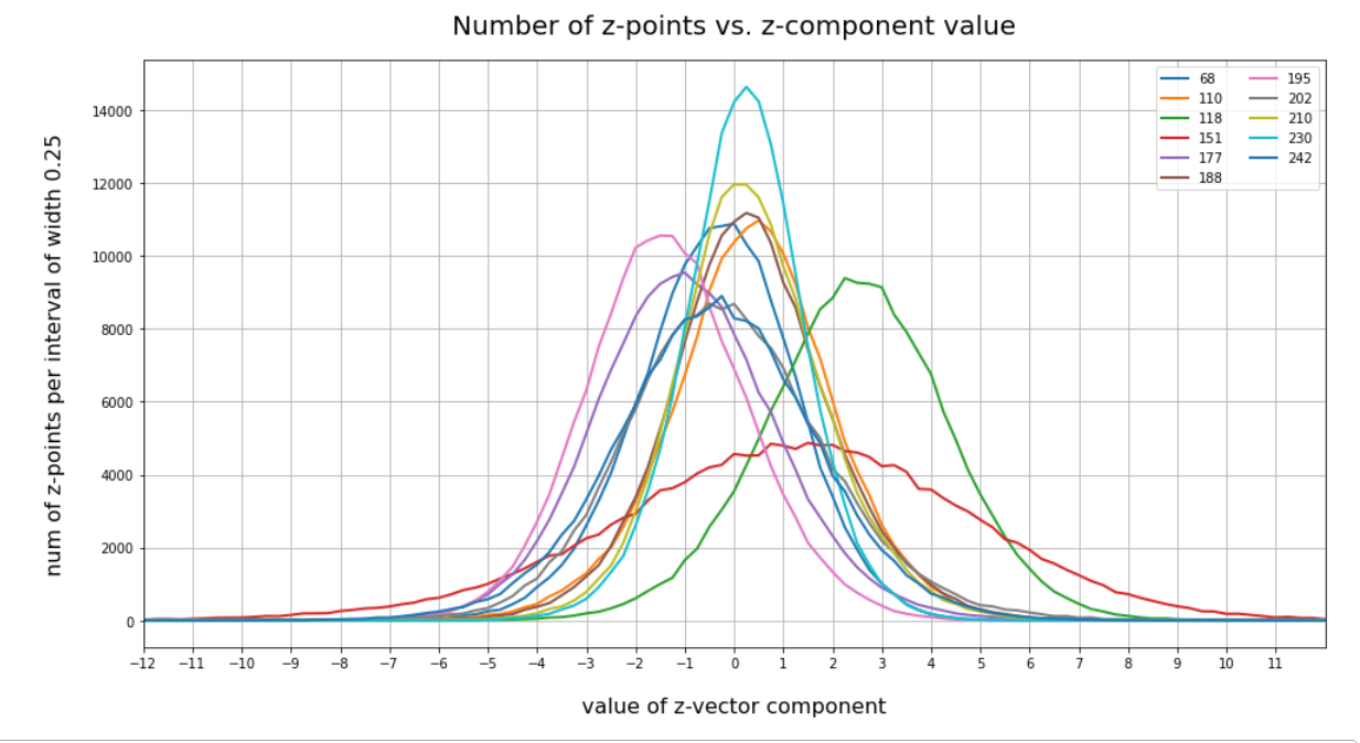
You note, of course, that most of these are components which we already identified as the dominant ones for the orientation and lengths of our latent vectors. Below you see a plot of the number distributions for the values the most important components take:
Visualization of the correlations
It is instructive to look at plots which directly visualize the correlations. Again a code snippet:
import numpy as np
num_per_row = 4
num_rows    = 4
num_examples = num_per_row * num_rows

li_centerx = []
li_centery = []
li_centerx.append(0.0)
li_centery.append(0.0)

#num of plots
n_plots = len(li_ij)
print("n_plots = ", n_plots)

plt.rcParams['figure.dpi'] = 96
fig = plt.figure(figsize=(16, 16))
fig.subplots_adjust(hspace=0.2, wspace=0.2)

#special CelebA point
n_spec_pt = 90415

# statisitcal vectors for b=4.0
delta = 4.0
num_stat = 10
ay_delta_stat = np.random.uniform(-delta, delta, size = (num_stat,z_dim))

print("shape of ay_sel_pts : ", ay_sel_pts.shape)

n_pair = 0
for j in range(num_rows):
    if n_pair == n_plots:
        break
    offset = num_per_row * j
    # move through a row
    for i in range(num_per_row):
        if n_pair == n_plots:
            break
        j_c1 = li_ij[n_pair][0]
        j_c2 = li_ij[n_pair][1]
        li_c1 = []
        li_c2 = []
        for npl in range(0, num_pts):
            #li_c1.append( z_points[npl][j_c1] )
            #li_c2.append( z_points[npl][j_c2] )
            li_c1.append( ay_sel_pts[j_c1][npl] )
            li_c2.append( ay_sel_pts[j_c2][npl] )

        # special CelebA point
        li_spec_pt_c1=[]
        li_spec_pt_c2=[]
        li_spec_pt_c1.append( z_points[n_spec_pt][j_c1] )
        li_spec_pt_c2.append( z_points[n_spec_pt][j_c2] )

        # statistical vectors
        li_stat_pt_c1=[]
        li_stat_pt_c2=[]
        for n_stat in range(0, num_stat):
            li_stat_pt_c1.append( ay_delta_stat[n_stat][j_c1] )
            li_stat_pt_c2.append( ay_delta_stat[n_stat][j_c2] )

        # plot
        sp_names = [str(j_c1)+' - '+str(j_c2)]
        axc = fig.add_subplot(num_rows, num_per_row, offset + i +1)
        #axc.axis('off')
        axc.scatter(li_c1, li_c2, s=0.8 )
        axc.scatter(li_stat_pt_c1, li_stat_pt_c2, s=20, color="red", alpha=0.9 )
        axc.scatter(li_spec_pt_c1, li_spec_pt_c2, s=80, color="black" )
        axc.scatter(li_spec_pt_c1, li_spec_pt_c2, s=50, color="orange" )
        axc.scatter(li_centerx, li_centery, s=100, color="black" )
        axc.scatter(li_centerx, li_centery, s=60, color="yellow" )
        axc.legend(labels=sp_names, handletextpad=0.1)
        n_pair += 1
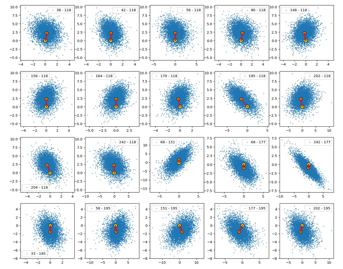
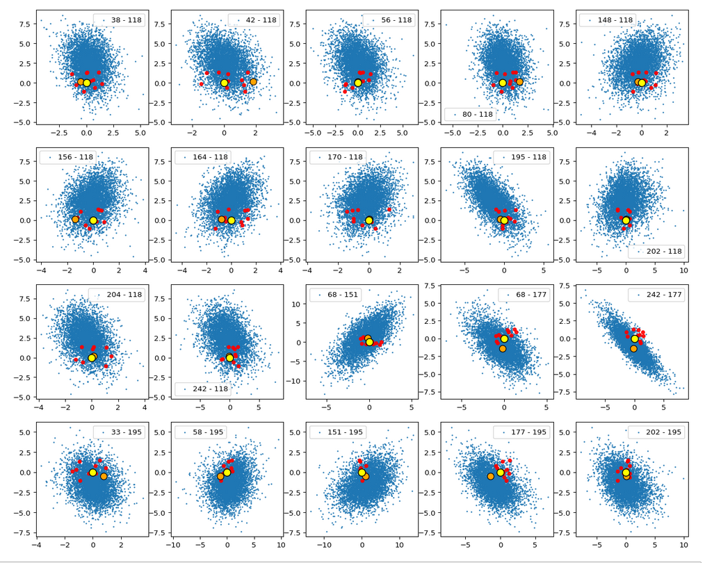
The result is:
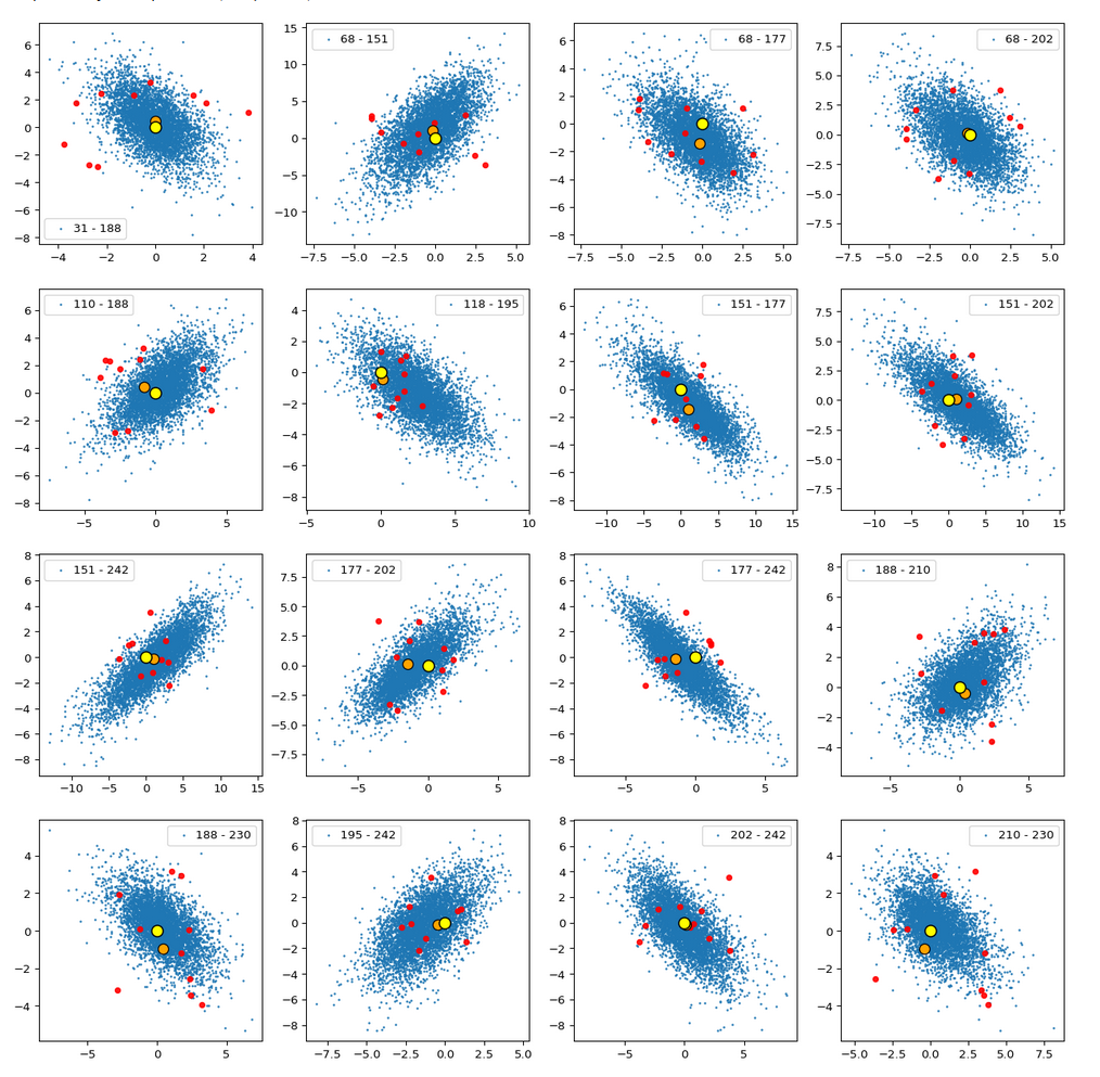
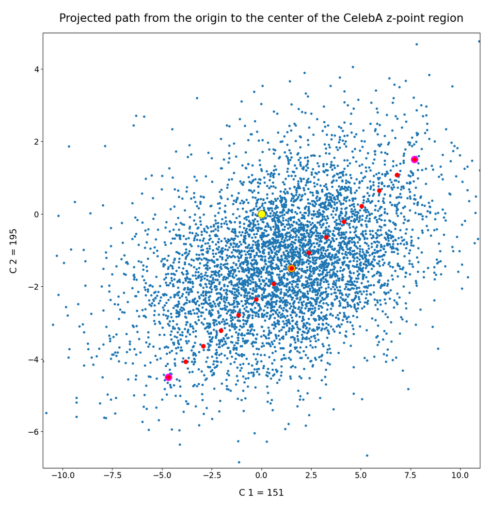
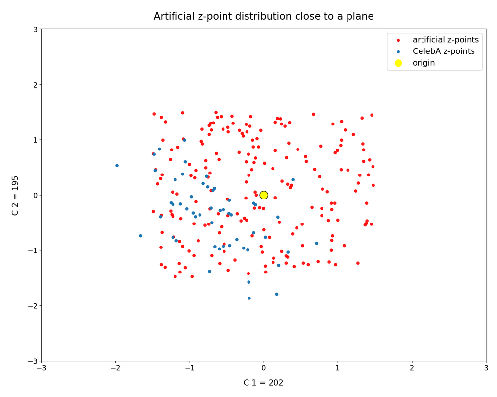
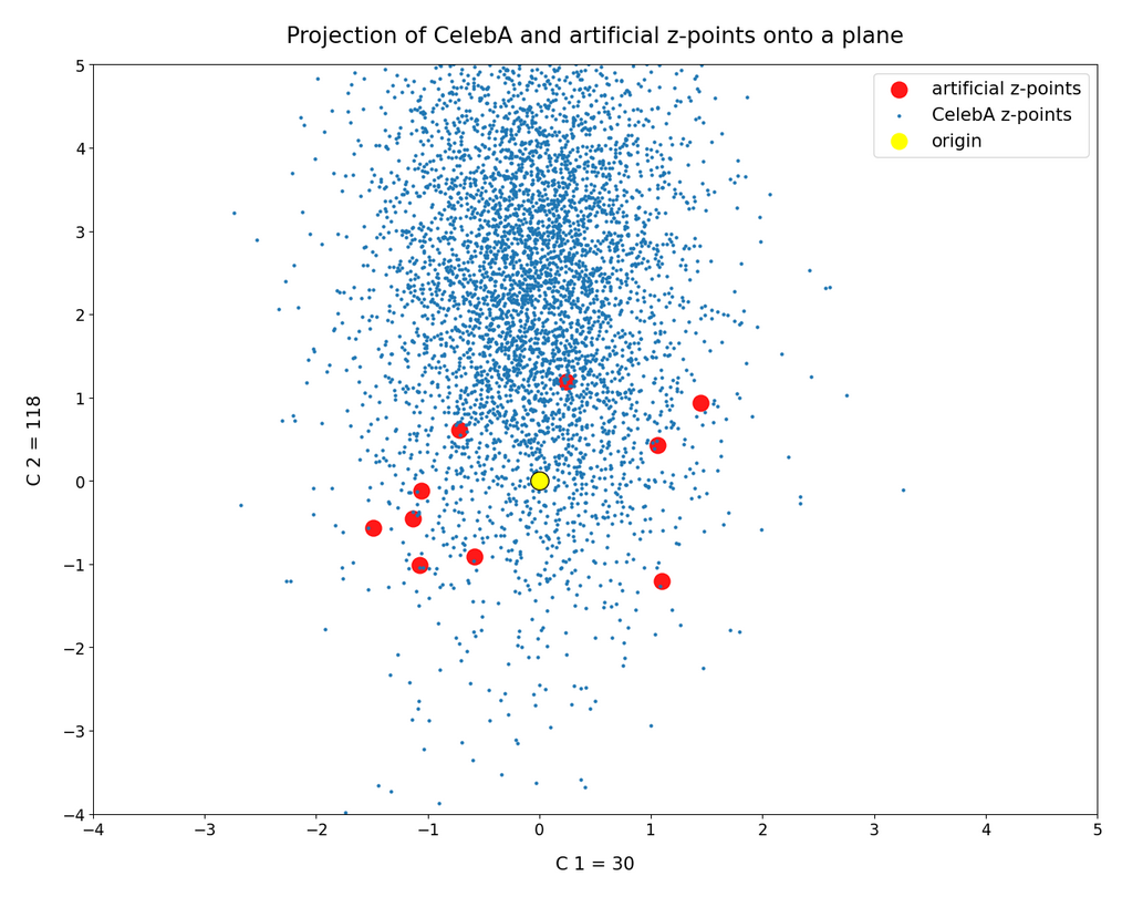
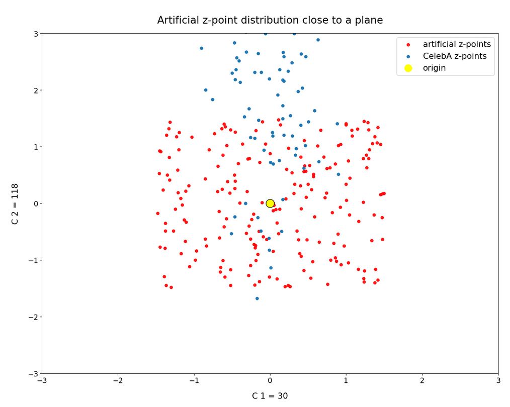
The (5000) blue dots show the component values of the randomly selected latent vectors for CelebA images. The yellow dot marks the origin of the latent space’s coordinate system. The red dots correspond to artificially created random vectors for b=4.0. The orange dot marks the values for one selected CelebA image. We also find indications of an ellipsoidal form of the z-point region for the CelebA dataset. But keep in mind that we only a re looking at projections onto planes. Also watch the different scales along the two axes!
Interpretation
The plots clearly show some average correlation for the depicted latent vector components (and their related z-points). We also see that many of the artificially created vector components seem to lie within the blue cloud. This appears a bit strange as we had found in the last post that the radii of such vectors do not fit the CelebA vector distribution. But you have to remember that we only look at projections of the real z-points down to some selected 2D-planes within of the multi-dimensional space. The location in particular projections does not tell you anything about the radius. In a later sections I also show you plots where the red dots quite often fall outside the blue regions of other components.
I want to draw your attention to the fact that the origin seems to be located close to the border of the region marked by some components. At least in the present projection of the z-points to the 2D-planes. If we only had the plots above then the origin could also have a position outside the bulk of CelebA z-points. The plots confirm however what we said in the last post: The CelebA vector distributions has its center off the origin.
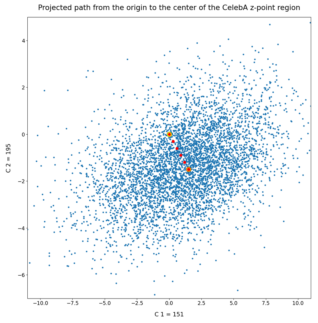
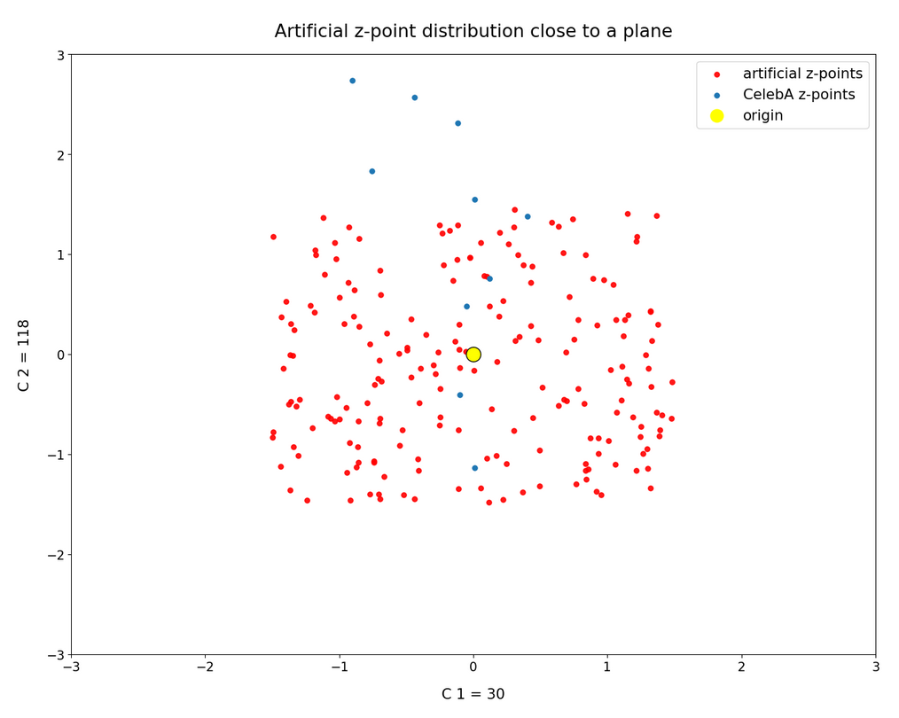
We also see an indication that the density of the z-points drops sharply towards most of the border regions. In the projections this becomes not so clear due to the amount of points. See the plot below for only 500 randomly selected CelebA vectors and the plots in other sections below.
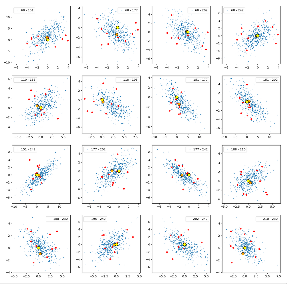
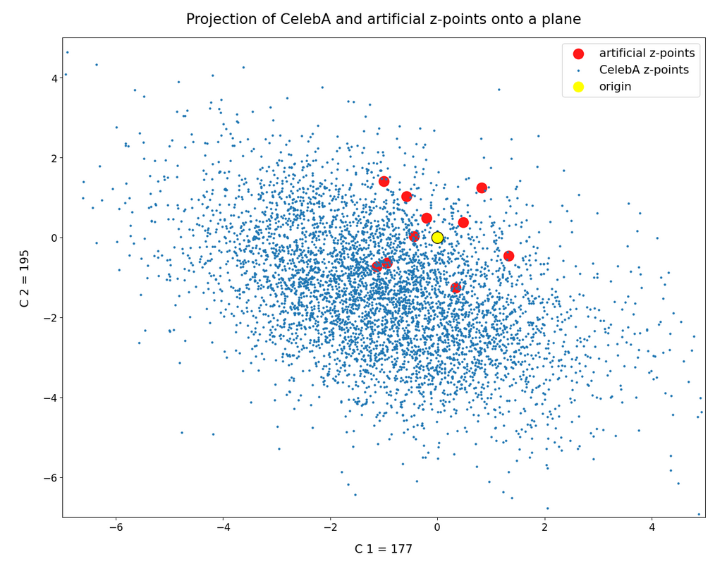
Border position of the origin with respect to the latent vector distribution for CelebA
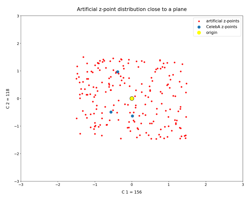
Below you find a plot for 1000 randomly selected CelebA vectors, some special components and b=4.0. The components which I selected in this case are NOT the ones with the strongest correlations.
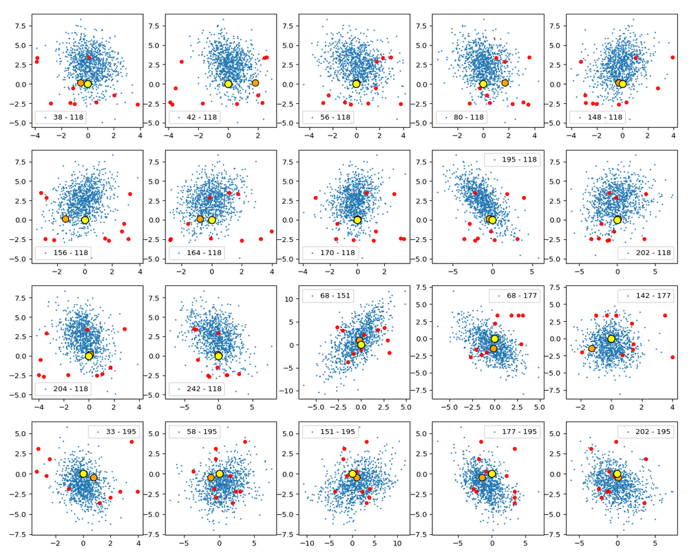
These plots again indicate that the border position of the latent space’s origin is located in a border region of the CelebA z-points. But as mentioned above: We have to be careful regarding projection effects. But we also have the plot of all number distributions for the component values; see the last post for this. And there we saw that all the curves cover a range of values which includes the value 0.0. Together we the plots above this is actually conclusive: The origin is located in a border region of the latent z-point volume resulting from CelebA images after the training of our Autoencoder.
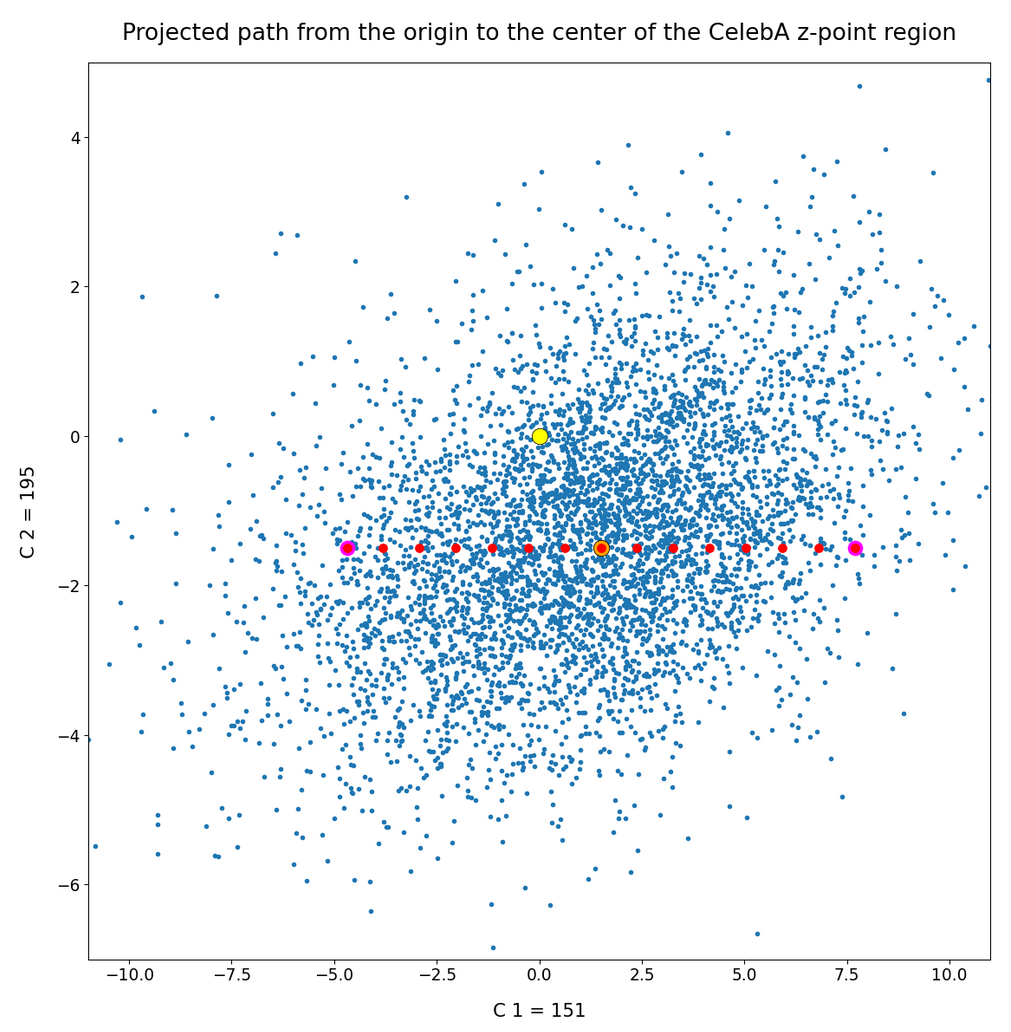
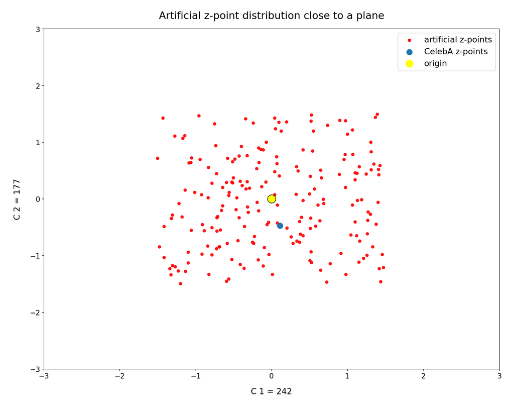
This fact also makes artificial vector distributions with a narrow spread around the origin determined by a b ≤ 2.0 a bit special. The reason is that in certain directions the component value may force the generated artificial z-point outside the border of the CelebA distribution. The range between 1.0 < b < 2.0 had been found to be optimal for our special statistical distribution. The next plot shows red dots for b=1.5.
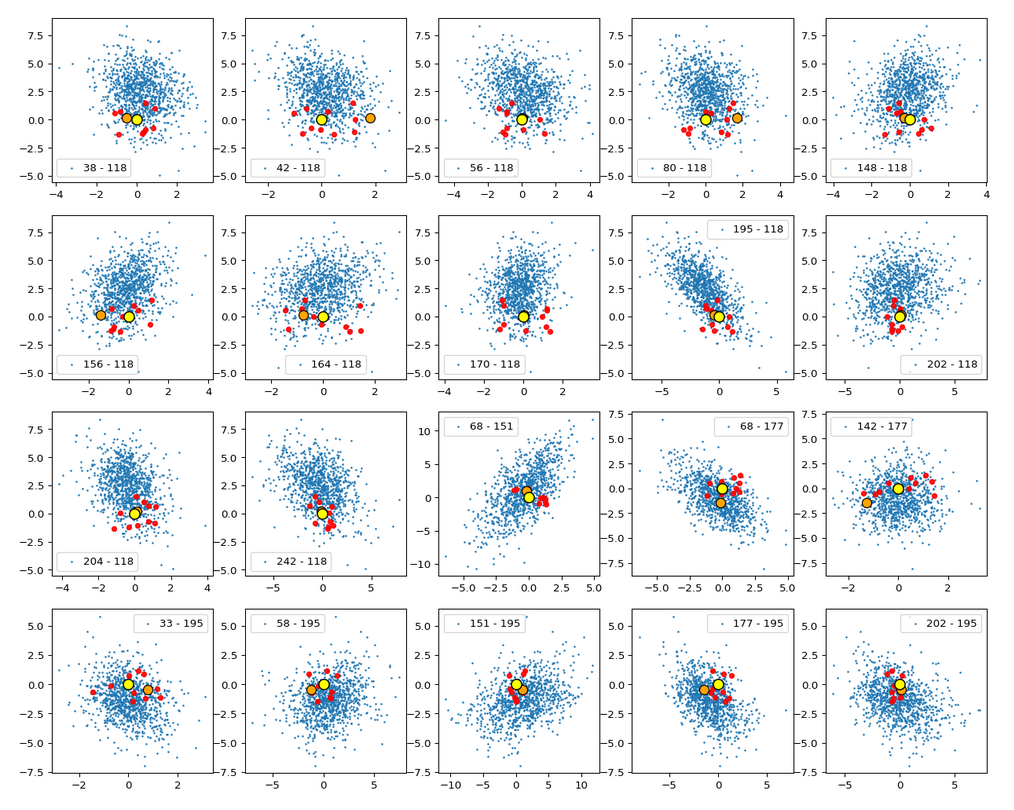
This does not look too bad for the selected components. So we may still hope that our statistical vectors may lead to reconstructed images by the Decoder which show human faces. But note: The plots are only projections and already one larger component-value can be enough to put the z-point into a very thinly populated region outside the main volume fo CelebA z-points.
Conclusion
The values for some of the components of the latent vectors which a trained convolutional AE’s Encoder creates for CelebA images are correlated. This is reflected in plots that show an orthogonal projection of the multi-dimensional z-point distribution onto planes spanned by two coordinate axes. Some other components also revealed that the origin of the latent space has a position close to a border region of the distribution. A lot of artificially created z-points, which we based on a special statistical vector distribution with constant probabilities for each of the independent component values, may therefore be located outside the main z-point distribution for CelebA. This might even be true for an optimal parameter b=1.5, which we found in our analysis in the last post.
We will have a closer look at the border topic in the next post:
Autoencoders and latent space fragmentation – IV – CelebA and statistical vector distributions in the surroundings of the latent space origin