My present post series explores options to use a standard convolutional Autoencoder [AE] for the creation of images with human faces. The face generation should based on random input to the AE’s Decoder. On our quest for a suitable method we have meanwhile learned a lot about other aspects of Autoencoders, vector distributions in multi-dimensional latent spaces and generative methods for our special case:
- Methods to create statistical latent vectors [z-vectors] as input for the AE’s Decoder must be chosen carefully. Among other things: It is difficult to create a bunch of random vectors which cover wider areas in the vastness of a multidimensional space. So the z-vector creation must be adjusted to specific requirements.
- After having been trained with CelebA images a convolutional AE fills a limited and coherent region in the latent space with z-points for the training images. This latent space region appears to be critical for successful image creation: Statistically generated z-vectors should point to this region. The core of the z-point distribution gets filled relatively densely.
- A convolutional AE maps human face images onto an approximate multivariate normal distribution. This gives the inner core of the z-point distribution the structure of a multidimensional ellipsoid. The projections of this ellipsoid onto 2-dimensional coordinate planes show characteristic nested elliptic contour lines.
- As the main axes of these ellipses were inclined with different angle towards the axes of chosen coordinate planes we concluded that linear correlations mark average dependencies between the z-vector components. Limiting conditions imposed by these correlations must also be fulfilled by z-vectors used as the Decoder’s input.
See previous posts in this series for more details. In particular, the last 2 posts
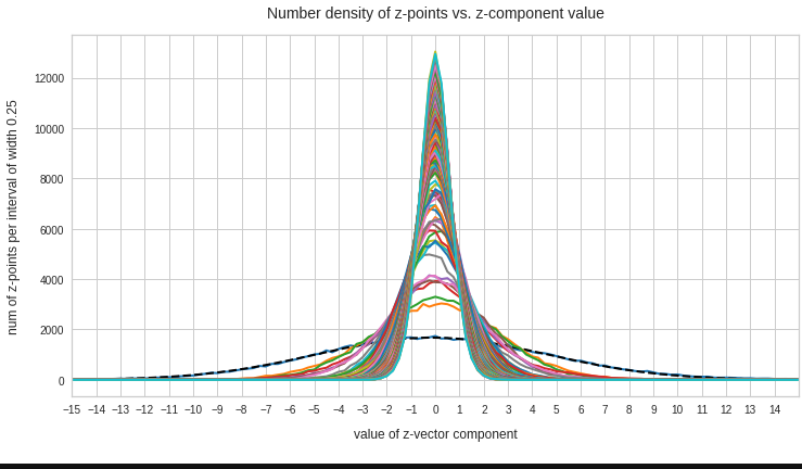
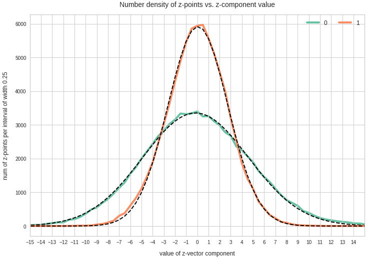
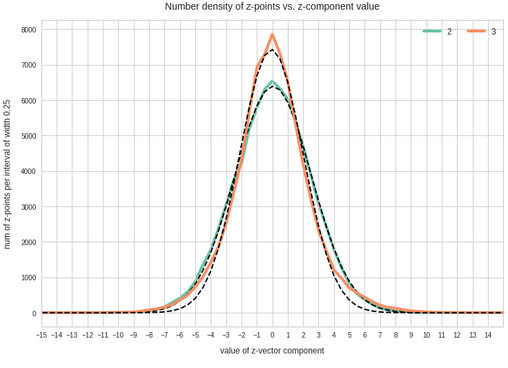
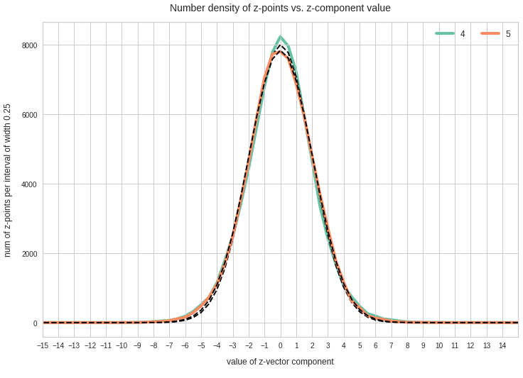
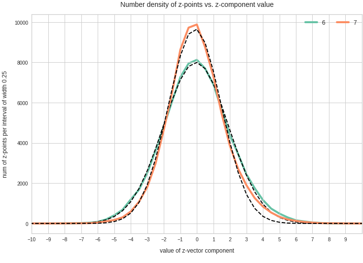
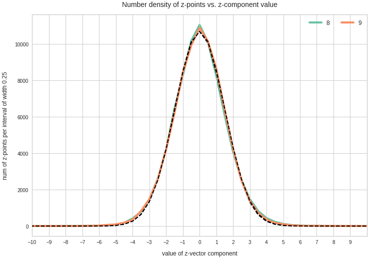
have shown that the density distribution for the z-points really exhibits elliptic contour lines in the original coordinate system of the latent space and (!) in the target coordinate system of a PCA transformation.
In this post we use our gathered knowledge: I present a first simple method to generate z-vectors which point to the latent space region filled by z-points for CelebA images. These z-vectors will fulfill the general and limiting elliptic conditions for their components.
Decomposing the full problem of latent vector generation into a sequence of 2-dimensional problems
The nice thing about multivariate Gaussian distributions with linear correlations between the vector components is the following: We can reduce the problem of choosing proper component values to a series of 2-dimensional restrictions. Firstly we can use characteristic properties of the Gaussian distribution for each component. And secondly we can use confidence ellipses in 2-dimensional coordinate planes to restrict the component values to allowed intervals.
Ellipses are most easy to handle when their axes are aligned with the axes of the coordinate system in which we describe them. So, let us assume that we know an affine transformation T to a new coordinate system which also has orthogonal axes and supports the following special transformation properties for a multivariate normal density distribution:
- T maps nested elliptic contour lines of the multidimensional density distribution and in particular confidence ellipses for component pairs in the original coordinate system to nested elliptic contours and confidence ellipses in the new coordinate system.
- Taligns the centers of the transformed ellipses with the origin of the new coordinate system.
- T aligns the main axes of the mapped ellipses with the axes of the new coordinate system.
- T is reversible.
How could we then use the transformed data for vector-creation?
In the new coordinate system, a contour ellipse in a chosen coordinate plane for the axes-indices (i, j) may have main diameters of size
d1 = 2 * a and d2 = 2 * b.
We then can first select a random v_i value to fall into a range [-a * fact, a * fact].
– fact * a < v_i < fact * a
With fact being a proper factor. This factor defines a confidence level in the new coordinate system. With the value of v_i fixed and b being the half-diameter in the orthogonal direction the correlation condition for the z-point distribution says that the v_j value must fall into an interval [-c, c] defined by:
-c < v_j < c,
with c = b * fact * sqrt(1 – x**2 / (fact * a)**2)
But within these limits we can again choose the v_j-value freely. Below I use a simple random-function for a constant probability density to pick a value.
However: It would not be enough to restrict the coordinates to the conditions of just one ellipse! The components of the created vectors must in parallel fulfill elliptic conditions for all of the possible pairs of vector-components. I.e. we may need to adapt the v_j values gained from the analysis of a fist 2D-ellipse to further conditions of other ellipses and component pairs. This can be achieved by an iteration. For z_dim = 256 this involves a total of 32640 checks and possible value-adaptions to each and all of the allowed value ranges.
In addition: The order by which the component-pairs and their conditions are investigated must be randomized to get real statistical vector distributions.
Eventually the resulting vector components must be re-transformed into the original coordinate system of the latent space.
The ellipse for the “core’s boundary” in the original coordinate system will be defined by the chosen confidence level of the ellipsoidal normal distribution. We saw already that a confidence level of σ = 2.0 defines the transition to outer regions of the z-point density distribution quite well.
This all sounds manageable by relative simple Python programs. But: Do we know a proper transformation T? Yes, we do: A PCA-transformation of the z-point density distribution has all the properties discussed above.
Using half maximum values after a PCA transformation of the z-point distribution
The last post proved that a PCA transformation maps ellipses onto ellipses for component pairs in the transformed PCA coordinate system. The advantage of the ellipses there is that their main axes are on average well aligned with the orthogonal PCA coordinate axes. Gaussians for the number density distribution per component are mapped to Gaussians for the new components in the transformed coordinate system. So, the basic idea for a proper z-vector generation is:
- Take the multivariate normal z-point distribution for the training images in the AE’s latent space.
- Apply a PCA analysis to diagonalize the correlation matrix and transform the z-vector components to the PCA coordinate system.
- Use the ellipses in coordinate planes of the PCA coordinate system to create random z-vector components fulfilling all required conditions there.
- Re-transform the resulting z-vector components into the original coordinate system of the latent space.
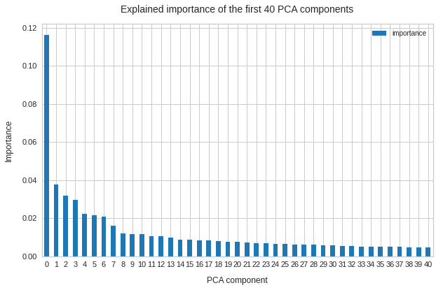
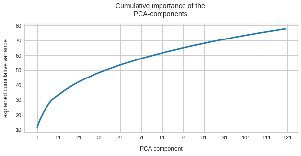
Point 3 in our method is covered by a numerical analysis of the Gaussians in the PCA-coordinate system. We determine the half-width numerically by analyzing the density distribution with the help of sampling intervals. This simple method has resolution limits related to the size of the sampling interval. This has consequences for PCA components with a small standard deviation. We saw already in the last posts that such distributions appear for higher PCA components at the lower end of the explained variance.
Does the suggested method work?
The convolutional AE we work with was defined in previous posts with 4 Conv2D layers in the Encoder and 4 Conv2DTranspose layers in Decoder. The number of latent space dimensions was z_dim = 256. The AE network was trained on CelebA images. I do not want to bore you with details of the codes for the creation of z-vectors consistent to the resulting elliptic conditions. It is all standard. The PCA-transformation can e.g. be taken from the sklearn-package.
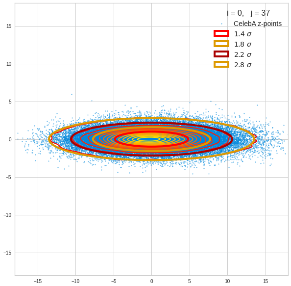
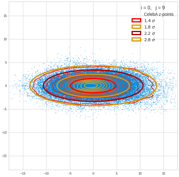
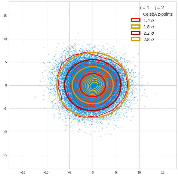
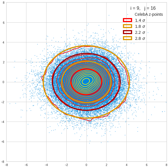
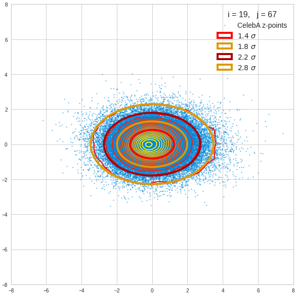
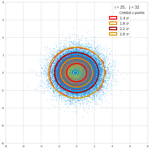
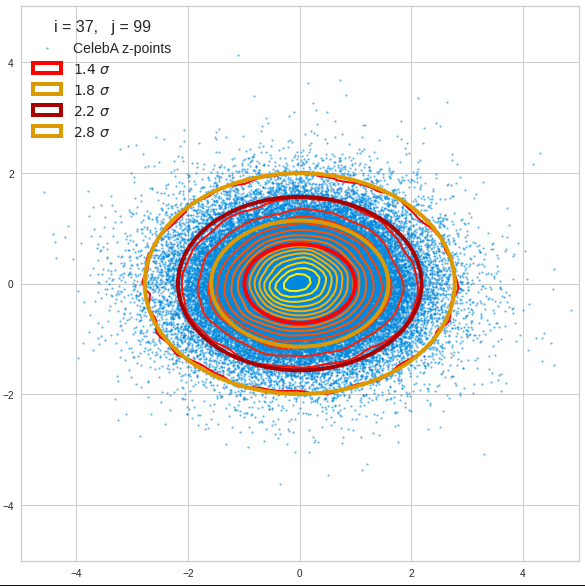
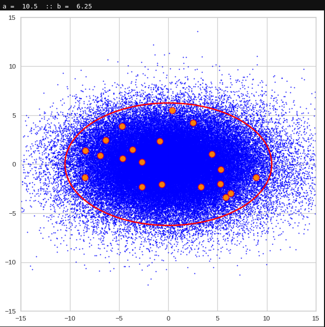
I have applied a constant probability density to choose a random value within the allowed ranges for the component values of the aspired z-vectors in the PCA coordinate system. For the plots below I have used the most important 50 to 105 PCA components (out of 256). The plots include confidence ellipses on a level of σ = 2.2. I derived the confidence ellipses by directly evaluating the standard deviations of the transformed distribution data in all coordinate directions.
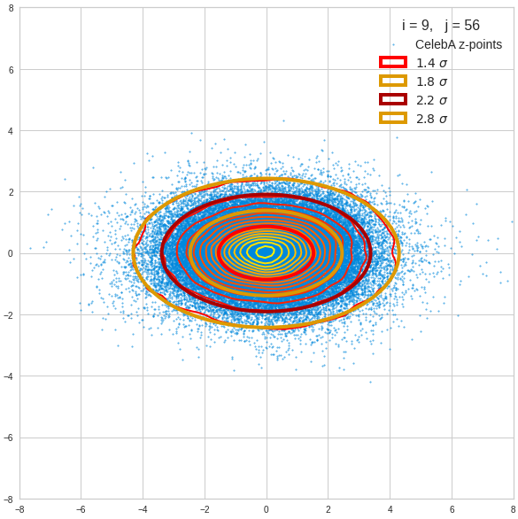
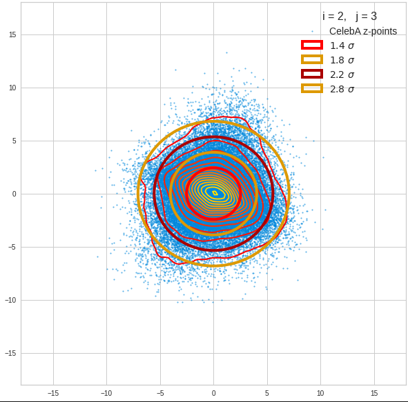
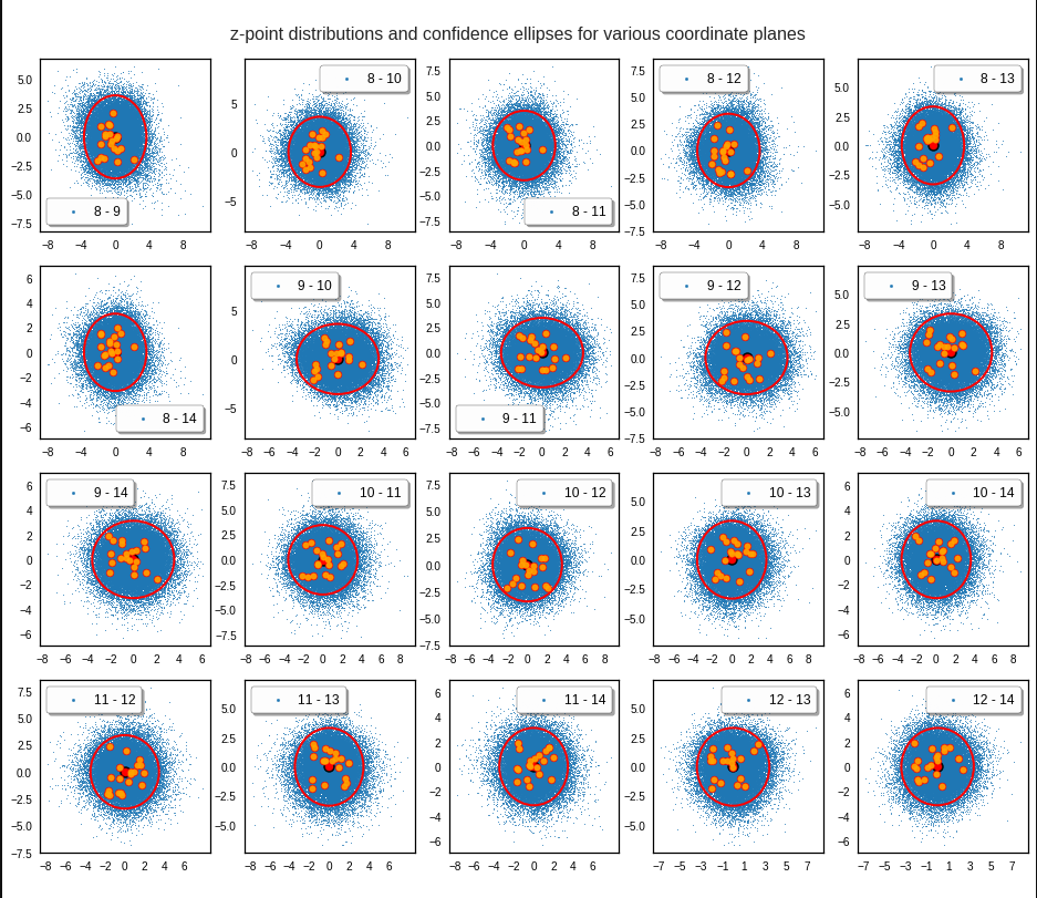
The first plot shows you such an ellipse for the coordinate plane corresponding to the first two, most important PCA components. The orange points mark 20 z-points defined by 20 randomly z-vectors fulfilling all elliptic conditions. The plot contains 120,000 z-points for images out of the 170,000 CelebA pictures used during training.
Generated statistical vectors in the PCA coordinate system
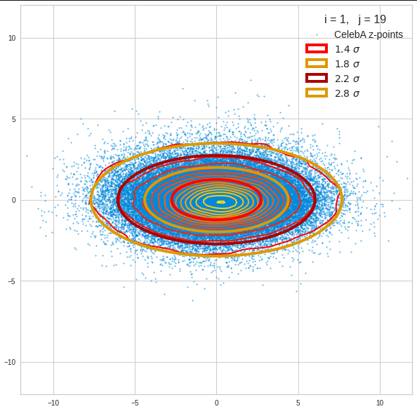
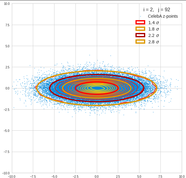
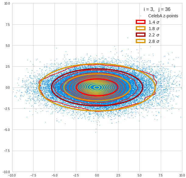
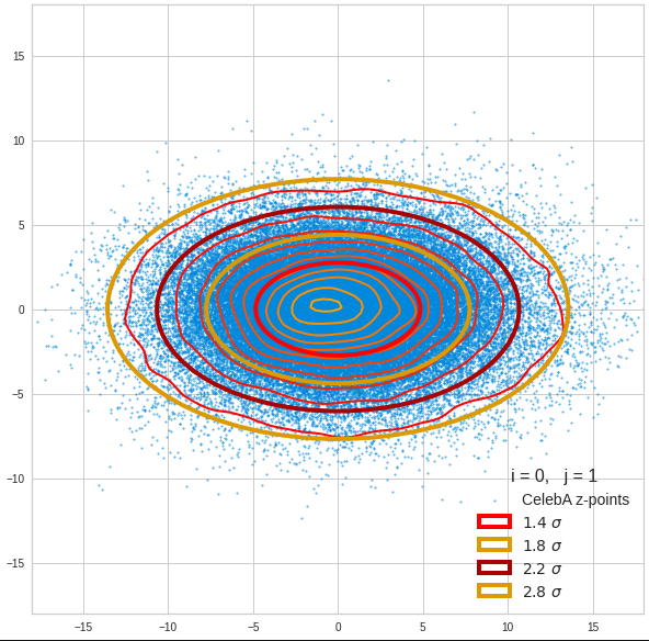
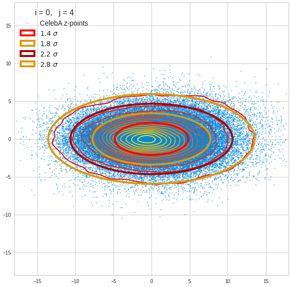
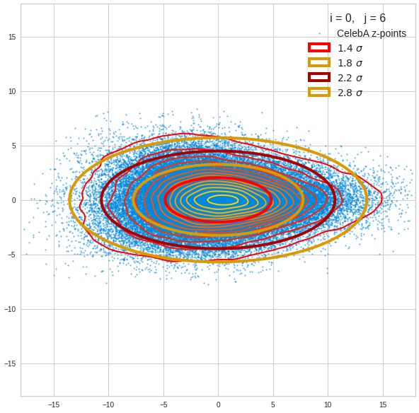
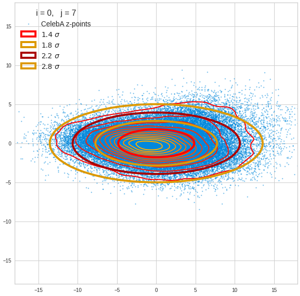
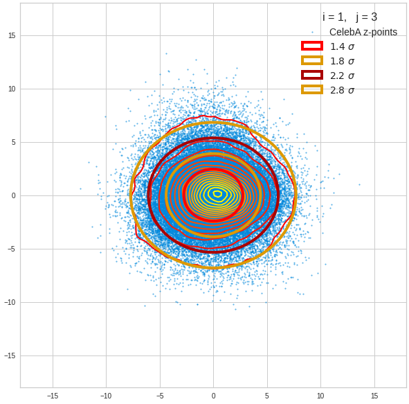
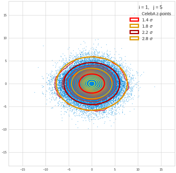
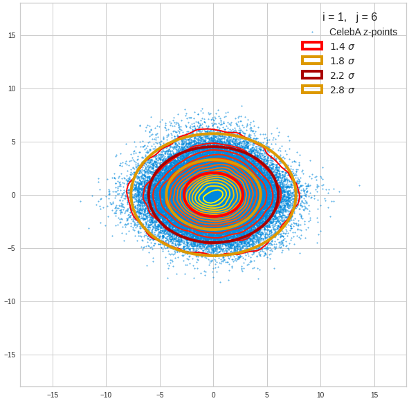
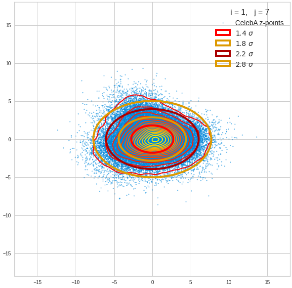
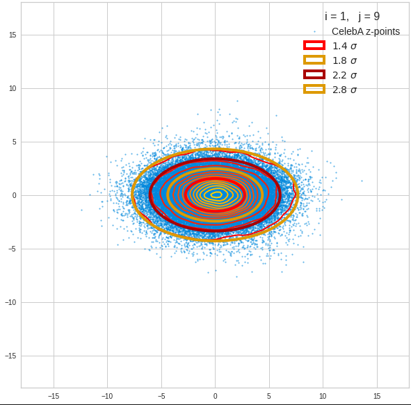
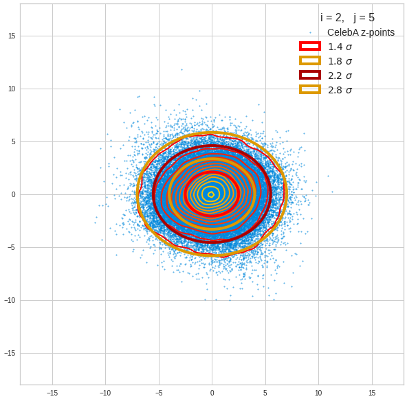
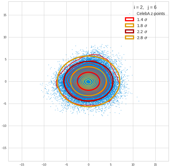
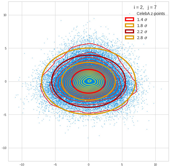
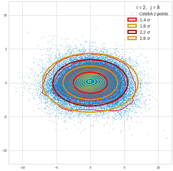
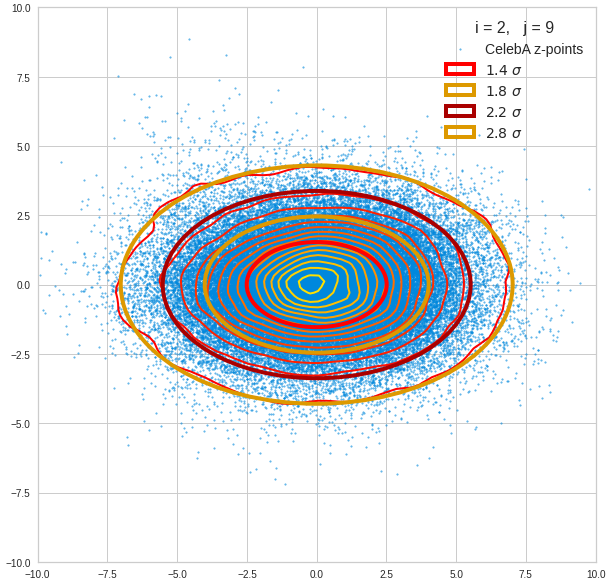
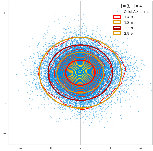
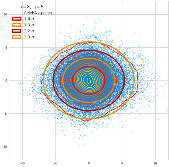
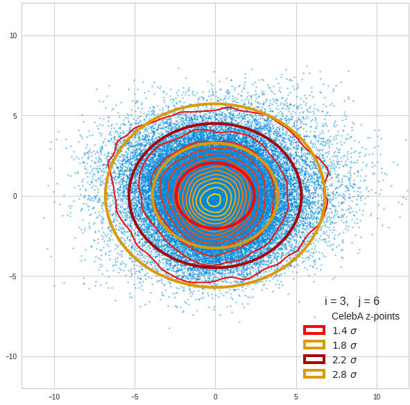
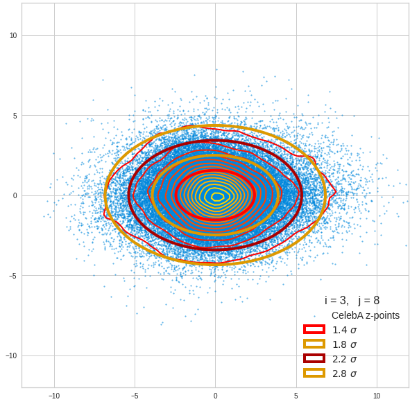
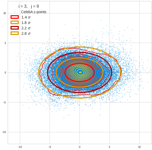
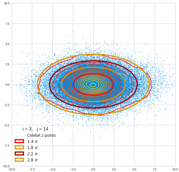
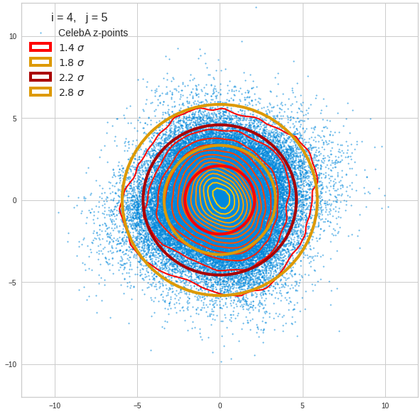
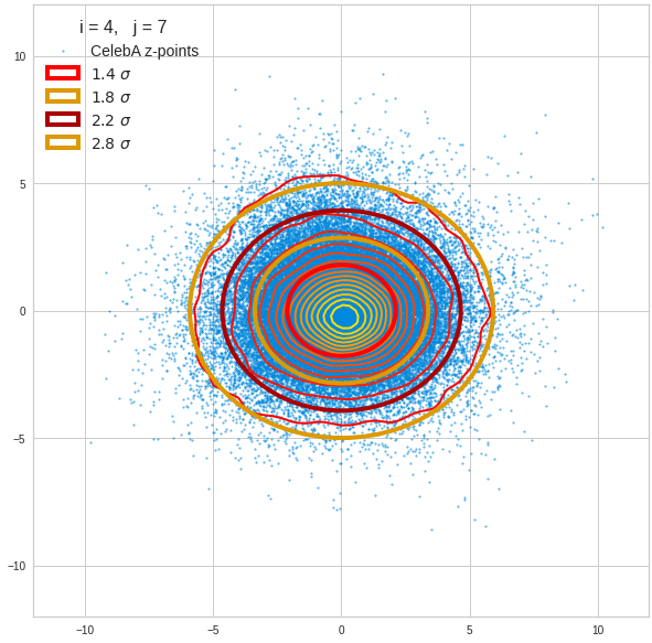
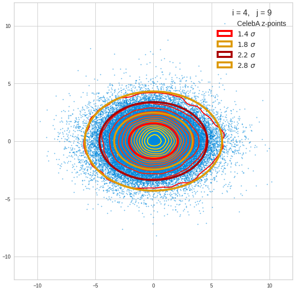
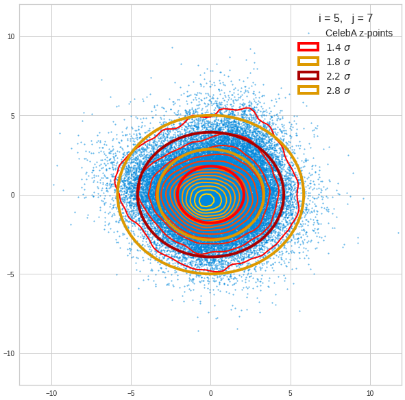
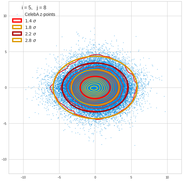
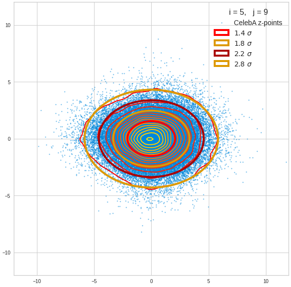
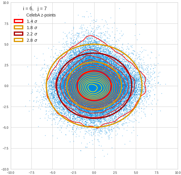
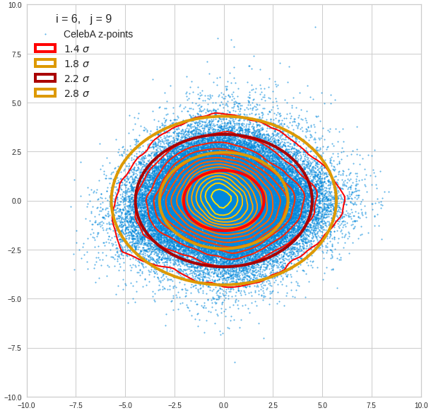
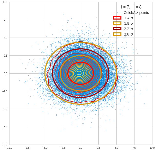
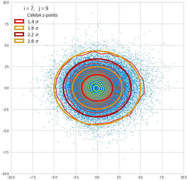
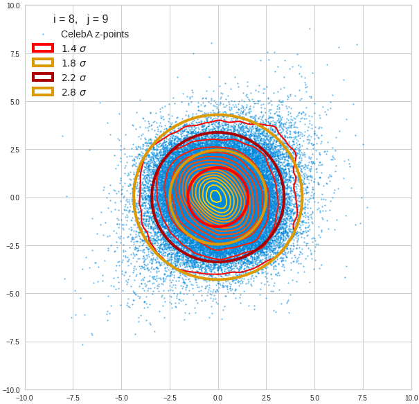
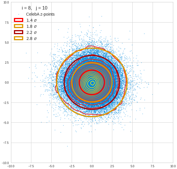
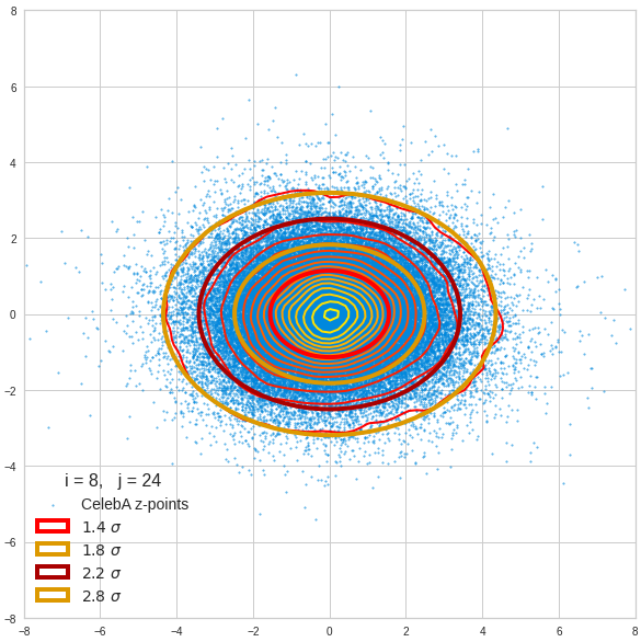
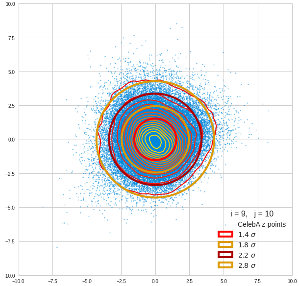
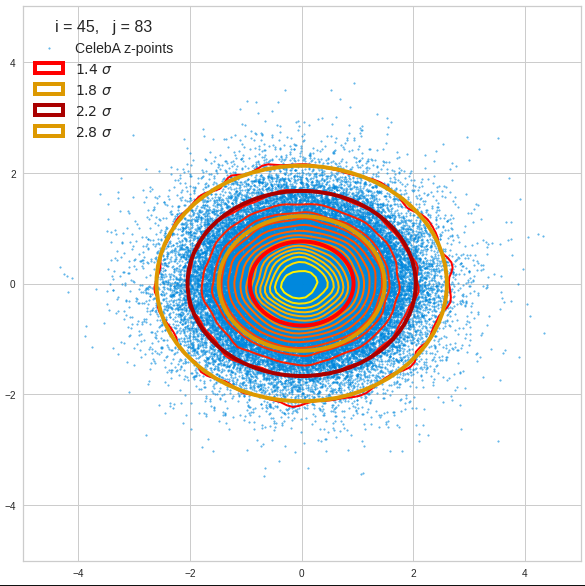
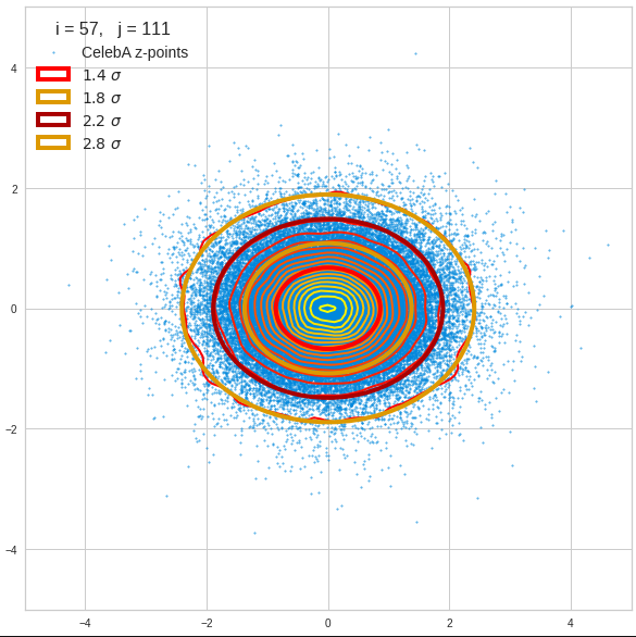
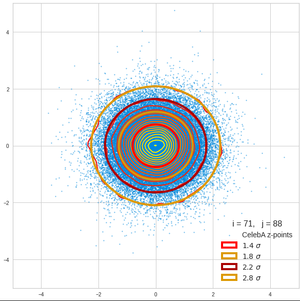
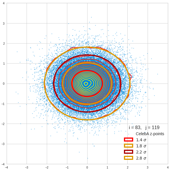
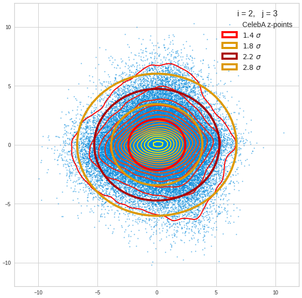
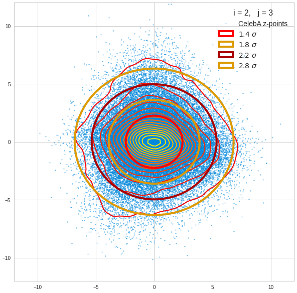
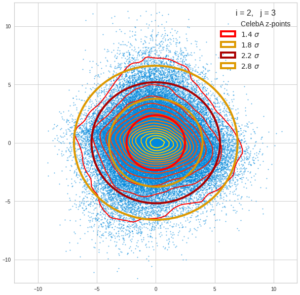
For elliptic contour lines see the last post before the present one in this series. The next plot shows the same generated 20 z-vectors for other component-combinations among the first 20 of the most important PCA-components. The plots contain a selection of 60,000 z-points.
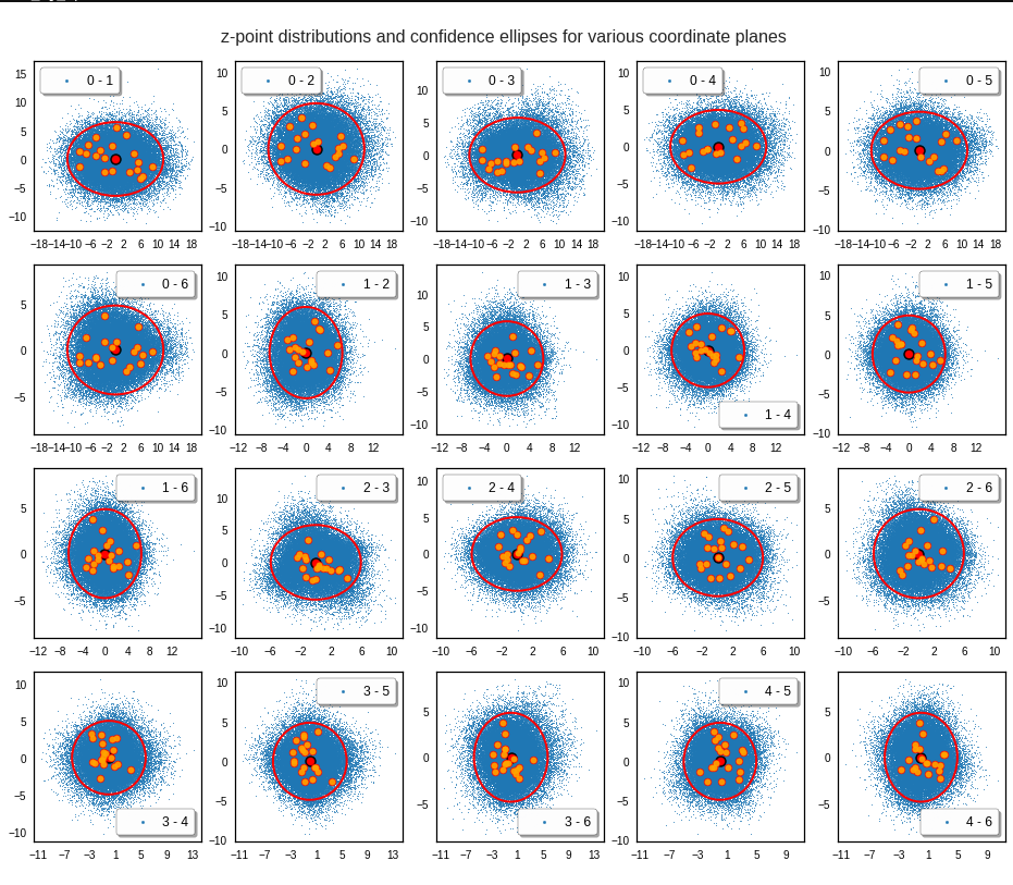
The outer z-points points do not always indicate that we have elliptic contours in the denser core of the displayed 2-dimensional distributions. But see the last post for proofs that the inner core inside the red ellipse really displays elliptic contours. You see that all random vectors lie within the 2-σ-ellipses.
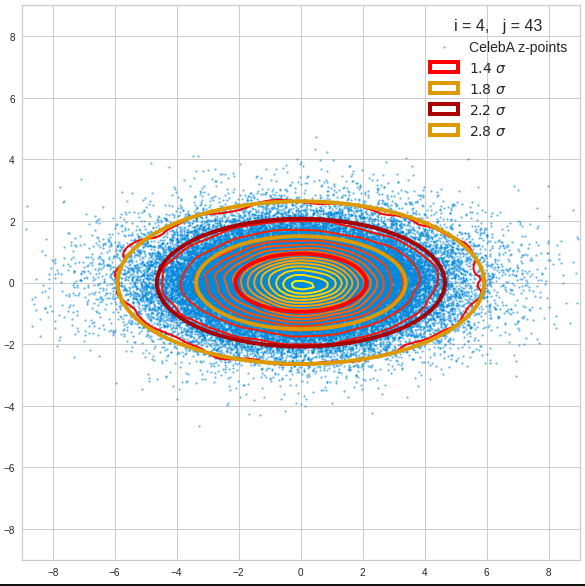
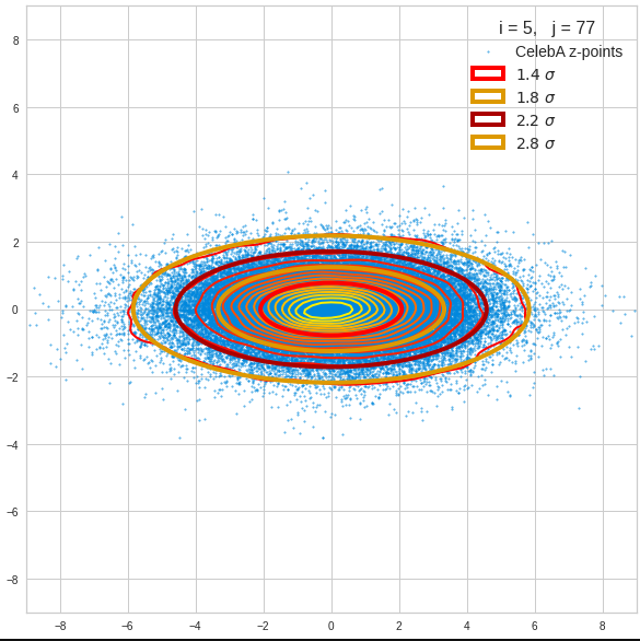
The next plot shows the generated z-vectors in the original coordinate system of the latent space. The component values were back-transformed from the PCA-system to the original coordinate system.
Generated statistical z-vectors after an inverse PCA transformation to the original coordinate system of the latent space
![]()
We get similar plots for other component pairs. And of course for other generated vectors.
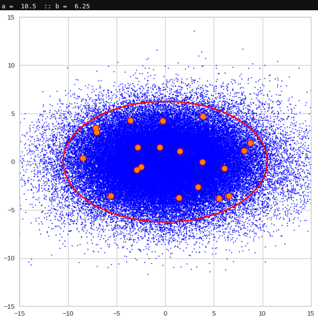
Generated statistical z-vectors in the PCA coordinate system
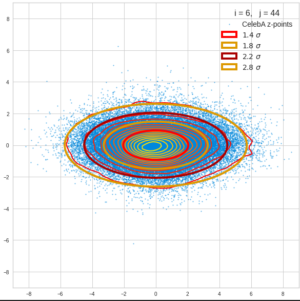
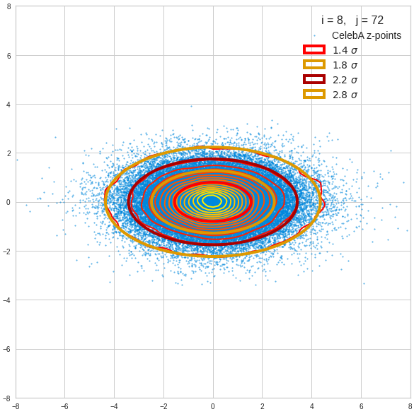
Generated statistical z-vectors after an inverse PCA transformation to the original coordinate system of the latent space
![]()
Technically we have obviously achieved what we wanted: Our generated statistical vectors are distributed within the core of our multidimensional ellipsoid.
Note that this method fortunately works even when we use a limited number of the PCA components, only. This is due to intricate properties of a PCA transformation which guarantee that a back-transformation puts the resulting points close to the original ones even when we omit less important PCA components. I cannot discuss the math-details in this blog. You have to see scientific literature for this. An introduction is e.g. provided by https://arxiv.org/pdf/1404.1100.pdf.
For me this property of the PCA transformation was helpful when I ran into the resolution problem for a proper half-width of the Gaussians. Taking 256 components lead to errors as elliptic conditions for very narrow Gaussians were not properly defined and some of the created vectors left the allowed value ranges.
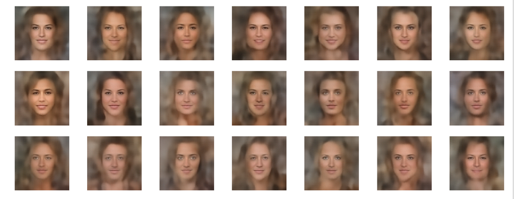
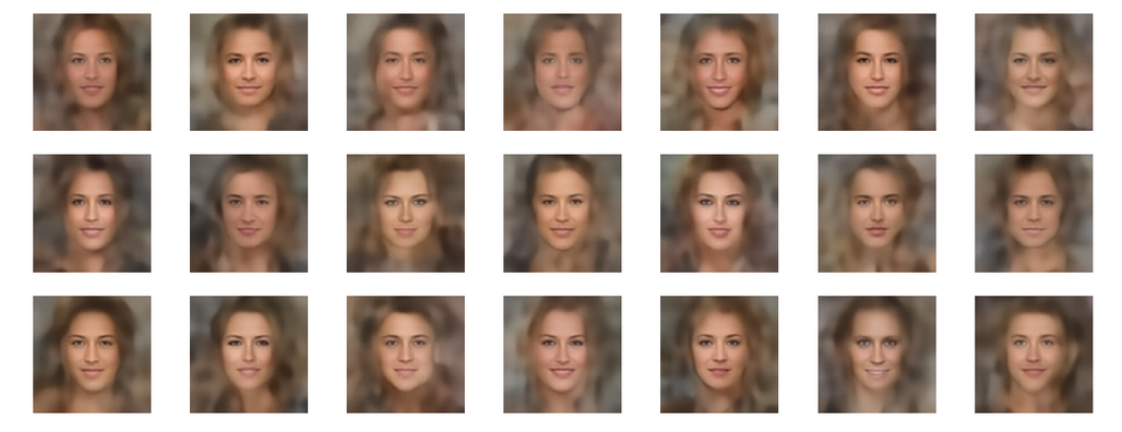
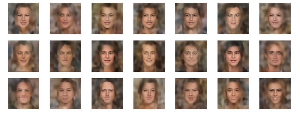
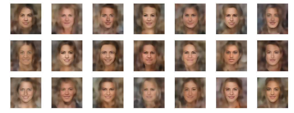
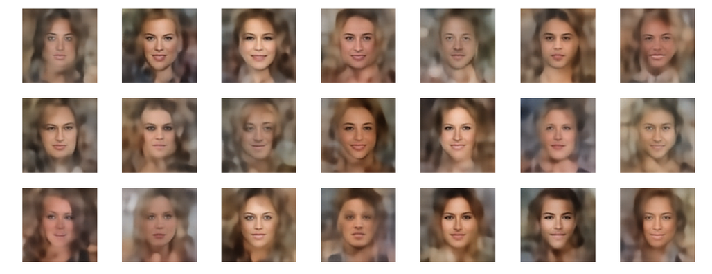
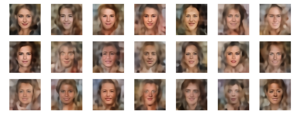
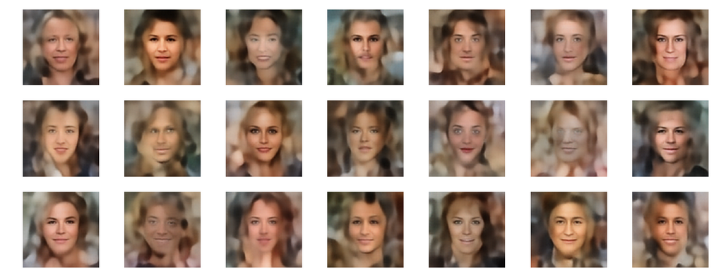
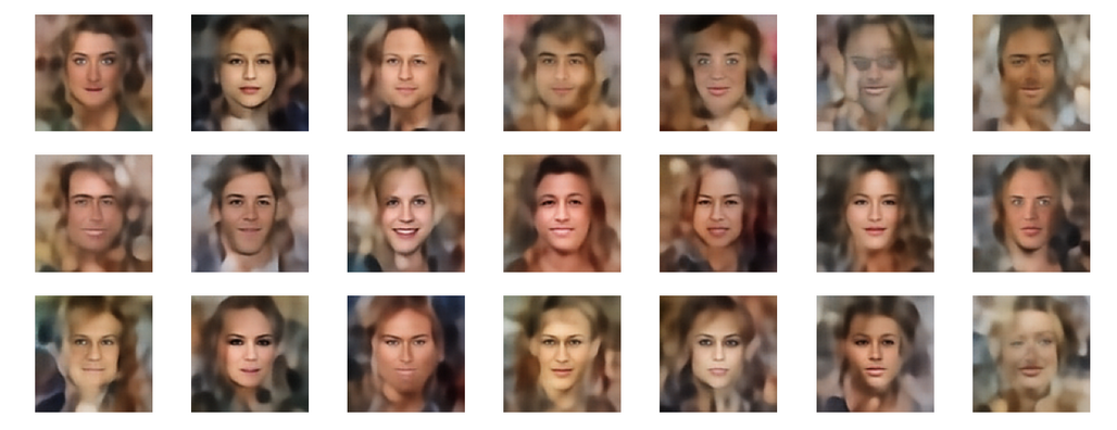
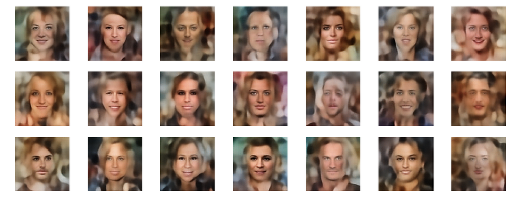
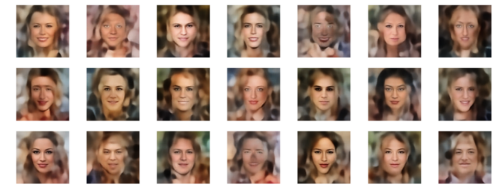
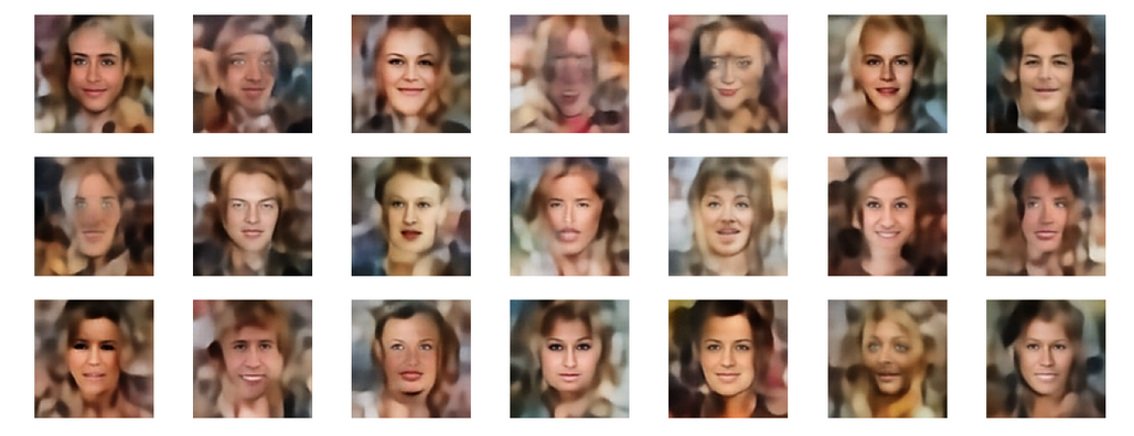
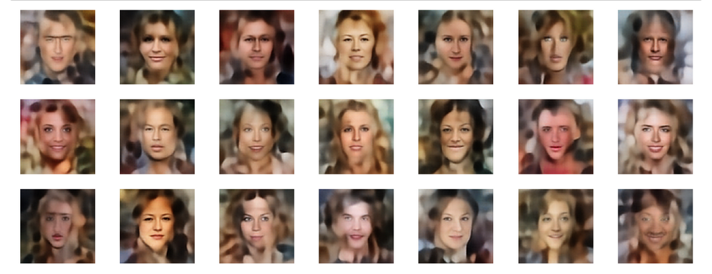
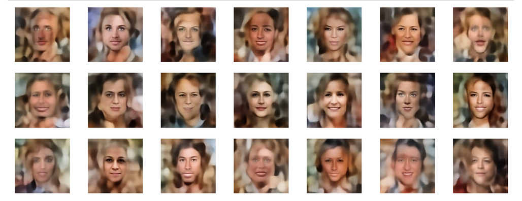
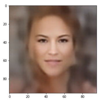
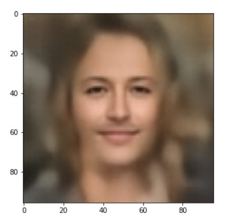
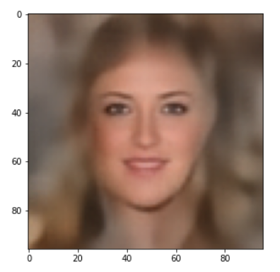
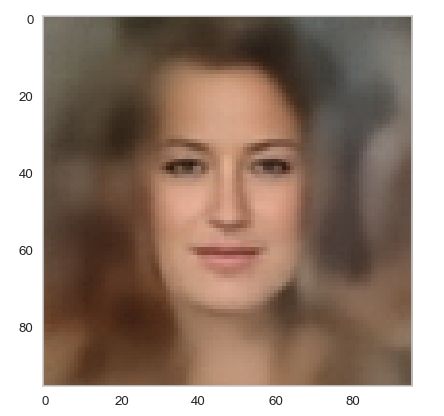
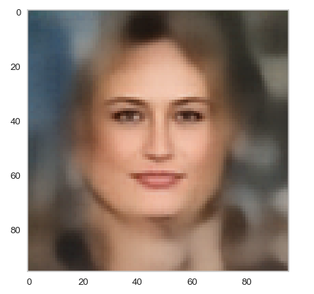
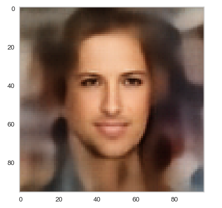
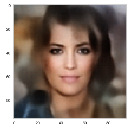
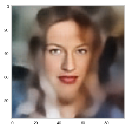
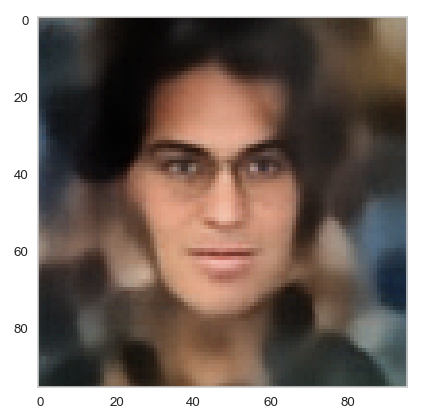
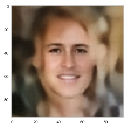
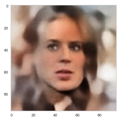
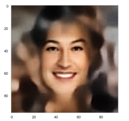
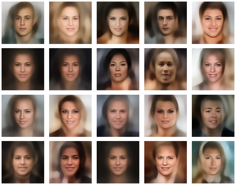
Resulting face images
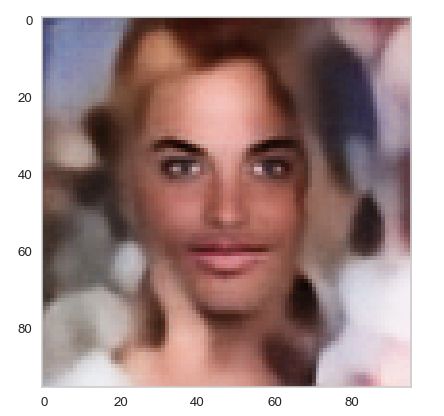
Let us look at some results. First I want to remind you from where we started:
Failed trials with improper random z-vectors based on constant probability densities
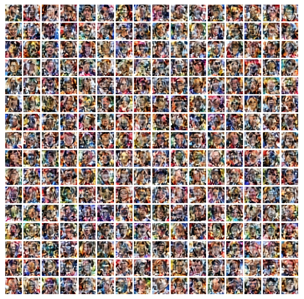
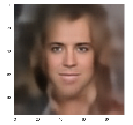
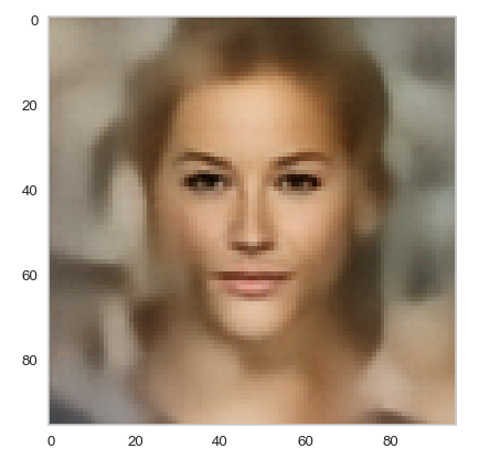
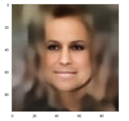
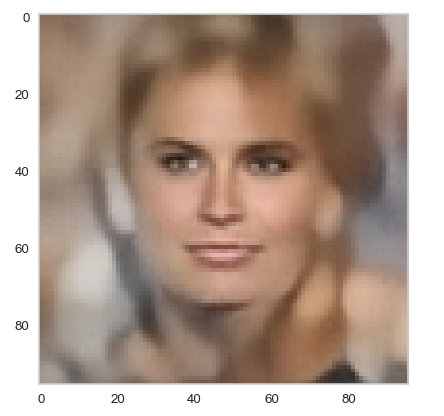
A simple random generator used in the beginning was totally inapt to feed the AE’s Decoder with proper statistical z-vectors. And now – look at the following plots. They were produced for a varying number of PCA components between 50 and 120, 100000 statistically selected z-points within a 3 σ-level for the PCA-transformation and various factors 0.6 < fact < 0.8 used upon a half-width corresponding to a confidence level of 2.35 σ:
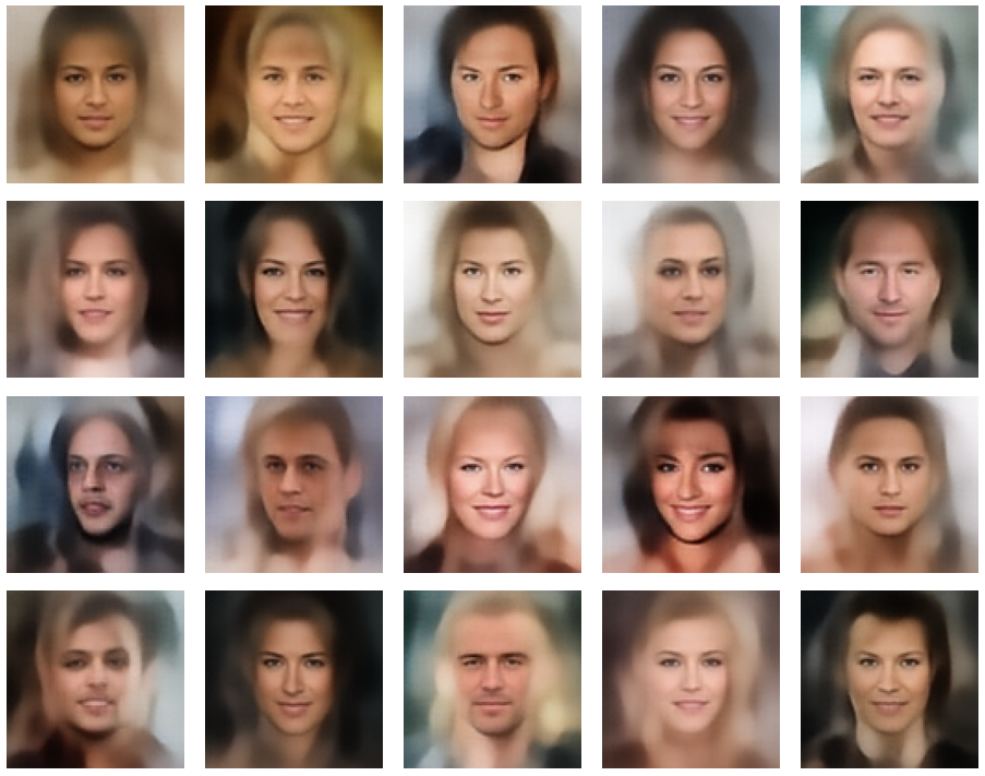
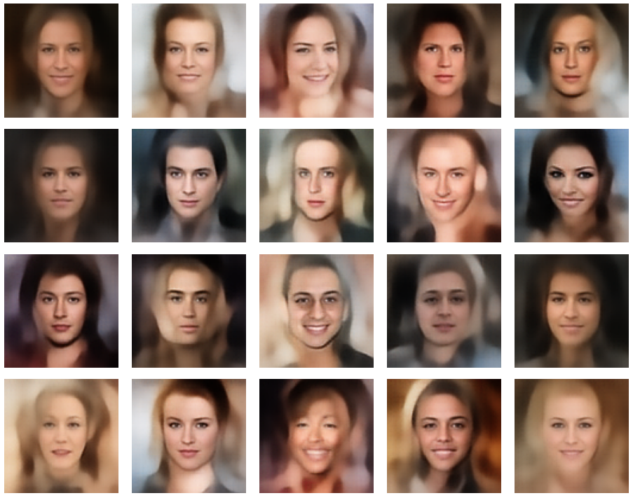
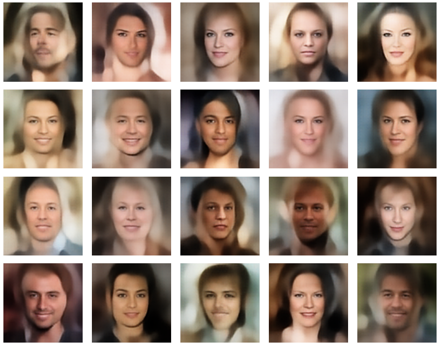
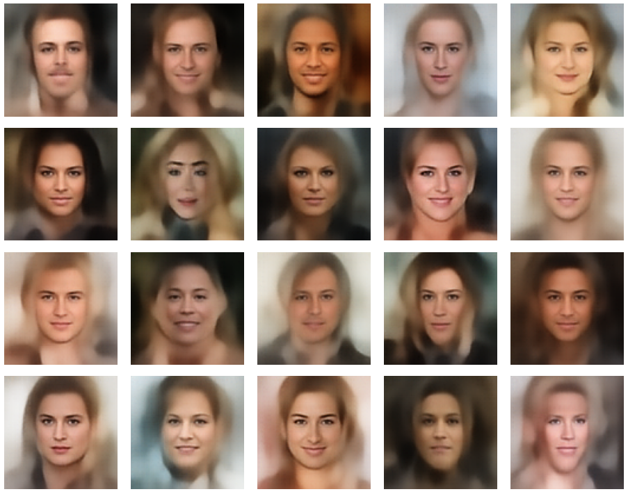
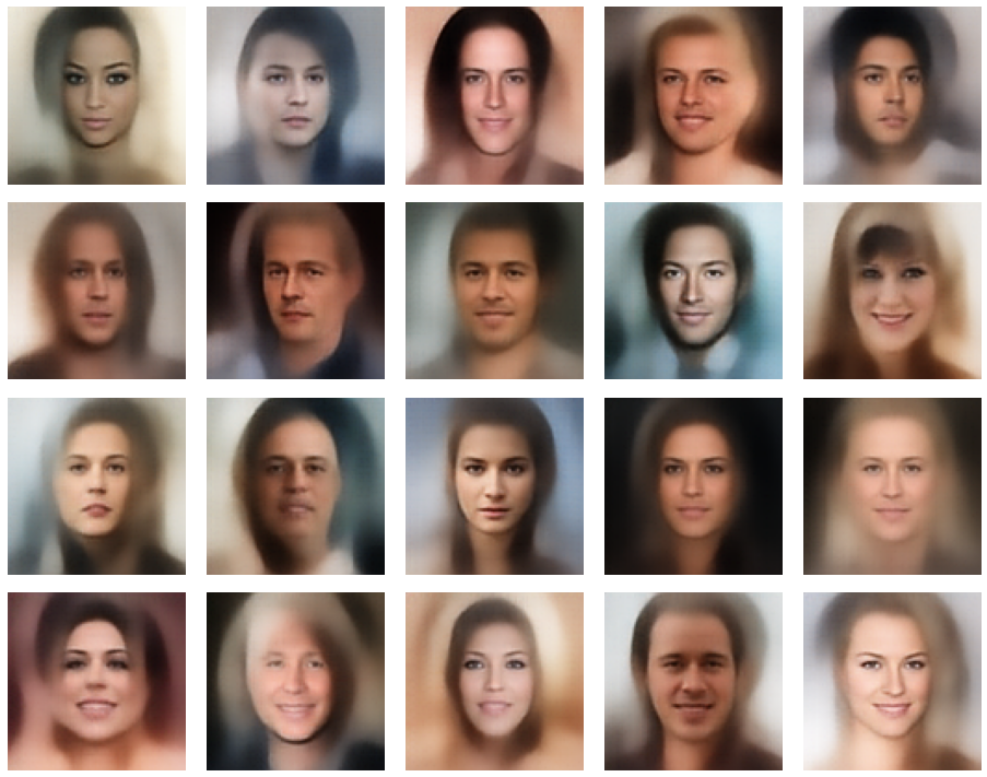
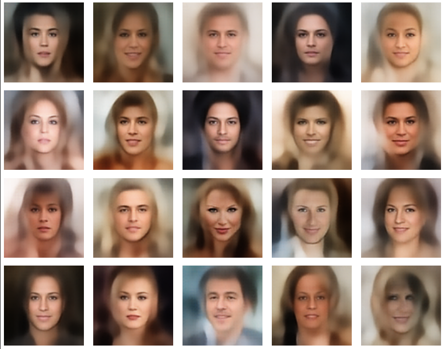
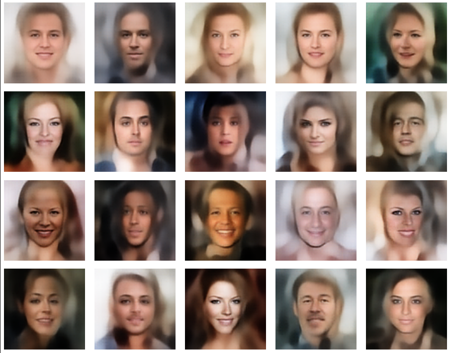
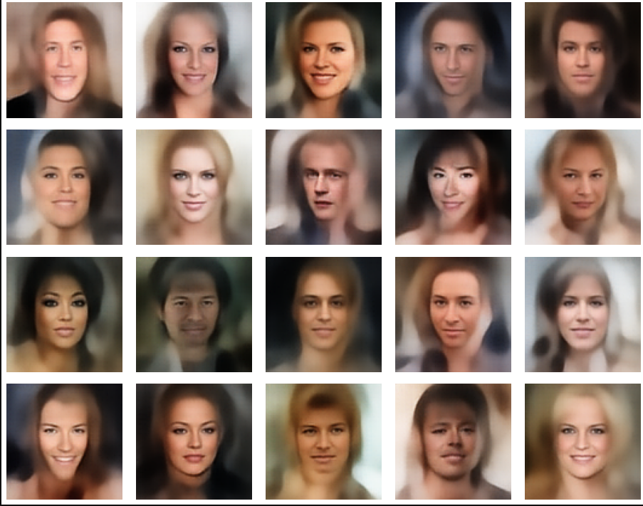
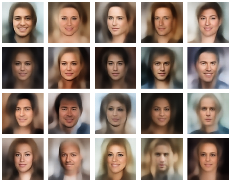
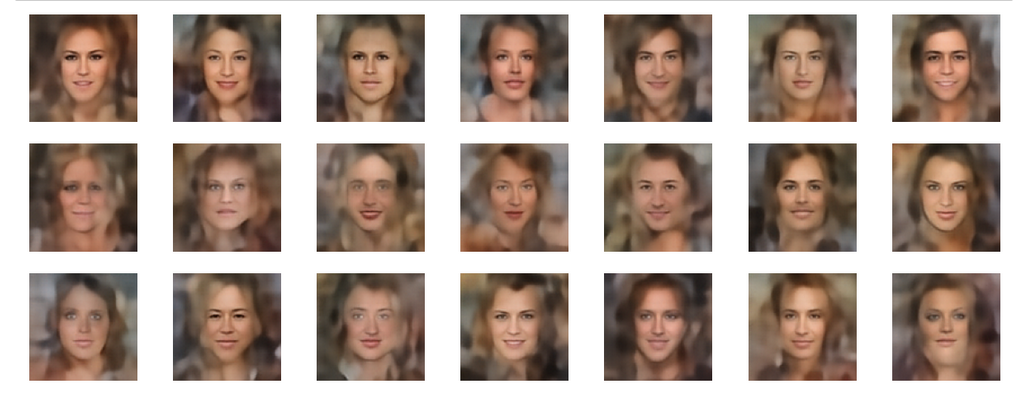
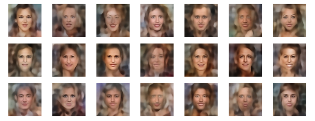
In some cases – for a higher number of PCA components – we even see smaller details of the face images and a reasonable transition to some kind of hairdo. Please remember that z_dim = 256 is a pretty low number for the latent space to cover the encoding of face details. And celebrities as covered by CelebA use make-up ….
In case you think the above result is not noteworthy: Please remember that we talk about a simple standard Autoencoder and not about a Variational Autoencoder and neither about a transformer based Autoencoder. No fancy additions to cost functions or special layers. And who ever has read the very instructive book of D. Foster on “Generative Deep Learning” (1st edition, O’Reilly) may compare his images to mine. And I have used a lower resolution of the original images than D. Foster. Just to motivate people to look a bit deeper into properties of data distributions in latent spaces.
Conclusion and outlook
We have come a lot closer to our objective of using a standard minimal Autoencoder for generative purposes. On our way, we got a much deeper understanding of the vector-distribution a trained AE creates in its latent space for human face images.
The method presented in this post to create reasonable statistical z-vectors still has its limits and there is a lot of open space for improvements. Attentive readers may e.g. ask: Why did he not use confidence ellipses directly? And why not the ellipses found in the original coordinate system of the latent space? And what about micro-correlations? And are there clusters for certain properties as the hair-color, sex, smiling, etc. in the multivariate z-point distribution in the AE’s latent space?
I will discuss these topics in further posts. In the meantime keep in mind that the basic point for turning a standard Autoencoder into a generative tool is to understand how it fills its latent space.
Note also that I myself have speculated in other posts of this blog that failures of using standard AEs for generative purposes may have their ultimate reason in the micro-structure of the z-point distribution. The present results render these previous ideas of mine plain wrong.
Links to previous posts of this series
Autoencoders and latent space fragmentation – III – correlations of latent vector components
Autoencoders and latent space fragmentation – II – number distributions of latent vector components
Autoencoders and latent space fragmentation – I – Encoder, Decoder, latent space
And before we forget it: Besides the Putler in the east there is also an extremist right-wing, semi-fascistic party in Germany on a record high support level in the population of 18%. This is a party which wants to stop all sanctions against the Russian aggressor in the ongoing war in Ukraine. You see the pattern behind this? This party is presently becoming bigger in number of supporters than the government leading social democrats. So, there is more at stake at present in Europe than the war in Ukraine. We need to defend our democracies with all the means of democracies. And its time to ask for more decisive legal action against a party which already is under observation of the German internal secret service.