Recently, I tested the propagation methods of a small Python3/Numpy class for a multilayer perceptron [MLP]. I unexpectedly ran into a performance problem with OpenBlas.
The problem had to do with the required vectorized matrix operations for forward propagation – in my case through an artificial neural network [ANN] with 4 layers. In a first approach I used 784, 100, 50, 10 neurons in 4 consecutive layers of the MLP. The weight matrices had corresponding dimensions.
The performance problem was caused by extensive multi-threading; it showed a strong dependency on mini-batch sizes and on basic matrix dimensions related to the neuron numbers per layer:
- For the given relatively small number of neurons per layer and for mini-batch sizes above a critical value (N > 255) OpenBlas suddenly occupied all processor cores with a 100% work load. This had a disastrous impact on performance.
- For neuron numbers as 784, 300, 140, 10 OpenBlas used all processor cores with a 100% work load right from the beginning, i.e. even for small batch sizes. With a seemingly bad performance over all batch sizes – but decreasing somewhat with large batch sizes.
This problem has been discussed elsewhere with respect to the matrix dimensions relevant for the core multiplication and summation operations – i.e. the neuron numbers per layer. However, the vectorizing aspect of matrix multiplications is interesting, too:
One can imagine that splitting the operations for multiple independent test samples is in principle ideal for multi-threading. So, using as many processor cores as possible (in my case 8) does not look like a wrong decision of OpenBlas at first.
Then I noticed that for mini-batch sizes “N” below a certain number (N < 250) the system only seemed to use up to 3-4 cores; so there remained plenty of CPU capacity left for other tasks. Performance for N < 250 was better by at least a factor of 2 compared to a situation with an only slightly bigger batch size (N ≥ 260). I got the impression that OpenBLAS under certain conditions just decides to use as many threads as possible – which no good outcome.
In the last years I sometimes had to work with optimizing multi-threaded database operations on Linux systems. I often got the impression that you have to be careful and leave some CPU resources free for other tasks and to avoid heavy context switching. In addition bottlenecks appeared due to the concurrent access of may processes to the CPU cache. (RAM limitations were an additional factor; but this should not be the case for my Python program.) Furthermore, one should not forget that Python/Numpy experiments on Jupyter notebooks require additional resources to handle the web page output and page update on the browser. And Linux itself also requires some free resources.
So, I wanted to find out whether reducing the number of threads – or available cores – for Numpy and OpenBlas would be helpful in the sense of an overall gain in performance.
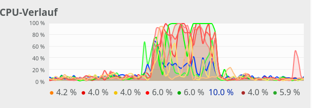
All data shown below were gathered on a desktop system with some background activity due to several open browsers, clementine and pulse-audio as active audio components, an open mail client (kontact), an open LXC container, open Eclipse with Pydev and open ssh connections. Program tests were performed with the help of Jupyter notebooks. Typical background CPU consumption looks like this on Ksysguard:

Most of the consumption is due to audio. Small spikes on one CPU core due to the investigation of incoming mails were possible – but always below 20%.
Basics
One of
the core ingredients to get an ANN running are matrix operations. More precisely: multiplications of 2-dim Numpy matrices (weight matrices) with input vectors. The dimensions of the weight matrices reflect the node-numbers of consecutive ANN-layers. The dimension of the input vector depends on the node number of the lower of two neighbor layers.
However, we perform such matrix operations NOT sequentially sample for sample of a collection of training data – we do it vectorized for so called mini-batches consisting of between 50 and 600000 individual samples of training data. Instead of operating with a matrix on just one feature vector of one training sample we use matrix multiplications whereby the second matrix often comprises many vectors of data samples.
I have described such multiplications already in a previous blog article; see Numpy matrix multiplication for layers of simple feed forward ANNs.
In the most simple case of an MLP with e.g.
- an input layer of 784 nodes (suitable for the MNIST dataset),
- one hidden layer with 100 nodes,
- another hidden layer with 50 nodes
- and an output layer of 10 nodes (fitting again the MNIST dataset)
and “mini”-batches of different sizes (between 20 and 20000). An input vector to the first hidden layer has a dimension of 100, so the weight matrix creating this input vector from the “output” of the MLP’s input layer has a shape of 784×100. Multiplication and summation in this case is done over the dimension covering 784 features. When we work with mini-batches we want to do these operations in parallel for as many elements of a mini-batch as possible.
All in all we have to perform 3 matrix operations
(784×100) matrix on (784)-vector, (100×50) matrix on (100)-vector, (50×10) matrix on (50) vector
on our example ANN with 4 layers. However, we collect the data for N mini-batch samples in an array. This leads to Numpy matrix multiplications of the kind
(784×100) matrix on an (784, N)-array, (100×50) matrix on an (100, N)-array, (50×10) matrix on an (50, N)-array.
Thus, we deal with matrix multiplications of two 2-dim matrices. Linear algebra libraries should optimize such operations for different kinds of processors.
The reaction of OpenBlas to an MLP with 4 layers comprising 784, 100, 50, 10 nodes
On my Linux system Python/Numpy use the openblas-library. This is confirmed by the output of command “np.__config__.show()”:
openblas_info:
    libraries = ['openblas', 'openblas']
    library_dirs = ['/usr/local/lib']
    language = c
    define_macros = [('HAVE_CBLAS', None)]
blas_opt_info:
    libraries = ['openblas', 'openblas']
    library_dirs = ['/usr/local/lib']
    language = c
    define_macros = [('HAVE_CBLAS', None)]
openblas_lapack_info:
    libraries = ['openblas', 'openblas']
    library_dirs = ['/usr/local/lib']
    language = c
    define_macros = [('HAVE_CBLAS', None)]
lapack_opt_info:
    libraries = ['openblas', 'openblas']
    library_dirs = ['/usr/local/lib']
    language = c
    define_macros = [('HAVE_CBLAS', None)]
and by
(ml1) myself@mytux:/projekte/GIT/ai/ml1/lib64/python3.6/site-packages/numpy/core> ldd  _multiarray_umath.cpython-36m-x86_64-linux-gnu.so
        linux-vdso.so.1 (0x00007ffe8bddf000)
        libopenblasp-r0-2ecf47d5.3.7.dev.so => /projekte/GIT/ai/ml1/lib/python3.6/site-packages/numpy/core/./../.libs/libopenblasp-r0-2ecf47d5.3.7.dev.so (0x00007fdd9d15f000)
        libm.so.6 => /lib64/libm.so.6 (0x00007fdd9ce27000)
        libpthread.so.0 => /lib64/libpthread.so.0 (0x00007fdd9cc09000)
        libc.so.6 => /lib64/libc.so.6 (0x00007fdd9c84f000)
        /lib64/ld-
linux-x86-64.so.2 (0x00007fdd9f4e8000)
        libgfortran-ed201abd.so.3.0.0 => /projekte/GIT/ai/ml1/lib/python3.6/site-packages/numpy/core/./../.libs/libgfortran-ed201abd.so.3.0.0 (0x00007fdd9c555000)
In all tests discussed below I performed a series of calculations for different batch sizes
N = 50, 100, 200, 250, 260, 500, 2000, 10000, 20000
and repeated the full forward propagation 30 times (corresponding to 30 epochs in a full training series – but here without cost calculation and weight adjustment. I just did forward propagation.)
In a first experiment, I did not artificially limit the number of cores to be used. Measured response times in seconds are indicated in the following plot:
Runtime for a free number of cores to use and different batch-sizes N
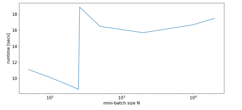
We see that something dramatic happens between a batch size of 250 and 260. Below you see the plots for CPU core consumption for N=50, N=200, N=250, N=260 and N=2000.
N=50:

N=200:

N=250:
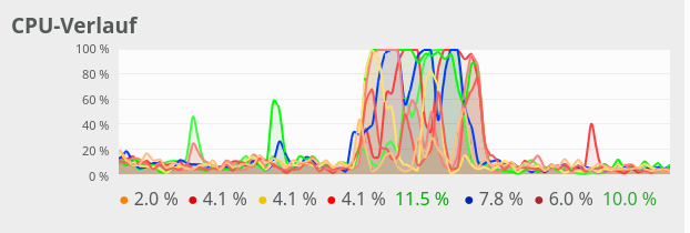
N=260:

N=2000:
The plots indicate that everything goes well up to N=250. Up to this point around 4 cores are used – leaving 4 cores relatively free. After N=260 OpenBlas decides to use all 8 cores with a load of 100% – and performance suffers by more than a factor of 2.
This result support the idea to look for an optimum of the number of cores “C” to use.
The reaction of OpenBlas to an MLP with layers comprising 784, 300, 140, 10 nodes
For a MLP with neuron numbers (784, 300, 140, 10) I got the red curve for response time in the plot below. The second curve shows what performance is possible with just using 4 cores:
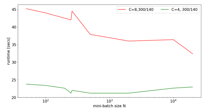
Note the significantly higher response times. We also see again that something strange happens at the change of the batch-size from 250 to 260.
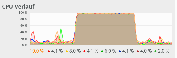
The 100% CPU
consumption even for a batch-size of only 50 is shown below:
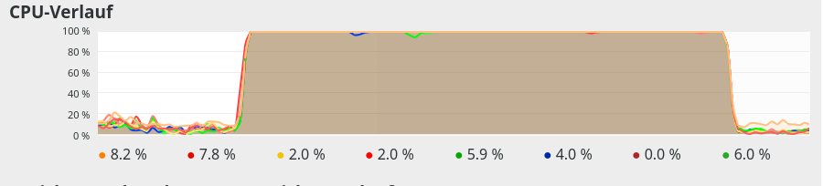
Though different from the first test case also these plots indicate that – somewhat paradoxically – reducing the number of CPU cores available to OpenBlas could have a performance enhancing effect.
Limiting the number of available cores to OpenBlas
A bit of Internet research shows that one can limit the number of cores to use by OpenBlas e.g. via an environment variable for the shell, in which we start a Jupyter notebook. The relevant command to limit the number of cores “C” to 3 is :
export OPENBLAS_NUM_THREADS=3
Below you find plots for the response times required for the batch sizes N listed above and core numbers of
C=1, C=2, C=3, C=4, C=5, C=6, C=7, C=8 :
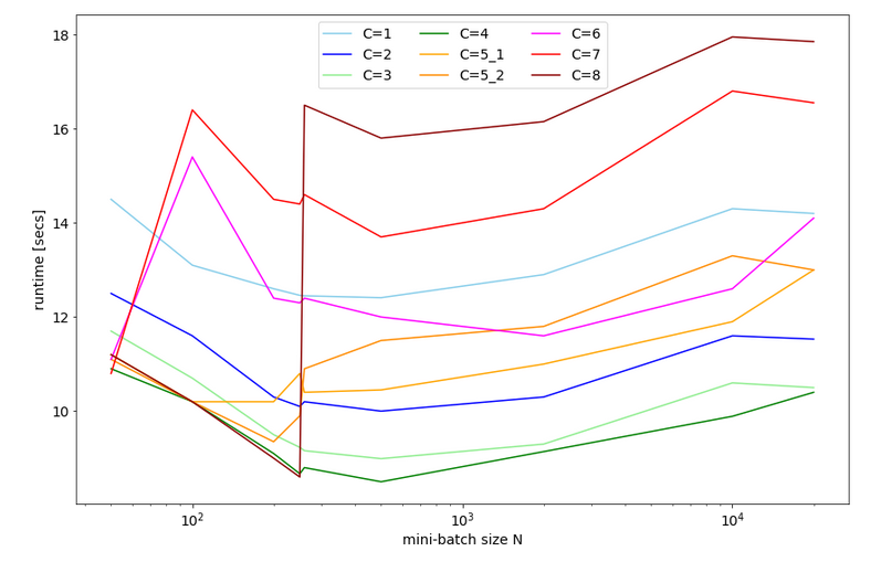
For C=5 I did 2 different runs; the different results for C=5 show that the system reacts rather sensitively. It changes its behavior for larger core number drastically.
We also find an overall minimum of the response time:
The overall optimum occurs for 400 < N < 500 for C=1, 2, 3, 4 – with the minimum region being broadest for C=3. The absolute minimum is reached on my CPU for C=4.
We understand from the plots above that the number of cores to use become hyper-parameters for the tuning of the performance of ANNs – at least as long as a standard multicore-CPU is used.
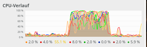
CPU-consumption
CPU consumption for N=50 and C=2 looks like:
For comparison see the CPU consumption for N=20000 and C=4:
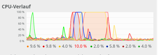
CPU consumption for N=20000 and C=6:
We see that between C=5 and C=6 CPU resources get heavily consumed; there are almost no reserves left in the Linux system for C ≥ 6.
Dependency on the size of the weight-matrices and the node numbers
For a full view on the situation I also looked at the response time variation with node numbers for a given number of CPU cores.
For C=4 and node number cases
- 784, 300, 140, 10
- 784, 200, 100, 10
- 784, 100, 50, 10
- 784, 50, 20, 10
I got the following results:
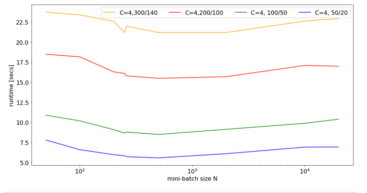
There is some broad variation with the weight-matrix size; the bigger the weight-matrix the longer the calculation time. This is, of course, to be expected. Note that the variation with the batch-size number is relatively smooth – with an optimum around 400.
Now, look at the same plot for C=6:
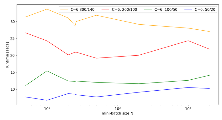
Note that the response time is significantly bigger in all cases compared to the previous situation with C=4. In cases of a large matrix by around 36% for N=2000. Also the variation with batch-size is more pronounced.
Still, even with 6 cores you do not get factors between 1.4 and 2.0 as compared to the case of C=8 (see above)!
Conclusion
As I do not know what the authors of OpenBlas are doing exactly, I refrain from technically understanding and interpreting the causes of the data shown above.
However, some consequences seem to be clear:
- It is a bad idea to provide all CPU cores to OpenBlas – which unfortunately is the default.
- The data above indicate that using only 4 out of 8 core threads is reasonable to get an optimum performance for vectorized matrix multiplications on my CPU.
- Not leaving at least 2 CPU cores free for other tasks is punished by significant performance losses.
- When leaving the decision of how many cores to use to OpenBlas a critical batch-size may exist for which the performance suddenly breaks down due to heavy multi-threading.
Whenever you deal with ANN or MLP simulations on a standard CPU (not GPU!) you should absolutely care about how many cores and related threads you want to offer to OpenBlas. As far as I understood from some Internet articles the number of cores to be used can be not only be controlled by Linux (shell) environment variables but also by os-commands in a Python program. You should perform tests to find optimum values for your CPU.
Links
stackoverflow: numpy-suddenly-uses-all-cpus
stackoverflow: run-openblas-on-multicore
stackoverflow: multiprocessing-pool-makes-numpy-matrix-multiplication-slower
scicomp: why-isnt-my-matrix-vector-multiplication-scaling/1729
Setting the number of threads via Python
stackoverflow:
set-max-number-of-threads-at-runtime-on-numpy-openblas
codereview.stackexchange: better-way-to-set-number-of-threads-used-by-numpy