Numpy matrix multiplication for layers of simple feed forward ANNs

I move a small step forward on my trials as a beginner in machine learning. This is once again going to be an article from which experts on “Artificial Neural networks” [ANNs] will learn nothing new. But some of my readers may also be newbies both to Python, to numpy and to ANNs. For them this article may be helpful.

I shall have a brief look at some matrix (or array) operations which constitute important parts of the information propagation on ANNs. How would such operations look like in Python with Numpy? One should have a clear understanding of the so called “dot”-operation between multidimensional arrays in this context. Such operations can be performed highly optimized on GPUs – and whole sets of data samples can be handled in form of vectorized code instructions. I will try to explain this in form of matrix terms required to simulate information transport between some layers of a very simple network.

Propagation operations on ANNs

Basic Artificial Neural Networks consist of layers with neurons. Each layer has a defined number of neurons. Each neuron is connected with all neurons of the next layer (receiving neurons). The output “O(k, L)” of a neuron N(k,L) of Layer “L” to a neuron N(m,L+1) is multiplied by some “weight” W[(m, L+1),(k, L),].

The contributions of all neurons on layer “L” to N(m, L+1) are summed up. The result is then transformed by some local “activation” function and afterwards presented by N(m, L+1) as output which shall be transported to the neurons of layer L+2. The succession of such operations is called “propagation“.

At the core of propagation we, therefore, find operations which we can express in the following form :

Input vector at N(m, L+1) : I(m, L+1) = SUM(over_all_k) [ W[(m, L+1), (k, L)] * O(k, L) ]
Output vector at N(m, L+1) : O(m, L+1) = f_act( I(m, L+1) )

To make things simpler: Let us set f_act = 1. Then we get

O(m, L+1) = SUM(over all k) [ W[(m, L+1), (k,N)] * O(k, L) ]

The SUM is basically a matrix operations on vector O(k, L). If output vectors were always given by singular values in “k” rows (!) then we could write

O(L+1) = W(L, L+1) * O(L) )

Batches and numerical optimization of the matrix operations for propagation

In the past I have programmed gas flow simulations in exploding stars in Fortran/C and simulated cascaded production networks for Supply Chains in PHP. There, you work with deep and complicated layer structures, too. Therefore I felt well prepared for writing a small program to set up a simple artificial neural network with some hidden layers.

Something, you will find in literature (e.g. in the book of S. Rashka, “Python machine Learning”, 2016, PACKT Publishing] are remarks on batch based training. Rashka e.g. rightfully claims in his discussion of an example code that the use of mini-batches of input data sets is advantageous (see chapter 12, page 379 in the book mentioned above):

“Mini-batch learning has the advantage over online learning that we can make use of our vectorized implementations to improve computational efficiency.”

I swallowed this remark first without much thinking. As a physicist I had used highly optimized libraries for Linear Algebra operation on supercomputers with vector registers already 35 years ago. Ok, numpy can perform a matrix operation on some vector very fast, especially on GPUs – so what?

But when I tried to follow the basic line of programming of
Rashka for an ANN in Python, I suddenly found that I did not fully understand what the code was doing whilst handling batches of input data sets. The reason was that I had not at all grasped the full implications of the quoted remark. It indicated not just the acceleration of a matrix operation on one input vector; no, instead, it indicated that we could and should perform matrix operations in parallel on all input vectors given by a full series of many different data sets in a mini-batch collection.

So, we then want to perform an optimized matrix operation on another matrix of at least 2 dimensions. When you think about it, you will quickly understand that any kind of operation of one n-dim matrix on another matrix with more and different dimensions must be defined very precisely to avoid misunderstandings and miscalculations.

To make things simple:
Let us take a (3,5)-matrix A and a (10,3)-matrix B. What should a “dot“-like operation A * B mean in this case? Would it be suitable at all, regarding the matrix element arrangements in rows and columns?

I studied the numpy documentation on “numpy.dot(A, B)”. See e.g. here. Ooops, not fully trivial: “If A is an N-D array and B is an M-D array (where M>=2), it is a sum product over the last axis of A and the second-to-last axis of B”. The matrices must obviously be arranged in a suitable way ….

So, I decided to performing some simple matrix experiments to get a clear understanding. I assumed a fictitious ANN of three layers and some direct propagation between the layers. What does propagation mean in such a case, how is it expressed in matrix operation terms in Python and what does batch-handling mean in this context?

Three simple layers and a batch of input data sets

The following graphics shows my simple network:

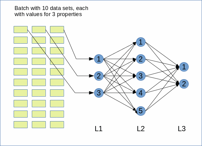
Our batch has 10 data sets of test data for our ANN. Each data set describes 3 properties; thus the input layer “L1” has 3 nodes. Our “hidden” layer “L2” shall have 5 nodes and our output layer “L3” only 2 nodes.

Weight matrices and propagation operations

Now, let us define some simple matrices with input vectors for transportation and weight-matrices for the layer-connections with Python. All activation functions shall in our simple example just perform a multiplication by 1.

The input to layer “L1” – i.e. a batch of 10 data sets – shall be given by a matrix of 10 lines (dimension 1) and 3 columns (dimension 2)

import numpy as np
import scipy
import time 

A1 = np.ones((10,3))
A1[:,1] *= 2
A1[:,2] *= 4
print("\nMatrix of input vectors to layer L1:\n")
print(A1)


print("\nMatrix of input vectors to layer 1:\n")
print(A1)

Matrix of input vectors to layer 1:

Matrix of input vectors to layer L1:

[[1. 2. 4.]
 [1. 2. 4.]
 [1. 2. 4.]
 [1. 2. 4.]
 [1. 2. 4.]
 [1. 2. 4.]
 [1. 2. 4.]
 [1. 2. 4.]
 [1. 2. 4.]
 [1. 2. 4.]]

We now define the weight matrixW1” for transport between layer L1 and layer L2 as:

W1= np.random.randint(1, 10, 5*3)
W1 = w1.reshape(5,3)
print("\nMatrix of weights W1(L1, L2) :\n")
print(W1)

Matrix of weights W1(L1, L2) :

[[3 8 5]
 [4 9 7]
 [4 1 3]
 [8 8 4]
 [3 1 9]]


We set the first dimension to the number of nodes in the target layer (L2) and the second dimension to
the number of nodes in the lower preceding layer (here: L1). Expressed in the shape notation for an array “(dimension 1, dimension 2, …) “:

Shape of W : (dim 1, dim 2) = (node number of target layer, node number of preceding layer)

If we now tried a numpy “dot”-operation for our matrices

A2 = np.dot(W1, A1)

we would get an error:

ValueError: shapes (5,3) and (10,3) not aligned: 3 (dim 1) != 10 (dim 0)

Well, this is actually consistent with the numpy documentation: The last dimension of “W1” should be consistent with the second to last (=first) dimension of “strong>A1“.

What we need to do here is to transpose the matrix of our input vectors for our multiple data sets:

A1 = np.transpose(A1)
print("\nMatrix of output vectors of layer 1 to layer 2:\n")
print(A1)

Matrix of output vectors of layer 1 to layer 2:

[[1. 1. 1. 1. 1. 1. 1. 1. 1. 1.]
 [2. 2. 2. 2. 2. 2. 2. 2. 2. 2.]
 [4. 4. 4. 4. 4. 4. 4. 4. 4. 4.]]

Then

A2 = np.dot(W1, A1)
print("\n\nA2:\n")
print(A2)

A2:

[[39. 39. 39. 39. 39. 39. 39. 39. 39. 39.]
 [50. 50. 50. 50. 50. 50. 50. 50. 50. 50.]
 [18. 18. 18. 18. 18. 18. 18. 18. 18. 18.]
 [40. 40. 40. 40. 40. 40. 40. 40. 40. 40.]
 [41. 41. 41. 41. 41. 41. 41. 41. 41. 41.]]

Now, we need a weight matrix W2 between layer L1 and layer L2:

W2= np.random.randint(1, 3, 2*5)
W2 = W2.reshape(2,5)
print("\n\nW2:\n")
print(W2)

W2:
[[2 2 1 2 2]
 [2 2 2 2 1]]

We followed the same policy – and used the number of nodes in target layer L2 as the first dimension of the weight array.

Now, do we have to to anything with array A2, if we want to use it as an input for the next matrix operation ?

A3 = np.dot(W2, A2)

No, we do not need to change anything! “A2” has the required form, already. The second to last dimension in “A2” is 5 in our example – as is the last dimension in “W2“!

So, the following will work directly :

A3 = np.dot(W2, A2)
print("\n\nA3:\n")
print(A3)

A3:

[[358. 358. 358. 358. 358. 358. 358. 358. 358. 358.]
 [335. 335. 335. 335. 335. 335. 335. 335. 335. 335.]]

You can try out our complete “propagation” code in a Jupyter notebook cell.

import numpy as np
import scipy
import time 

A1 = np.ones((10,3))
A1[:,1] *= 2
A1[:,2] *= 4
print("\nMatrix of input vectors to layer L1:\n")
print(A1)


W1= np.random.randint(1, 10, 5*3)
W1 = W1.reshape(5,3)
print("\nMatrix of weights W1(L1, L2) :\n")
print(W1)

A1 = np.transpose(A1)
print("\nMatrix of output vectors of layer L1 to layer L2:\n")
print(A1)

A2 = np.dot(W1, A1)
print("\n\nA2:\n")
print(A2)

W2= np.random.randint(1, 3, 2*5)
W2 = W2.reshape(2,5)
print("\n\nW2:\n")
print(W2)

A3 = np.dot(W2, A2)
print("\n\nA3:\n")
print(A3)

Conclusion

The first thing we learned is that matrix operations on simple vectors can be extended to a set of vectors, i.e. a matrix. In the case of ANNs one dimension of such an (numpy) array would cover the number of data sets of a typical input mini-batch. The other dimension would cover the “properties” of the input data.

The second thing we saw is that the input matrix to an ANN often must be transposed to work together with weight matrices, if such matrices follow the policy that the first dimension is given by the number of cells in the target layer and the second dimension by the number of nodes of the
preceding layer.

The weighted input to the first target layer is then given by a matrix “dot”-operation on the transposed input matrix. The outcome is a matrix where the first dimension is defined by the number of nodes of the target layer and the second dimension the number of data sets. This has already the correct form for a further propagation to the next layer. Note that the application of an activation function to each of the matrix elements would not change the required arrangement of matrix data!

After the input layer we, therefore, can just continue to directly apply weight matrices to output matrices by a numpy-“dot”-operation. The weight matrix structure just should reflect our shape policy of

(dim1, dim2) = (node number of target layer, node number of preceding layer)

.

In the next articles we shall use these insights to build a Python class for the setup and training of a simple ANN with one or two hidden layers for the analysis of the famous MNIST dataset.

Nvidia GPU-support of Tensorflow/Keras on Opensuse Leap 15

When you start working with Google’s Tensorflow on multi-layer and “deep learning” artificial neural networks the performance of the required mathematical operations may sooner or later become important. One approach to better performance is the use of a GPU (or multiple GPUs) instead of a CPU. Personally, I am not yet in a situation where GPU support is really required. My experimental CNNs are too small, yet. But starting with Keras and Tensorflow is a good point to cover the use of a GPU on my Opensuse Leap 15 systems anyway. Actually, it is also helpful for some tasks in security related environments, too. One example is testing the quality of passphrases for encryption. With JtR you may gain a factor of 10 in performance. It is interesting, how much faster an old 960 GTX card will be for a simple Tensorflow test application than my i7 CPU.

I have used Nvidia GPUs almost all my Linux life. To get GPU support for Nvidia graphics cards you need to install CUDA in its present version. This is 10.1 in August 2019. You get download and install information for CUDA at
https://developer.nvidia.com/cuda-zone => https://developer.nvidia.com/cuda-downloads
For an RPM for the x86-64 architecture and Opensuse Leap see:
https://developer.nvidia.com/cuda-downloads?….

Installation of “CUDA” and “cudcnn”

You may install the downloaded RPM (in my “case cuda-repo-opensuse15-10-1-local-10.1.168-418.67-1.0-1.x86_64.rpm”) via YaST. After this first step you in a second step install the meta-packet named “cuda”, which is available in YaST at this point. Or just install all other packets with “cuda” in the name (with the exception of the source code and dev-packets) via YaST.

A directory “/usr/local/cuda” will be built; its entries are soft links to files in a directory “/usr/local/cuda-10.1“.

Note the “include” and the “lib64” sub-directories! After the installation, also links should exist in the central “/usr/lib64“-directory pointing to the files in “/usr/local/cuda/lib64“.

Note from the file-endings that the particular present version [Aug. 2019) of the files may be something like “10.1.168“.

Another important point is that you need to install “cudnn” (cudnn-10.1-linux-x64-v7.6.2.24.tgz) – a Nvidia specific library for certain Deep Learning program elements, which shall be executed on Nvidia GPU chips. You get these files via “https://developer.nvidi.com/cudnn“. Unfortunately, you must become member of the Nvidia developer community to get access to these special files. After you downloaded the tgz-file and expanded it, you find some directories “include” and “lib64” with relevant files. You just copy these files (as user root) into the directories “/usr/local/cuda/include” and “/usr/local/cuda/lib64”, respectively. Check the owner/group and rights of the copied files afterwards and change them to root/root and standard rights – just as given for the other files in teh target directories.

The final step is the follwoing:
Create links by dragging the contents of “/usr/local/cuda/include” to “/usr/include” and chose the option “Link here”. Do the same for the files of “/usr/local/cuda/lib64” with “/usr/lib64” as the target directory. If you look at the link-directories of the files now in “usr/include” and “usr/lib64” you see exactly which files were given by the CUDA and cudcnn installation.

nAdditional libraries
In case you want to use Keras it is recommended to install the “openblas” libraries including the development packages on the Linux OS level. On an Opensuse system just search for packages with “openblas” and install them all. The same is true for the h5py-libraries. In your virtual python environment execute:
< p style="margin-left:50px;"pip3 install --upgrade h5py

Problems with errors regarding missing CUDA libraries after installation

Two stupid things may happen after this straight-forward installation :

  • The link structure between “/usr/lib64” and the files in “/usr/local/cuda/include” and “/usr/local/cuda/lib64” may be incomplete.
  • Although there are links from files as “libcufftw.so.10” to something like “libcufftw.so.10.1.168” some libraries and TensorFlow components may expect additional links as “libcufftw.so.10.0” to “libcufftw.so.10.1.168”

Both points lead to error messages when I tried to use GPU related test statements on a PyDEV console or Jupyter cell. Watch out for error messages which tell you about errors when opening specific libraries! In the case of Jupyter you may find such messages on the console or terminal window from which you started your test.

A quick remedy is to use a file-manager as “dolphin” as user root, mark all files in “/usr/local/cuda/include” and “usr/local/cuda/lib64” and place them as (soft) links into “/usr/include” and “/usr/lib64”, respectively. Then create additional links there for the required libraries “libXXX.so.10.0” to “libXXX.so.10.1.168“, where “XXX” stands for some variable part of the file name.

A simple test with Keras and the mnist dataset

I assume that you have installed the packages for tensorflow, tensorflow-gpu (!) and keras with pip3 in your Python virtualenv. Note that the package “tensorflow-gpu” MUST be installed after “tensorflow” to make the use of the GPU possible.

Then a test with a simple CNN for the “mnist” datatset can deliver information on performance differences :

Cell 1 of a Jupyter notebook:

import time 
import tensorflow as tf
from keras import backend as K
from tensorflow.python.client import device_lib
from keras.datasets import mnist
from keras import models
from keras import layers
from keras.utils import to_categorical

# function to provide CPU/GPU information 
# ---------------------------------------
def get_CPU_GPU_details():
    print("GPU ? ", tf.test.is_gpu_available())
    tf.test.gpu_device_name()
    print(device_lib.list_local_devices())

# information on available CPUs/GPUs
# --------------------------------------
if tf.test.is_gpu_available(
    cuda_only=False,
    min_cuda_compute_capability=None):
    print ("GPU is available")
get_CPU_GPU_details()

# Setting a parameter GPU or CPU usage 
#--------------------------------------
#gpu = False 
gpu = True
if gpu: 
    GPU = True;  CPU = False; num_GPU = 1; num_CPU = 1
else: 
    GPU = False; CPU = True;  num_CPU = 1; num_GPU = 0
num_cores = 6

# control of GPU or CPU usage in the TF environment
# -------------------------------------------------
# See the literature links at the article's end for more information  

config = tf.ConfigProto(intra_op_parallelism_threads=num_cores,
                        inter_op_parallelism_threads=num_cores, 
                        allow_soft_placement=True,
                        device_count = {'CPU' : num_CPU,
                                        'GPU' : num_GPU}, 
                        log_device_placement=True

                       )
config.gpu_options.per_process_gpu_memory_
fraction=0.4
config.gpu_options.force_gpu_compatible = True
session = tf.Session(config=config)
K.set_session(session)

#--------------------------
# Loading the mnist datatset via Keras 
#--------------------------
(train_images, train_labels), (test_images, test_labels) = mnist.load_data()
network = models.Sequential()
network.add(layers.Dense(512, activation='relu', input_shape=(28*28,)))
network.add(layers.Dense(10, activation='softmax'))
network.compile(optimizer='rmsprop', loss='categorical_crossentropy', metrics=['accuracy'])
train_images = train_images.reshape((60000, 28*28))
train_images = train_images.astype('float32') / 255
test_images = test_images.reshape((10000, 28*28))
test_images = test_images.astype('float32') / 255
train_labels = to_categorical(train_labels)
test_labels = to_categorical(test_labels)

Output of the code in cell 1:

GPU is available
GPU ?  True
[name: "/device:CPU:0"
device_type: "CPU"
memory_limit: 268435456
locality {
}
incarnation: 17801622756881051727
, name: "/device:XLA_GPU:0"
device_type: "XLA_GPU"
memory_limit: 17179869184
locality {
}
incarnation: 6360207884770493054
physical_device_desc: "device: XLA_GPU device"
, name: "/device:XLA_CPU:0"
device_type: "XLA_CPU"
memory_limit: 17179869184
locality {
}
incarnation: 7849438889532114617
physical_device_desc: "device: XLA_CPU device"
, name: "/device:GPU:0"
device_type: "GPU"
memory_limit: 2115403776
locality {
  bus_id: 1
  links {
  }
}
incarnation: 4388589797576737689
physical_device_desc: "device: 0, name: GeForce GTX 960, pci bus id: 0000:01:00.0, compute capability: 5.2"
]

Note the control settings for GPU usage via the parameter gpu and the variable “config”. If you do NOT want to use the GPU execute

config = tf.ConfigProto(device_count = {‘GPU’: 0, ‘CPU’ : 1})

Information on other control parameters which can be used together with “tf.ConfigProto” is provided here:
https://stackoverflow.com/questions/40690598/can-keras-with-tensorflow-backend-be-forced-to-use-cpu-or-gpu-at-will

Cell 2 of a Jupyter notebook for performance measurement during training:

start_c = time.perf_counter()
with tf.device("/GPU:0"):
    network.fit(train_images, train_labels, epochs=5, batch_size=30000)
end_c = time.perf_counter()
if CPU: 
    print('Time_CPU: ', end_c - start_c)  
else:  
    print('Time_GPU: ', end_c - start_c)  

Output of the code in cell 2 :

Epoch 1/5
60000/60000 [==============================] - 0s 3us/step - loss: 0.5817 - acc: 0.8450
Epoch 2/5
60000/60000 [==============================] - 0s 3us/step - loss: 0.5213 - acc: 0.8646
Epoch 3/5
60000/60000 [==============================] - 0s 3us/step - loss: 0.4676 - acc: 0.8832
Epoch 4/5
60000/60000 [==============================] - 0s 3us/step - loss: 0.4467 - acc: 0.8837
Epoch 5/5
60000/60000 [==============================] - 0s 3us/step - loss: 0.4488 - acc: 0.8726
Time_GPU:  0.7899935730001744

Now change the following lines in cell 1

 
...
gpu = False 
#gpu = True 
...

Executing the code in cell 1 and cell 2 then gives:

Epoch 1/5
60000/60000 [==============================] - 0s 6us/step - loss: 0.4323 - acc: 0.8802
Epoch 2/5
60000/60000 [==============================] - 0s 7us/step - loss: 0.3932 - acc: 0.8972
Epoch 3/5
60000/60000 [==============================] - 0s 6us/step - loss: 0.3794 - acc: 0.8996
Epoch 4/5
60000/60000 [==============================] - 0s 6us/step - loss: 0.3837 - acc: 0.8941
nEpoch 5/5
60000/60000 [==============================] - 0s 6us/step - loss: 0.3830 - acc: 0.8908
Time_CPU:  1.9326397939985327

Thus the GPU is faster by a factor of 2.375 !
At least for the chosen batch size of 30000! You should play a bit around with the batch size to understand its impact.
2.375 is not a big factor – but I have a relatively old GPU (GTX 960) and a relatively fast CPU i7-6700K mit 4GHz Taktung: So I take what I get 🙂 . A GTX 1080Ti would give you an additional factor of around 4.

Watching GPU usage during Python code execution

A CLI command which gives you updated information on GPU usage and memory consumption on the GPU is

nvidia-smi -lms 250

It gives you something like

Mon Aug 19 22:13:18 2019       
+-----------------------------------------------------------------------------+
| NVIDIA-SMI 418.67       Driver Version: 418.67       CUDA Version: 10.1     |
|-------------------------------+----------------------+----------------------+
| GPU  Name        Persistence-M| Bus-Id        Disp.A | Volatile Uncorr. ECC |
| Fan  Temp  Perf  Pwr:Usage/Cap|         Memory-Usage | GPU-Util  Compute M. |
|===============================+======================+======================|
|   0  GeForce GTX 960     On   | 00000000:01:00.0  On |                  N/A |
| 20%   44C    P0    33W / 160W |   3163MiB /  4034MiB |      1%      Default |
+-------------------------------+----------------------+----------------------+
                                                                               
+-----------------------------------------------------------------------------+
| Processes:                                                       GPU Memory |
|  GPU       PID   Type   Process name                             Usage      |
|=============================================================================|
|    0      4124      G   /usr/bin/X                                   610MiB |
|    0      4939      G   kwin_x11                                      54MiB |
|    0      4957      G   /usr/bin/krunner                               1MiB |
|    0      4959      G   /usr/bin/plasmashell                         195MiB |
|    0      5326      G   /usr/bin/akonadi_archivemail_agent             2MiB |
|    0      5332      G   /usr/bin/akonadi_imap_resource                 2MiB |
|    0      5338      G   /usr/bin/akonadi_imap_resource                 2MiB |
|    0      5359      G   /usr/bin/akonadi_mailfilter_agent              2MiB |
|    0      5363      G   /usr/bin/akonadi_sendlater_agent               2MiB |
|    0      5952      C   /usr/lib64/libreoffice/program/soffice.bin    38MiB |
|    0      8240      G   /usr/lib64/firefox/firefox                     1MiB |
|    0     13012      C   /projekte/GIT/ai/ml1/bin/python3            2176MiB |
|    0     14233      G   ...uest-channel-token=14555524607822397280    62MiB |
+-----------------------------------------------------------------------------+

During code execution some of the displayed numbers – e.g for GPU-Util, GPU memory Usage – will start to vary.

Links

https://medium.com/@liyin2015/tensorflow-cpus-and-gpus-configuration-9c223436d4ef
https://www.tensorflow.org/beta/guide/using_gpu
https://stackoverflow.com/questions/40690598/can-keras-with-tensorflow-backend-be-forced-to-use-cpu-or-gpu-at-will
https://stackoverflow.com/questions/42706761/closing-session-in-tensorflow-
doesnt-reset-graph

http://www.science.smith.edu/dftwiki/index.php/Setting up Tensorflow 1.X on Ubuntu 16.04 w/ GPU support
https://hackerfall.com/story/which-gpus-to-get-for-deep-learning
https://towardsdatascience.com/measuring-actual-gpu-usage-for-deep-learning-training-e2bf3654bcfd


Der nächste Schritt ….

Die Grenzen zur Beeinträchtigung der digitalen Privatsphäre werden (erwartungsgemäß) weiter ausgelotet:
https://www.golem.de/news/verfassungsschutz-einbruch-fuer-den-staatstrojaner-1908-143268.html
https://www.sueddeutsche.de/politik/gesetzentwurf-bundesamt-fuer-einbruch-1.4564401
Unsere Sicherheitsorgane nicht mehr nur als Hacker ?.?.? — weil Hacking wohl zu mühsam ist und (erwartungsgemäß) nicht überall zum Erfolg führt?

Als nunmehr 60-Jähriger und Werte-Konservativer wundere ich mich über gar nichts mehr. Ich habe an der Schule noch gelernt, wie essentiell eine Beschneidung der Möglichkeiten von Inlandsgeheimdiensten aufgrund der Erfahrungen aus dem sog. Dritten Reich ist – und dass es nach unserer Verfassung zu keiner Verquickung geheimdienstlicher und polizeilicher Tätigkeiten kommen solle und dürfe. Und dass ein richterlicher Beschluss unbedingte Grundlage jeder Verletzung der Privatsphäre sein muss. Nun erleben wir, wie im Namen der Sicherheit von den Bewahrern der Sicherheit “weiter” gedacht wird. Dass sich große internationale IT-Monopolisten um Privatsphäre und die dt. Verfassung bislang schon wenig scherten, überraschte wenig; von führenden Politikern und Ministerien muss man als Demokrat dagegen mehr erwarten dürfen.

Früher verhinderte die Umsetzung solcher Ideen, wie sie in den in den Artikeln behandelten Gesetzentwürfen ausgeführt werden, allein schon der Aufstand der Rechtschaffenen in der FDP und der SPD. Wo bleibt deren Aufschrei heute? Die SPD fragt sich wahrscheinlich in Arbeitskreisen auf lokaler Ebene erstmal, ob sie in einer zunehmend digitalisierten Welt überhaupt leben wolle – kein Witz, das wurde mir von einem Ortsvorstand genau so in einem Biergarten gesagt – … und wenn, ob man dafür dann nicht ein Tripel statt eines Duos für die Parteiführung benötige … Hr. Lindner von der FDP würde wohl antworten, dass man solche komplexen Themen nur und ausschließlich den Profis überlassen muss – und nicht der Parteipolitik …

Denkt man IT-Sicherheit und IT-Privatsphäre durch, so wird schnell klar, welche extreme Bedeutung der Unversehrtheit privat oder professionell genutzter IT-Systeme zukommt. Ist die nicht mehr gegeben, so gibt es schlicht und einfach gar keine Privatsphäre mehr – auch nicht bei Einsatz von auf Sicherheit getrimmten Linux-Systemen und voll-verschlüsselter System-/Daten-Platten bzw. -Partitionen oder gar der temporären Entfernung von Datenträgern aus den Systemen bei längerer Abwesenheit. Selbst wenn man als vorsichtiger Zeitgenosse (z.B. als Investigativ-Journalist) seine genutzten Linux-Betriebssysteme und seine Daten nach einer solchen längeren Abwesenheit nur aus voll-verschlüsselten Backups mit prüfbaren Hash-Summen rekonstruieren würde, die man zuvor an sicheren Orten platziert hätte, würde einen das gegenüber unbefugten Eindringlingen in Wohnung oder Home-Office nicht wirklich schützen. Da die Eindringlinge – egal welcher Coleur – ja womöglich Zugriff auf die Hardware der genutzten Systeme (wie PCs, Server) bekämen, könnten sie auch diese manipulieren. Das ist u.U. sogar einfacher und für den Betroffenen schwerer zu entdecken als Manipulationen an Software. Hatten uns die Amerikaner nicht vor kurzer Zeit genau davor im Zshg. mit Huwai und anderen chinesischen Herstellern gewarnt? Nun, das Volk der Dichter und Denker erweist sich als lernfähig. Tja, es scheint, als mangelte es selbst den Herren Huxley und Orwell an hinreichender Phantasie für die Wirklichkeit …