Hat nichts mit Linux zu tun, ist aber für alle Freiheitsliebende relevant. Nach einem Übermaß an Überflutung mit Plakaten der AfD (“Wir vergessen nicht”) und rechten Stammtischparolen in einem Kurzurlaub verweise ich ohne weiteren Kommentar auf folgenden Link:
Ich bin kein FDP-Wähler, aber wo einer der sehr wenigen verbliebenen Aufrechten in dieser Partei leider zu 100 Prozent recht hat, erhält er meine volle inhaltliche Zustimmung.
A reader wrote me a mail and asked what the general direction of this blog is going to be. He wondered about the “flood” of formulas lately. Which, in his opinion, have nothing to do with Linux. In general, his impression was that I seemingly have lost my interest in core Linux topics. He, a German, also complained that I write my posts in English.
My first reaction was: I appreciate that some of my readers care. The criticism is justified. And it deserves an answer and some explanations. The easiest part is the question regarding language.
According to my provider and my own blog-statistics 78% of page requests to this blog come from abroad, i.e. from countries outside Germany. Most requests stem from US-systems. Before Russia’s imperialistic war against Europe there also were connections (and permanent attack trials) from both Russia and China. Their percentage has declined (fortunately). Anyway, the majority of page requests comes from outside Germany. Therefore, I try to write in English. My English certainly is not the best, but it is still easier to read for those who are interested in my posts’ contents. And obviously, these are not German readers. So, I will not go back to German again.
Now to the question regarding the declining number of posts related to Linux. In the time when I worked as a free-lancer (up to 2018), I had some German customers who cared about Linux. It was in my own interest to dig a bit deeper as usual into topics like “virtualized VLANs”, firewalls etc.. The articles on these topics are still the most read ones in this blog.
But then I started to work as an employed consultant for IT-management topics in a Windows-dominated company. I simply had no chance and no time to continue with hard core Linux topics until the end of 2022. The only connection that came up was related to minor Machine Learning topics. Since my retirement I again use my private Linux systems – but what I need there simply works. No need to dig deeper at the moment. I intend to shift all of my HW-platforms and in the wake of such an endeavor typically some Linux topics come up, but all of this requires a period of money saving first. The same holds for a private project concerning central Linux-based audio-station. (Side remark: Due to the systematic destruction of the social system in Germany, ironically and mainly by the politics of social democrats, ca. 10 million of the persons going into retirement the next years will get significantly less than 1500 Euros per month. These are official numbers of the German government. I am on the edge of this wave.)
A second point which obviously has an impact on this blog is that I have an education in physics and an inborn interest in math. One of the best aspects of retirement is that you gain a lot of freedom regarding your real interests. No employer longer forces you to focus on things you only work with to earn a living. In my case the physicist woke up in spring 2023. I started to read a lot of books on theoretical physics and cosmology. To find out that I needed to revive some university level mathematics. At the same time I got interested in some admittedly special aspects of my own ML-experiments and network simulations in general. And suddenly you find yourself applying some basic linear algebra and calculus again. An easy but not very thoughtful way to start collecting some simple, but useful results was using this blog. I admit: It has turned the blog’s focus away from Linux.
The solution is clear: This blog has to be split up. I will do this as soon as I find some motivation for the boring task to set up a new blog, database, etc. For the time being I have changed the subtitle of this blog to indicate that other topics have come up.
What I cannot promise is that Linux topics will dominate my interests in the future. As said: What a retired person needs on PCs and laptops normally works perfectly under the control of Linux. Thanks to all the fantastic people of the Open Source community.
This post requires Javascript to display formulas!
A centered, rotated ellipse can be defined by matrices which operate on position-vectors for points on the ellipse. The topic of this post series is the relation of the coefficients of such matrices to some basic geometrical properties of an ellipse. In the previous posts
we have found that we can use (at least) two matrix based approaches:
One reflects a combination of two affine operations applied to a unit circle. This approach led us to a non-symmetric matrix, which we called AE. Its coefficients ((a, b), (c, d)) depend on the lengths of the ellipses’ principal axes and trigonometric functions of its rotation angle.
The second approach is based on coefficients of a quadratic form which describes an ellipse as a special type of a conic section. We got a symmetric matrix, which we called Aq.
We have shown how the coefficients α, β, γ of Aq can be expressed in terms of the coefficients of AE. Another major result was that the eigenvalues and eigenvectors of Aq completely control the ellipse’s properties.
Furthermore, we have derived equations for the lengths σ1, σ2 of the ellipse’s principal axes and the rotation angle by which the major axis is rotated against the x-axis of the Cartesian coordinate system [CCS] we work with.
We have also found equations for the components of the position vectors to those points of the ellipse with maximum y-values.
In this post we determine the components of the vectors to the end-points of the ellipse’s principal axes in terms of the coefficients of Aq. Afterward we shall test our formulas by a Python program and plots for a specific example.
Reduced matrix equation for an ellipse
Our centered, but rotated ellipse is defined by a quadratic form, i.e. by a polynomial equation with quadratic terms in the components xe and ye of position vectors to points on the ellipse:
The quadratic polynomial can be formulated as a matrix operation applied to position vectors vE = (xE, yE)T. With the the quadratic and symmetric matrix Aq
Method 1 to determine the vectors to the principal axes’ end points
My readers have certainly noticed that we have already gathered all required information to solve our task. In the first post of this series we have performed an eigendecomposition of our symmetric matrix Aq. We found that the two eigenvectors of Aq for respective eigenvalues λ1 and λ2 point along the principal axes of our rotated ellipse:
This is trivial regarding the algebraic operations, but results in lengthy (and boring) expressions in terms of the matrix coefficients. So, I skip to write down all the terms. (We do not need it for setting up ordered numerical programs.)
Remember that you could in addition replace (α, β, γ) by coefficients (a, b, c, d) of matrix AE. See the first post of this series for the formulas. This would, however, produce even longer equation terms.
We pick the yE with the positive term in the following steps. (The way for the solution with the negative term in yE is analogous.) The square of yE is:
A detailed analysis also for the other yE-expression (see above) leads to further solutions for the coordinates (=vector component values) of points with extremal values for the radii. These are the end-points of the principal axes of the ellipse:
I leave it to the reader to expand the convenience variables into terms containing the original coefficients α, β, γ.
Plots
It is easy to write a Python program, which calculates and plots the data of an ellipse and the special points with extremal values of the radii and extremal values of ye. The general steps which I followed were:
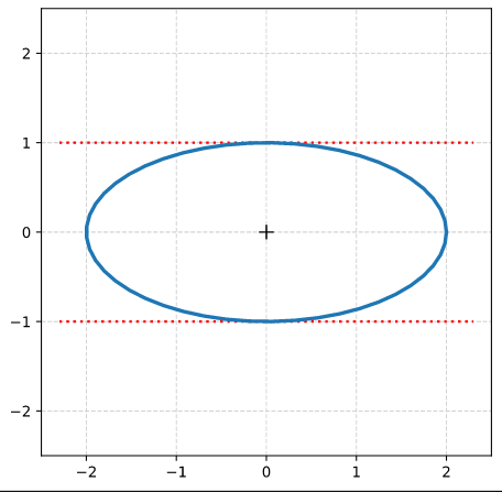
Step 0: Create 100 points a unit circle. Save the coordinates in Python lists (or Numpy arrays). Use Matplotlib’s plot(x,y)-function to plot the vectors.
Step 1: Create an axis-parallel ellipse with values for the axes ha = 2.0 and hb = 1.0 along the x- and the y-axis of the Cartesian coordinate system [CCS]. Do this by applying a diagonal scaling matrix Dσ1, σ2 (see the first post of this series).
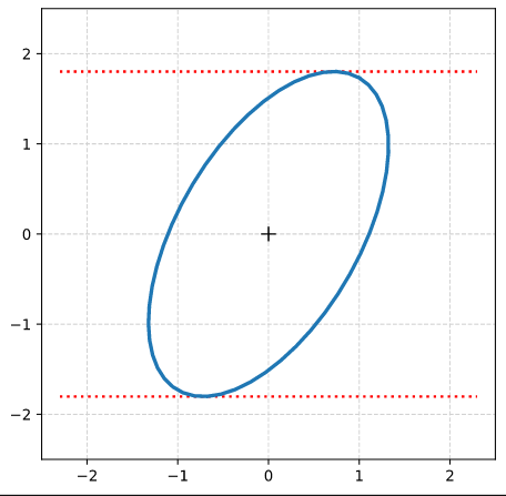
Step 2: Rotate the ellipse bei π/3 (60 °). Do this by applying a rotation matrix Rπ/3 to the position vectors of your ellipse (with the help of Numpy). Alternatively, you can first create the matrices, perform a matrix multiplication and then apply the resulting matrix to the position vectors of your unit circle.
(The limiting lines have been calculated by the formulas given above.)
Step 3: Determine the coefficients of combined matrix AE = Rπ/3 ○ Dσ1, σ2
I got for the coefficients ( (a, b), (c, d) ) of AE :
A_ell =
[[ 1.         -0.8660254 ]
[ 1.73205081  0.5       ]]
Step 3: Determine the coefficients of the matrix Aq by the formulas given in the first post of this series. I got
A_q =
[[ 3.25       -1.29903811]
[-1.29903811  1.75      ]]
For δ I got:
delta = 4.0
which is consistent with the length-values of the principal axes.
Step 4: Determine values for the eigenvalues λ1 and λ2 from the Aq-coefficients by the formulas given in the first post. Also calculate them by using Numpy’s
eigenvalues, eigenvectors = numpy.linalg.eig(A_q). Theory tells us that these values should be exactly λ1 = 4 and λ1 = 1. I got
Eigenvalues from A_q: lambda_1 = 4. :: lambda_2 = 1.
Step 5: Determine the components of the normalized eigenvectors with the help of numpy.linalg.eig(A_q). I got:
Components of normalized eigenvectors by theoretical formulas from A_q coefficients:
ev_1_n :  -0.8660254037844386  :  0.5000000000000002
ev_2_n :  0.5000000000000001  :  0.8660254037844385

Eigenvectors from A_q via numpyy.linalg.eig():
ev_1_num :  0.8660254037844387  :  -0.5000000000000001
ev_2_num :  0.5000000000000001  :  0.8660254037844387
The deviation between ev_1_n and ev_1_num is just due to a difference by -1. This is correct as the eigenvectors are unique only up to a minus-sign in all components.
Step 6: Calculate the sinus of the rotation angle of our ellipse from Aq– and Aq-coefficients. The theoretical value is sin(2 π/3) = sin(2 pi/3) = 0.8660254037844387. I got:
sin(2. * rotation angle) of major axis of the ellipse against the CCS x-axis from A_E coefficients:
sin_2phi-A_E  =  0.8660254037844388

sin(2. * rotation angle) of major axis of the ellipse against the CCS x-axis from from eigenvectors of A_q:
sin_2phi-ev_A_q =  0.8660254037844387

sin(2. * rotation angle) of major axis of the ellipse against the CCS x-axis from A_q-coefficients:
sin_2phi-coeff-A_q =  0.8660254037844388
Perfect!
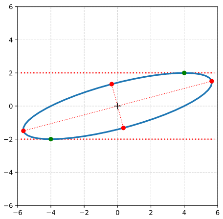
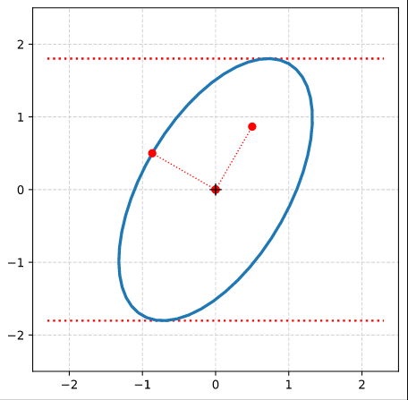
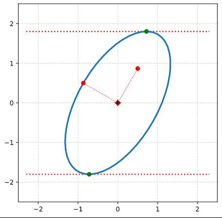
Step 7: Plot the end-points of the normalized eigenvectors of Aq:
Note that in our example case the end-point of the eigenvector along the minor axis must be located exactly on the elliptic curve as the ellipses minor axes has a length of b=1!
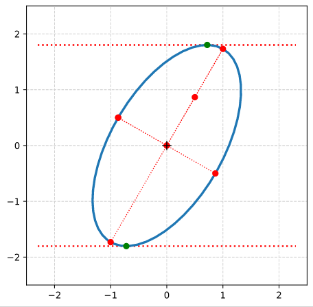
Step 8: Calculate the components of the vectors to data-points of the ellipse with maximal absolute ye-values from the Aq-coefficients given in the previous post. Plot these data-points (here in green color).
Step 9: Calculate the components of the vectors to data-points of the ellipse with maximal values of the radii with the help of the complex formulas presented in this post and plot these points in addition.
Conclusion
In this mini-series of posts we have performed some small mathematical exercises with respect to centered and rotated ellipses. We have calculated basic geometrical properties of such ellipses from the coefficients of matrices which define ellipses in algebraic form. Linear Algebra helped us to understand that the eigenvectors and eigenvalues of a symmetric matrix, whose coefficients stem from a quadratic equation (for a conic section), control both the orientation and the lengths of the ellipse’s axes completely.
This knowledge is useful in some Machine Learning [ML] context where elliptic data appear as projections of multivariate normal distributions. Multivariate Gaussian probability functions control properties of a lot of natural objects. Experience shows that certain types of neural networks may transform such data into multivariate normal distributions in latent spaces. An evaluation of the numerical data coming from such ML-experiments often delivers the coefficients of defining matrices for ellipses.
In my blog I now return to the study of with shearing operations applied to circles, spheres, ellipses and 3-dimensional ellipsoids. Later I will continue with the study of multivariate normal distributions in latent spaces of Autoencoders. For both of these topics the knowledge we have gathered regarding the matrices behind ellipses will help us a lot.
I have discussed how the coefficients of two matrices which can be used to define a centered, rotated ellipse can be used to calculate geometrical properties of the ellipse:
The lengths σ1, σ2 of the ellipse’s principal axes and the rotation angle by which the major axis is rotated against the x-axis of the Cartesian coordinate system [CCS] we work with.
But there are other properties which are interesting, too. A centered, rotated ellipse has two points with extremal values in their y-coordinates. Can we express the coordinates – or equivalently the components of respective position vectors – in terms of the basic matrix coefficients?
The answer is, of course, yes. This post provides a derivation of respective formulas.
Matrix equation for an ellipse
In the last post we have shown that a centered ellipse is defined by a quadratic form, i.e. by a polynomial equation with quadratic terms in the components xE and yE of position vectors for points of the ellipse:
The quadratic polynomial can be formulated as a matrix operation applied to position vectors vE of points on an ellipse. With the the quadratic and symmetric matrix Aq
We now follow the alternative solution for yE (see above). After a calculation of the yE-values from the derived xE values, we get the components for the two position vectors to the points with extremal y-values on the ellipse:
Solution in terms of the coefficients of an alternative matrix AE
In my previous post I have discussed yet another matrix AE which also can be used to define an ellipse. This matrix summarizes two affine transformations of a centered unit circle: AE = Rφ ○ Dσ1, σ2. Dσ1, σ2.
You find the relations between the coefficients (a, b, c, d) of matrix AE and the coefficients (α, β, γ) of matrix Aq in my previous post. This will allow you to calculate the vectors to the extremal points of an ellipse in terms of the coefficients (a, b, c, d).
Conclusion
In this post we have again used the coefficients of a matrix which defines an ellipse via a quadratic form to get information about a geometrical property.
We can now calculate the components of the position vectors to the two points of an ellipse with extremal y-values as functions of the matrix coefficients.
I will show you how to calculate the components of the end points of the principal axes of the ellipse with the help of our matrix for a quadratic form. I will also use our theoretical results for plots of some ellipses’ axes and of their extremal points. We will also compare theoretical predictions with numerically evaluated values.
some geometrical and algebraic properties of ellipses are of interest.
Geometrically, we think of an ellipse in terms of their perpendicular two principal axes, focal points, ellipticity and rotation angles with respect to a coordinate system. As elliptic data appear in many contexts of physics, chaos theory, engineering, optics … ellipses are well studied mathematical objects. So, why a post about ellipses in the Machine Learning section of a blog?
In my present working context ellipses appear as a side result of statistical multivariate normal distributions [MNDs]. The projections of multidimensional contour hyper-surfaces of a MND within the ℝn onto coordinate planes of an Cartesian Coordinate System [CCS] result in 2-dimensional ellipses. These ellipses are typically rotated against the axes of the CCS – and their rotation angles reflect data correlations. The general relations of statistical vector data with projections of multidimensional MNDs are somewhat intricate.
Data produced in numerical experiments, e.g. in a Machine Learning context, most often do not give you the geometrical properties of ellipses, which some theory may have predicted, directly. Instead you may get numerical values of statistical vector distributions which correspond to algebraic coefficients. Examples of such coefficients are e.g. correlation coefficients. These coefficients can often be regarded as elements of a matrix. In case of an underlying MND of your statistical variables these matrices indirectly and approximately describe contour surfaces – namely ellipsoids. Or regarding projections of the data on 2-dim coordinate planes “ellipses”.
Ellipsoids/ellipses can in general be defined by matrices operating on position vectors. In particular: Coefficients of quadratic polynomial expressions used to describe ellipses as conic sections correspond to the coefficients of a matrix operating on position vectors.
So, when I became confronted with multidimensional MNDs and their projections on coordinate planes the following questions became interesting:
How can one derive the lengths σ1, σ2 of the perpendicular principal axes of an ellipse from data for the coefficients of a matrix which defines the ellipse by a polynomial expression?
By which formula do the matrix coefficients provide the inclination angle of the ellipse’s primary axes with the x-axis of a chosen coordinate system?
You may have to dig a bit to find correct and reproducible answers in your math books. Regarding the resulting mathematical expressions I have had some bad experiences with ChatGPT. But as a former physicist I take the above questions as a welcome exercise in solving quadratic equations and doing some linear algebra. So, for those of my readers who are a bit interested in elementary math I want to answer the posed questions step by step and indicate how one can derive the respective formulas. The level is moderate – you need some knowledge in trigonometry and/or linear algebra.
Centered ellipses and two related matrices
Below I regard ellipses whose centers coincide with the origin of a chosen CCS. For our present purpose we thus get rid of some boring linear terms in the equations we have to solve. We do not loose much of general validity by this step: Results of an off-center ellipse follow from applying a simple translation operation to the resulting vector data. But I admit: Your (statistical) data must give you some relatively precis information about the center of your ellipse. We assume that this is the case.
Our ellipses can be rotated with respect to a chosen CCS. I.e., their longer principal axes may be inclined by some angle φ towards the x-axis of our CCS.
There are actually two different ways to define a centered ellipse by a matrix:
Alternative 1: We define the (rotated) ellipse by a matrix AE which results from the (matrix) product of two simpler matrices: AE = Rφ ○ Dσ1, σ2. Dσ1, σ2 corresponds to a scaling operation applied to position vectors for points located on a centered unit circle. Aφ describes a subsequent rotation. AE summarizes these geometrical operations in a compact form.
Alternative 2: We define the (rotated) ellipse by a matrix Aq which combines the x- and y-elements of position vectors in a polynomial equation with quadratic terms in the components (see below). The matrix defines a so called quadratic form. Geometrically interpreted, a quadratic form describes an ellipse as a special case of a conic section. The coefficients of the polynomial and the matrix must, of course, fulfill some particular properties.
While it is relatively simple to derive the matrix elements from known values for σ1, σ2 and φ it is a bit harder to derive the ellipse’s properties from the elements of either of the two defining matrices. I will cover both matrices in this post.
For many practical purposes the derivation of central elliptic properties from given elements of Aq is more relevant and thus of special interest in the following discussion.
Matrix AE of a centered and rotated ellipse: Scaling of a unit circle followed by a rotation
Our starting point is a unit circle C whose center coincides with our CCS’s origin. The components of vectors vc to points on the circle C fulfill the following conditions:
DE is a diagonal matrix which describes a stretching of the circle along the CCS-axes, and Rφ is an orthogonal rotation matrix. The stretching (or scaling) of the vector-components is done by
As we already know, σ1 and σ2 are factors which give us the lengths of the principal axes of the ellipse. σ1 and σ2 have positive values. We, therefore, can safely assume:
Ok, we have defined an ellipse via an invertible matrix AE, whose coefficients are directly based on geometrical properties.
But as said: Often an ellipse is described by a an equation with quadratic terms in x and y coordinates of data points. The quadratic form has its background in algebraic properties of conic sections. As a next step we derive such a quadratic equation and relate the coefficients of the quadratic polynomial with the elements of our matrix AE. The result will in turn define another very useful matrix Aq.
Quadratic forms – Case 1: Centered ellipse, principal axes aligned with CCS-axes
We start with a simple case. We take a so called axis-parallel ellipse which results from applying only a scaling matrix DE onto our unit circle C. I.e., in this case, the rotation matrix is assumed to be just the identity matrix. We can omit it from further calculations:
To get quadratic terms of vector components it often helps to invoke a scalar product. The scalar product of a vector with itself gives us the squared norm or length of a vector. In our case the norms of the inversely re-scaled vectors obviously have to fulfill:
I.e., we can directly derive σ1, σ2 and φ from the coefficients of the quadratic form. But an axis-parallel ellipse is a very simple ellipse. Things get more difficult for a rotated ellipse.
Quadratic forms – Case 2: General centered and rotated ellipse
We perform the same trick with the vectors vE to get a quadratic polynomial for a rotated ellipse:
Thus Aq is an invertible matrix if AE is invertible. For standard conditions (σ1 >0, σ2 > 0) this is the case (see above). Furthermore, Aq is symmetric and thus its own transposed matrix.
Above we have got α, β, γ as some relatively simple functions of a, b, c, d. The inversion is not so trivial and we do not even try it here.
Instead we focus on how we can express σ1, σ2 and φ as functions of either (a, b, c, d) or (α, β, γ).
How to derive σ1, σ2 and φ from the coefficients of AE or Aq in the general case?
Let us assume we have (numerical) data for the coefficients of the quadratic form. Then we may want to calculate values for the length of the principal axes and the rotation angle φ of the corresponding ellipse. There are two ways to derive respective formulas:
Approach 1: Use trigonometric relations to directly solve the equation system.
Approach 2: Use an eigenvector decomposition of Aq.
Both ways are fun!
Direct derivation of σ1, σ2 and φ from Aq by using trigonometric relations
Without loosing much of generality we further assume
\[
\lambda_2 \:\ge \lambda_1 \,.
\]
This affects some aspects of the following derivations and should be kept in mind whilst reading. In the end, our results would only differ by a rotation of π/2, if we had chosen otherwise.
Note, however, that due to our assumption we discuss ellipses whose half-axis σ1 in x-direction is longer than the half-axis σ2 in y-direction!
By combining the above relations for the Aq-coefficients we find
See a later section below for ambiguities coming from the arcsin-function. A proper analysis and interpretation of this formula for the rotation angle is necessary, when you want to reconstruct ellipses by numerical methods from a given matrix Aq. Some matrices may describe ellipses with their half-axis in y-direction being longer than the half-axis in x-direction. Then λ1 and λ2 would change their role with respect to x,y.
Example:
A typical example for a matrix would be one that appears in the context of a standardized (!) bivariate normal distribution with some correlation imposed onto the statistical variables:
Note: All in all there are four different solutions. The reason is that we alternatively could have requested λ2 ≥ λ1 and also chosen the angle π + φ. So, the ambiguity is due to a selection of the considered principal axis and rotational symmetries.
2nd way to a solution for σ1, σ2 and φ via eigendecomposition
For our second way of deriving formulas for σ1, σ2 and φ we use some linear algebra.
This approach is interesting for two reasons: It indicates how we can use the Python “linalg”-package together with Numpy to get results numerically. In addition we get familiar with a representation of the ellipse in a properly rotated CCS.
Above we have written down a symmetric matrix Aq describing an operation on the position vectors of points on our rotated ellipse:
We know from linear algebra that every symmetric matrix can be decomposed into a product of orthogonal matrices O, OT and a diagonal matrix. This reflects the so called eigendecomposition of a symmetric matrix. It is a unique decomposition in the sense that it has a uniquely defined solution in terms of the coefficients of the following matrices:
The coefficients λu and λd are eigenvalues of bothDdiagandAq.
Reason: Orthogonal matrices do not change eigenvalues of a transformed matrix. So, the diagonal elements of Ddiag are the eigenvalues of Aq. Linear algebra also tells us that the columns of the matrix O are given by the components of the normalized eigenvectors of Aq.
We can interpret O as a rotation matrix Rψ for some angle ψ:
The whole operation tells us a simple truth, which we are already familiar with. By our construction procedure for a rotated ellipse we know that a rotated CCS exists, in which the ellipse can be described as the result of a scaling operation (along the coordinate axes of the rotated CCS) applied to a unit circle. (This CCS is, of course, rotated by an angle φ against our working CCS in which the ellipse appears rotated.)
Remembering that a diagonal matrix is its own transposed matrix and that the inverse of an orthogonal matrix (rotation) is its transposed matrix, we get:
Mathematically, a lengthy calculation (see below) will indeed reveal that the eigenvalues of a symmetric matrix Aq with coefficients α, 1/2*β and γ have the following form:
This is, of course, exactly what we have found some minutes ago by solving respective equations with the help of trigonometric terms. Remember, however, the assumptions about the λ-values and lengths of the ellipse’s axes!
We will prove the fact that these indeed are valid eigenvalues in a minute. Let us first look at respective eigenvectorsξ1/2. To get them we must solve the equations resulting from
As usual, the T at the formulas for the vectors symbolizes a transposition operation.
Note again that we have
\[
\lambda_1 \:\le\: \lambda_2 \,.
\]
This reflects our initial assumptions about the axes-lenghts of our ellipses. It means that the eigenvalue λ1 and the respective eigenvector ξ1 are associated with the longer half-axis of the ellipse! We had assumed that this half-axis is aligned with the x-coordinate axis.
Note also that the vector components given above are not normalized. This is important for performing numerical checks as Numpy and linear algebra programs would typically give you normalized eigenvectors with a length = 1. But you can easily compensate for this by working with
The eigenvectors are perpendicular to each other. Exactly, what we expect for the orientations of the principal axes of an ellipse against each other.
Rotation angle from coefficients of Aq
We still need a formula for the rotation angle(s). From linear algebra results related to an eigendecomposition we know that the orthogonal (rotation) matrices consist of columns of the normalized eigenvectors. With the components given in terms of our un-rotated CCS, in which we basically work. These vectors point along the principal axes of our ellipse. Thus the components of these eigenvectors define our aspired rotation angles of the ellipse’s principal axes against the x-axis of our CCS.
This looks very differently from the simple expression we got above. And a direct approach is cumbersome. The trick is to multiply nominator and denominator by a convenience factor
\[
\left( t \,+\, z \right),
\]
and exploit
\[ \begin{align}
\left( t \,-\, z \right) \, \left( t \,+\, z \right) \,&=\, t^2 \,-\, z^2 \,, \\[8pt]
\left( t \,-\, z \right) \, \left( t \,+\, z \right) \,&=\,\, – \,\beta^2
\end{align}
\]
which is of course identical to the result we got with our first solution approach. It is clear that the second axis has an inclination by φ +- π / 2:
\[
\phi_2\, =\, \phi_1 \,\pm\, \pi/2.
\]
In general the angles have a natural ambiguity of π. This makes life a bit harder when you get a matrix, use the formulas above and try to construct the matrix with correct orientation.
Addendum 07/05/2025: Getting the right orientation of the ellipses when constructing them via eigenvalues of a matrix Aq
The formulas for the rotation angle of the ellipse look simple. However, some pitfalls may await you, when you want to use the formula to construct your ellipses after having determined its half-axes from the eignevalues of a given matrix Aq. If you are not careful and forget to take into account our special assumptions on axis-length and orientation of the eigenvectors you may get the ellipses orientation wrong.
Most often this happens when working with contour ellipses of BivariateNormal Distributions [BVDs] and their central covariance matrices, which correspond to our Aq-matrix. In the case of BVDs the matrix coefficients have an association with the standard-deviations of the BVDs marginal distributions and this may lead to confusion.
The important points to take care of are the following:
The arcsin-function allows for multiple equivalent values – and we have to choose the right one. To do this you should analyze both of the key equations determining the angle Φ:
This will narrow down the interval in which Φ resides.
Throughout our text, we have used the assumption λ1 = λu ≤ λ2 = λd. A priori it is questionable whether this covers all necessary cases during the reconstruction of an ellipse properly. Not all given matrices may fulfill the assumption about the λ-values. Instead, for certain matrices the eigenvalues λ1 and λ2 may switch their position in the central diagonal matrix of the eigendecomposition. This must be analyzed. It can, however, be shown that cases with λ1 < λ2 can be mapped 1:1 onto certain cases with λ1 > λ2. A proper analysis is given in an extensive post in another blog.
The eigenvalue λ1 and the respective eigenvector ξ1 were in our considerations always associated with the longer half-axis of the ellipse! This has the consequence that the meaning of Φ1 during reonstruction can change with respect to the real situation given by the matrix.
A thorough analysis of how the matrix elements determine the angle of the ellipse and respective recipes has meanwhile benn provided by myself in a related post in another blog. There you find also arguments why it is justified to focus on cases with (λ2 – λ1) ≥ 0.
Conclusion
In this post I have shown how one can derive essential properties of centered, but rotated ellipses from matrix-based representations. Such calculations become relevant when e.g. experimental or numerical data only deliver the coefficients of a quadratic form for the ellipse.
We have first established the relation of the coefficients of a matrix that defines an ellipse by a combined scaling and rotation operation with the coefficients of a matrix which defines an ellipse as a quadratic form of the components of position vectors. In addition we have shown how the coefficients of both matrices are related to quantities like the lengths of the principal axes of the ellipse and the inclination of these axes against the x-axis of the Cartesian coordinate system in which the ellipse is described via position vectors. So, if one of our two defining matrices is given we can numerically calculate the ellipse’s main properties.
Regarding the ellipses orientation we have to be careful and check which of its eigenvalues describes the longer axis.
we have a look at the x- and y-coordinates of points on an ellipse with extremal y-values. All in terms of the matrix coefficients we are now familiar with.