
This post requires Javascript to display formulas!
A centered, rotated ellipse can be defined by matrices which operate on position-vectors for points on the ellipse. The topic of this post series is the relation of the coefficients of such matrices to some basic geometrical properties of an ellipse. In the previous posts
Properties of ellipses by matrix coefficients – I – Two defining matrices and eigenvalues
Properties of ellipses by matrix coefficients – II – coordinates of points with extremal y-values
we have found that we can use (at least) two matrix based approaches:
- One reflects a combination of two affine operations applied to a unit circle. This approach led us to a non-symmetric matrix, which we called AE. Its coefficients ((a, b), (c, d)) depend on the lengths of the ellipses’ principal axes and trigonometric functions of its rotation angle.
- The second approach is based on coefficients of a quadratic form which describes an ellipse as a special type of a conic section. We got a symmetric matrix, which we called Aq.
We have shown how the coefficients α, β, γ of Aq can be expressed in terms of the coefficients of AE. Another major result was that the eigenvalues and eigenvectors of Aq completely control the ellipse’s properties.
Furthermore, we have derived equations for the lengths σ1, σ2 of the ellipse’s principal axes and the rotation angle by which the major axis is rotated against the x-axis of the Cartesian coordinate system [CCS] we work with.
We have also found equations for the components of the position vectors to those points of the ellipse with maximum y-values.
In this post we determine the components of the vectors to the end-points of the ellipse’s principal axes in terms of the coefficients of Aq. Afterward we shall test our formulas by a Python program and plots for a specific example.
Reduced matrix equation for an ellipse
Our centered, but rotated ellipse is defined by a quadratic form, i.e. by a polynomial equation with quadratic terms in the components xe and ye of position vectors to points on the ellipse:
\alpha\,x_e^2 \, + \, \beta \, x_e y_e \, + \, \gamma \, y_e^2 \:=\: 1 \,.
\]
The quadratic polynomial can be formulated as a matrix operation applied to position vectors vE = (xE, yE)T. With the the quadratic and symmetric matrix Aq
\begin{pmatrix} \alpha & \beta / 2 \\ \beta / 2 & \gamma \end{pmatrix}
\]
we can rewrite the polynomial equation for the centered ellipse as
\pmb{v}_E^T \circ \pmb{\operatorname{A}}_q \circ \pmb{v}_E \:=\: 1\,, \quad \operatorname{with}\: \pmb{v_E} \,=\, \begin{pmatrix} x_E \\ y_E \end{pmatrix}.
\]
Method 1 to determine the vectors to the principal axes’ end points
My readers have certainly noticed that we have already gathered all required information to solve our task. In the first post of this series we have performed an eigendecomposition of our symmetric matrix Aq. We found that the two eigenvectors of Aq for respective eigenvalues λ1 and λ2 point along the principal axes of our rotated ellipse:
\lambda_1 \: &: \quad \pmb{\xi_1} \:=\: \left(\, {1 \over \beta} \left( (\alpha \,-\, \gamma) \,-\, \left[\, \beta^2 \,+\, \left(\gamma \,-\, \alpha \right)^2\,\right]^{1/2} \right), \: 1 \, \right)^T \,, \\[8pt]
\lambda_2 \: &: \quad \pmb{\xi_2} \:=\: \left(\, {1 \over \beta} \left( (\alpha \,-\, \gamma) \,+\, \left[\, \beta^2 \,+\, \left(\gamma \,-\, \alpha \right)^2\,\right]^{1/2} \right), \: 1 \, \right)^T \,.
\end{align}
\]
The T symbolizes a transposition operation. The eigenvalues are related to the Aq-coefficients by the following equations:
\lambda_1 \:&=\: {1 \over 2} \left(\, \left( \alpha \,+\, \gamma \right) \,-\, \left[ \beta^2 \,+\, \left(\gamma \,-\, \alpha \right)^2 \,\right]^{1/2} \,\right) \,, \\[8pt]
\lambda_2 \:&=\: {1 \over 2} \left(\, \left( \alpha \,+\, \gamma \right) \,+\, \left[ \beta^2 \,+\, \left(\gamma \,-\, \alpha \right)^2 \,\right]^{1/2} \,\right) \,.
\end{align}
\]
These eigenvalues correspond to the squares of the lengths of the ellipse’s axes.
\lambda_1 \:&=\: {1 \over \sigma_1^2} \,, \\[8pt]
\lambda_2 \:&=\: {1 \over \sigma_2^2} \,.
\end{align}
\]
Therefore, we can simply take the components of the normalized vectors
\lambda_1 \: &: \quad \pmb{\xi_1^n} \:=\: {1 \over \|\pmb{\xi_1}\|}\, \pmb{\xi_1} \,, \\[8pt]
\lambda_2 \: &: \quad \pmb{\xi_2^n} \:=\: {1 \over \|\pmb{\xi_2}\|}\, \pmb{\xi_2}
\end{align}
\]
and multiply them with the square-root of the respective eigenvalues to get the vector components to the end-points of the ellipse’s axes:
\pmb{\xi_1}^{rmax} \:&=\: \left(\,1\,/\, \sqrt{\lambda_1} \, \right) * \pmb{\xi_1^n} \,, \\[8pt]
\pmb{\xi_2}^{rmax} \:&=\: \left(\,1\,/\, \sqrt{\lambda_2} \, \right) * \pmb{\xi_1^n} \,.
\end{align}
\]
This is trivial regarding the algebraic operations, but results in lengthy (and boring) expressions in terms of the matrix coefficients. So, I skip to write down all the terms. (We do not need it for setting up ordered numerical programs.)
Remember that you could in addition replace (α, β, γ) by coefficients (a, b, c, d) of matrix AE. See the first post of this series for the formulas. This would, however, produce even longer equation terms.
Equation for points with maximum radius values
We define again some convenience variables:
a_h \,& =\, {\alpha \over \gamma} \,, \\[8pt]
b_h \,& =\, {1 \over 2 } {\beta \over \gamma} \,, \\[8pt]
d_h \,& =\, {1 \over \gamma} \,, \\[8pt]
g_h \,& =\, a_h \,-\, b_h^2 \,, \\[8pt]
f_h \,& =\, 1 \,+\, b_h^2 \,-\, g_h \phantom{\huge{(}}
\end{align}
\]
and
\xi_h \,=\, { \left[\, 4\,d_h\, g_h\, b_h^2 \,+\, d_h\, f_h^2 \,\right] \over 2\, \left[\, 4\,b_h^2\,g_h^2 \,+\, g_h\,f_h^2\,\right] } \phantom{\Huge{(}} \,,
\]
\eta_h \,=\, { b_h^2 \, d_h^2 \over \left[\, 4\,b_h^2\,g_h^2 \,+\, g_h\,f_h^2\,\right] } \phantom{\Huge{(}} \,.
\]
We find for yE:
y_E \:&=\: – b_h \, x_E \, \pm \, \left[\,d_h \,-\, \left( a_h \,-\, b_h^2 \right)\, x_E^2 \, \right]^{1/2} \\[8pt]
\:&=\: – b_h \, x_E \, \pm \, \left[\,d_h \,-\, g_h\, x_E^2 \, \right]^{1/2} \phantom{\huge{(}} \,.
\end {align}
\]
We pick the yE with the positive term in the following steps. (The way for the solution with the negative term in yE is analogous.) The square of yE is:
y_E^2 \:=\: – d_h \,+\, \left(b^2 \,-\, g\right)\, x_E^2 \,-\, 2 \, b_h \, x_E \,\left[d \,-\, g\,x_E^2 \right]^{1/2} \,.
\]
To find an extremal value of the radius we differentiate and set the derivative to zero:
{\partial \, \left(y_E^2 \,+\, x_E^2\right) \over \partial \, x_E} \:=\: 0 \: \Rightarrow
\]
& \left(\, 1\,+\, b_h^2 \,-\, g_h\,\right) \, x_E \,-\, b_h \, \left[\, d_h \,-\, g_h\, x_E^2 \, \right]^{1/2} \\[8pt]
&+\, b_h\,g_h\,x_E^2 \, {1 \over \left[\, d_h \,-\, g_h \, x_E^2 \, \right]^{1/2} } \:=\: 0 ,.
\end{align}
\]
This results in
f_h\, x_E \, \left[ d_h \,-\, g_h\, x_E^2\right]^{1/2} \:=\: b_h\,d_h \,-\, 2\, b_h\,g_h\,x_E^2 \, .
\]
Solution for xe-values of the end-points of the principal axes
We take the square of both sides and reorder terms to get
\left[\, 4\,b_h^2\,g_h^2 \,+\, g_h\,f_h^2\,\right]\, x_E^4 \,-\, \left[\, 4\,d_h\, g_h\, b_h^2 \,+\, d_h\, f_h^2 \,\right]\, x_E^2 \,+\, b_h^2 \, d_h^2 \:=\: 0 \,,
\]
x_E^4 \,-\, { \left[\, 4\,d_h\, g_h\, b_h^2 \,+\, d_h\, f_h^2 \,\right] \over \left[\, 4\,b_h^2\,g_h^2 \,+\, g_h\,f_h^2\,\right] } \, x_E^2 \:=\:
-\, { b_h^2 \, d_h^2 \over \left[\, 4\,b_h^2\,g_h^2 \,+\, g_h\,f_h^2\,\right] }
\]
With
\xi_h \,&=\, { \left[\, 4\,d_h\, g_h\, b_h^2 \,+\, d_h\, f_h^2 \,\right] \over 2\, \left[\, 4\,b_h^2\,g_h^2 \,+\, g_h\,f_h^2\,\right] } \\
\eta_h \,&=\, { b_h^2 \, d_h^2 \over \left[\, 4\,b_h^2\,g_h^2 \,+\, g_h\,f_h^2\,\right] } \phantom{\Huge{)^A}}
\end{align}
\]
we have
x_E^4 \, -\, 2 \,\xi_h \,E_e^2 \:=\: – \eta_h \,.
\]
With the help of a quadratic supplement we get
\left[\, x_E^2 \, -\, \xi_h \right]^2 \:=\: \xi_h^2 \:-\: \eta_h
\]
and find the solution
x_E \:=\: \pm \, \sqrt{ \xi_h \,\pm\, \sqrt{\, \xi_h^2 \,-\,\eta_h \,} } \,.
\]
A detailed analysis also for the other yE-expression (see above) leads to further solutions for the coordinates (=vector component values) of points with extremal values for the radii. These are the end-points of the principal axes of the ellipse:
x_{E1}^{rmax} \:&=\: -\, \sqrt{ \, \xi_h \,-\, \sqrt{\, \xi_h^2 \,-\,\eta \,} } \,, \\[8pt]
y_{E1}^{rmax} \:&=\: +\, \sqrt{ \, d_h \,-\, g_h \, \left(x_{e1}^{rmax}\right)^2 \,} \,-\, b_h \, x_{e1}^{rmax} \,, \\[10pt]
x_{E2}^{rmax} \:&=\: -\, x_{e1}^{rmax} \phantom{\huge{)}} \,, \\[8pt]
y_{E2}^{rmax} \:&=\: -\, y_{e1}^{rmax} \,, \\[10pt]
x_{E3}^{rmax} \:&=\: +\, \sqrt{ \, \xi_h \,+\, \sqrt{\, \xi_h^2 \,-\,\eta \,} } \phantom{\huge{)}} \,, \\[8pt]
y_{E3}^{rmax} \:&=\: +\, \sqrt{ \, d_h \,-\, g_h \, \left(x_{e3}^{rmax}\right)^2 \,} \,-\, b_h \, x_{e3}^{rmax} \,, \\[10pt]
x_{E4}^{rmax} \:&=\: -\, x_{e3}^{rmax} \phantom{\huge{)}} \\[8pt]
y_{E4}^{rmax} \:&=\: -\, y_{e3}^{rmax} \,.
\end {align}
\]
I leave it to the reader to expand the convenience variables into terms containing the original coefficients α, β, γ.
Plots
It is easy to write a Python program, which calculates and plots the data of an ellipse and the special points with extremal values of the radii and extremal values of ye. The general steps which I followed were:
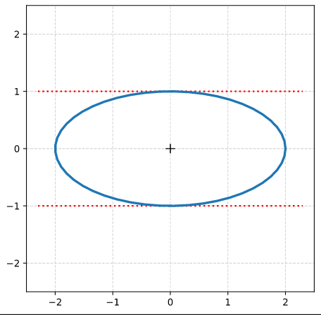
Step 0: Create 100 points a unit circle. Save the coordinates in Python lists (or Numpy arrays). Use Matplotlib’s plot(x,y)-function to plot the vectors.
Step 1: Create an axis-parallel ellipse with values for the axes ha = 2.0 and hb = 1.0 along the x- and the y-axis of the Cartesian coordinate system [CCS]. Do this by applying a diagonal scaling matrix Dσ1, σ2 (see the first post of this series).
Step 2: Rotate the ellipse bei π/3 (60 °). Do this by applying a rotation matrix Rπ/3 to the position vectors of your ellipse (with the help of Numpy). Alternatively, you can first create the matrices, perform a matrix multiplication and then apply the resulting matrix to the position vectors of your unit circle.
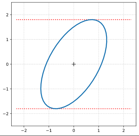
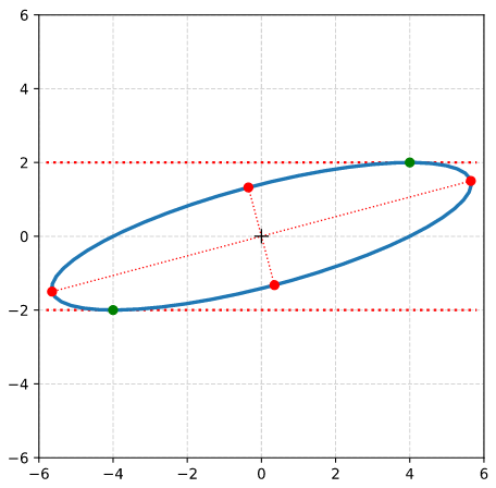
(The limiting lines have been calculated by the formulas given above.)
Step 3: Determine the coefficients of combined matrix AE = Rπ/3 ○ Dσ1, σ2
I got for the coefficients ( (a, b), (c, d) ) of AE :
A_ell =
[[ 1.         -0.8660254 ]
[ 1.73205081  0.5       ]]
Step 3: Determine the coefficients of the matrix Aq by the formulas given in the first post of this series. I got
A_q =
[[ 3.25       -1.29903811]
[-1.29903811  1.75      ]]
For δ I got:
delta = 4.0
which is consistent with the length-values of the principal axes.
Step 4: Determine values for the eigenvalues λ1 and λ2 from the Aq-coefficients by the formulas given in the first post. Also calculate them by using Numpy’s
eigenvalues, eigenvectors = numpy.linalg.eig(A_q). Theory tells us that these values should be exactly λ1 = 4 and λ1 = 1. I got
Eigenvalues from A_q: lambda_1 = 4. :: lambda_2 = 1.
Step 5: Determine the components of the normalized eigenvectors with the help of numpy.linalg.eig(A_q). I got:
Components of normalized eigenvectors by theoretical formulas from A_q coefficients:
ev_1_n :  -0.8660254037844386  :  0.5000000000000002
ev_2_n :  0.5000000000000001  :  0.8660254037844385

Eigenvectors from A_q via numpyy.linalg.eig():
ev_1_num :  0.8660254037844387  :  -0.5000000000000001
ev_2_num :  0.5000000000000001  :  0.8660254037844387
The deviation between ev_1_n and ev_1_num is just due to a difference by -1. This is correct as the eigenvectors are unique only up to a minus-sign in all components.
Step 6: Calculate the sinus of the rotation angle of our ellipse from Aq– and Aq-coefficients. The theoretical value is sin(2 π/3) = sin(2 pi/3) = 0.8660254037844387. I got:
sin(2. * rotation angle) of major axis of the ellipse against the CCS x-axis from A_E coefficients:
sin_2phi-A_E  =  0.8660254037844388

sin(2. * rotation angle) of major axis of the ellipse against the CCS x-axis from from eigenvectors of A_q:
sin_2phi-ev_A_q =  0.8660254037844387

sin(2. * rotation angle) of major axis of the ellipse against the CCS x-axis from A_q-coefficients:
sin_2phi-coeff-A_q =  0.8660254037844388
Perfect!
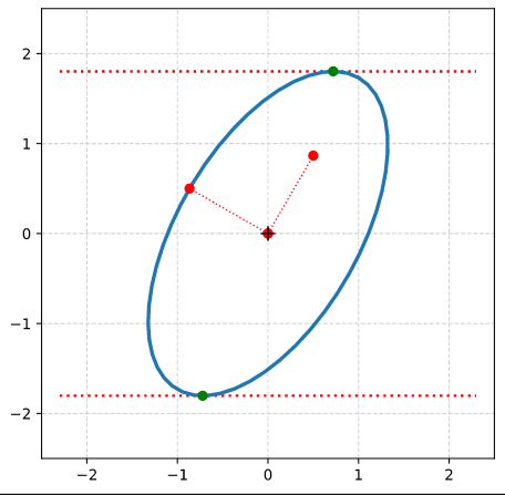
Step 7: Plot the end-points of the normalized eigenvectors of Aq:
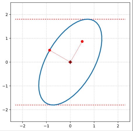
Note that in our example case the end-point of the eigenvector along the minor axis must be located exactly on the elliptic curve as the ellipses minor axes has a length of b=1!
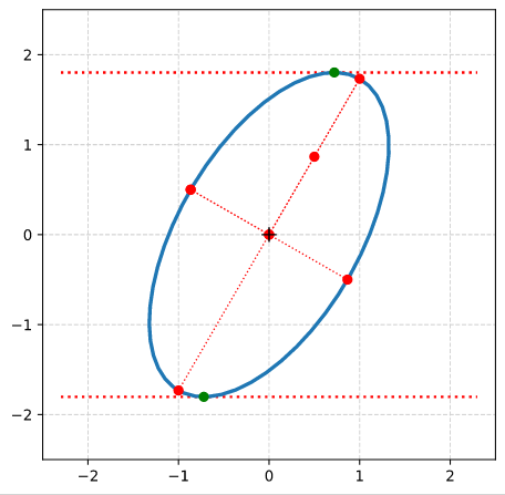
Step 8: Calculate the components of the vectors to data-points of the ellipse with maximal absolute ye-values from the Aq-coefficients given in the previous post. Plot these data-points (here in green color).
Step 9: Calculate the components of the vectors to data-points of the ellipse with maximal values of the radii with the help of the complex formulas presented in this post and plot these points in addition.
Conclusion
In this mini-series of posts we have performed some small mathematical exercises with respect to centered and rotated ellipses. We have calculated basic geometrical properties of such ellipses from the coefficients of matrices which define ellipses in algebraic form. Linear Algebra helped us to understand that the eigenvectors and eigenvalues of a symmetric matrix, whose coefficients stem from a quadratic equation (for a conic section), control both the orientation and the lengths of the ellipse’s axes completely.
This knowledge is useful in some Machine Learning [ML] context where elliptic data appear as projections of multivariate normal distributions. Multivariate Gaussian probability functions control properties of a lot of natural objects. Experience shows that certain types of neural networks may transform such data into multivariate normal distributions in latent spaces. An evaluation of the numerical data coming from such ML-experiments often delivers the coefficients of defining matrices for ellipses.
In my blog I now return to the study of with shearing operations applied to circles, spheres, ellipses and 3-dimensional ellipsoids. Later I will continue with the study of multivariate normal distributions in latent spaces of Autoencoders. For both of these topics the knowledge we have gathered regarding the matrices behind ellipses will help us a lot.