
I continue with my investigation of the z-point- and latent vector distribution which a convolutional Autoencoder [AE] creates in its latent space for CelebA images. Such images show human faces – and our objective is to find out whether we can force the AE’s Decoder to create human face images from artificially generated and statistically distributed z-points in the latent space. E.g. for creative tasks – without using a Variational Autoencoder.
The first posts of this series
Autoencoders and latent space fragmentation – I – Encoder, Decoder, latent space
Autoencoders and latent space fragmentation – II – number distributions of latent vector components
Autoencoders and latent space fragmentation – III – correlations of latent vector components
have revealed that the multi-dimensional volume region filled with z-points for CelebA images is rather small and has an ellipsoidal shape. The region is extended in the direction of a few main axes. Its center is located at some distance from the origin of the latent space. Its position is rather close to or within a hyper-volume of the latent space spanned by a few axes, only. The origin of the latent space is instead located close to the border of the bulk region of CelebA z-points.
We have also found out that artificially created z-points may miss the region of the CelebA z-points. In particular when we generate respective vectors under the assumption that the vector components are independent variables and can be filled with values obeying a constant probability distribution within a real value interval [-b, b]. See the second post for links to a study of the mathematical properties of such artificial vector distributions. We saw that the radii of the artificial vectors only match those of CelebA vectors if we choose 1.0 < b < 2.0. An optimal value appeared to be b = 1.5. This means that the created statistical vectors would have positions relatively close to the origin. We had hoped that such artificial vectors overlap at least in parts with the latent vector distribution for CelebA. Such an overlap may be required to get a reconstruction of images with clearly visible human faces.
In this post I, therefore, have a look at the surroundings of the latent space origin. We focus on projections of the neighboring z-points onto planes formed by selected latent vector components. We choose these components such that the border position of the origin with respect to the volume occupied by the bulk of CelebA z-points becomes clear. We afterward look at real and artificial z-points close to a slice of the multi-dimensional latent space volume. The vectors to the z-points in this slice fulfill the following condition: All components x_j, with the exception of two selected ones, have values x_j < 1.5. This will reduce projection effects with respect to the selected projection plane. The results will show us that many of the artificial z-points unfortunately fall into empty regions (voids). It is sufficient to show this for some selected coordinate pairs. The latent space of our AE has N=256 dimensions.
Position of the origin with respect to the CelebA z-point distribution
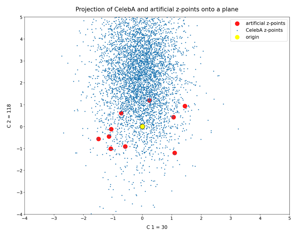
First I want to remind you of the border position of the latent space’s origin with respect to the bulk of the CelebA z-point-distribution. The following plots show again 5000 randomly selected z-points corresponding to latent vectors for CelebA images (blue points). The yellow point marks the origin of the latent space. The red dots correspond to 10 artificially created z-points for b = 1.5. The individual plots correspond to selected pairs of vector components and planes spanned by respective axes.
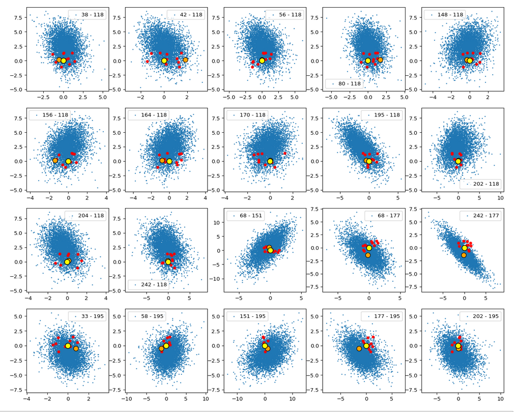
That the center of the distribution appears extremely densely populated is a bit due to the chosen diameter of the blue points. When interpreting these plots, please note: We are looking at orthogonal projections. Therefore we always have to take into account projection effects.
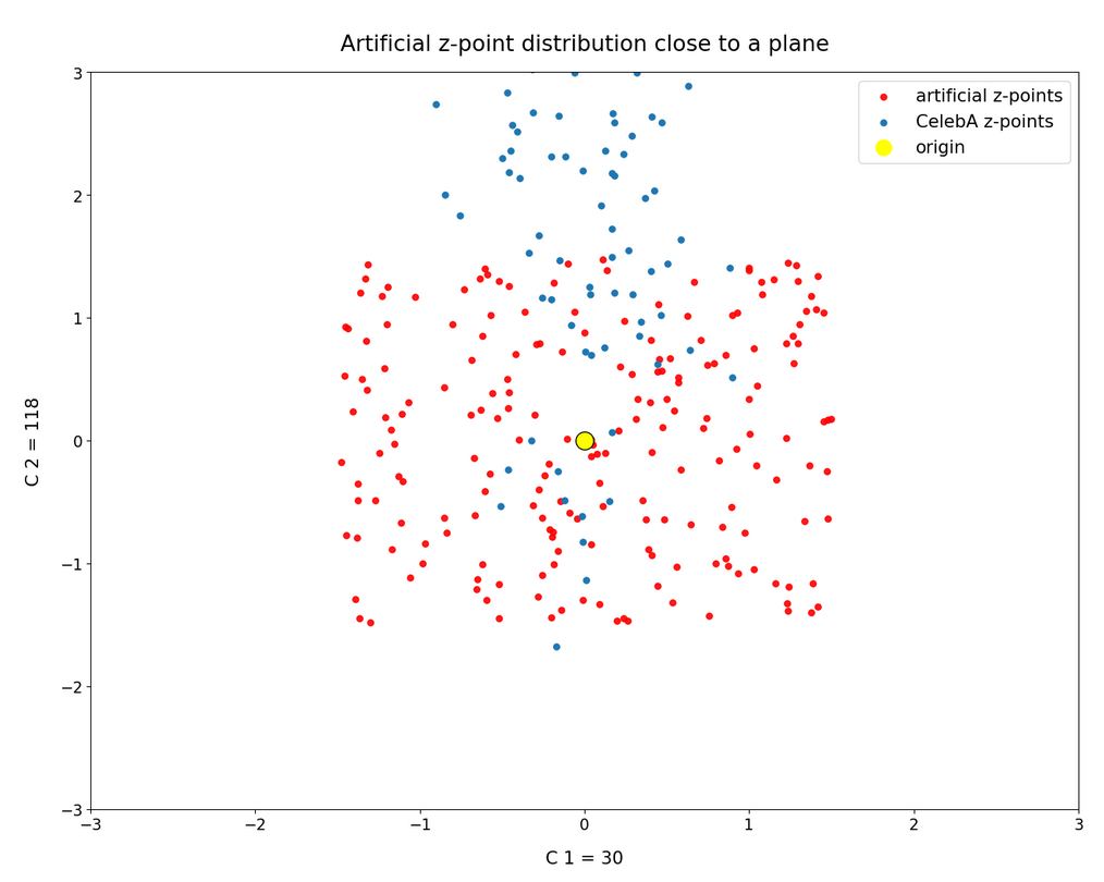
A closer look at the environment of the latent space’s origin
The following plot shows the environment of the origin with a higher resolution for our 5600 z-points. Despite the fact that this is a projection of many points onto the selected plane we get a first impression that CelebA z-point distribution is not really a homogeneous one – although being a relatively dense one around the center of the ellipsoidal bulk distribution.
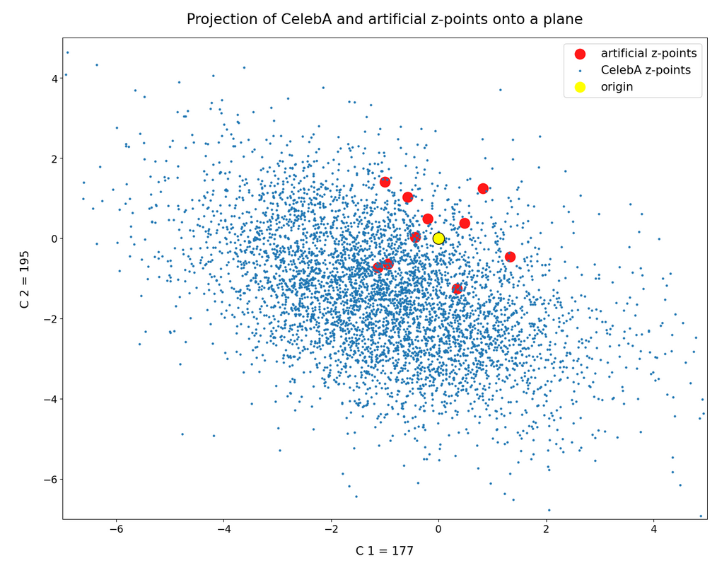
Some of our artificial z-points seem in both cases to mix with the CelebA z-points. Below I want to show that this is a projection effect, only.
The surroundings of the origin in a flat cuboid
In the second post of this series we had derived that a parameter b = 1.5 is optimal to get the right vector length of our artificial statistical vectors to match the length of the latent CelebA vectors. Therefore, I have reduced the amount of CelebA z-points by imposing the following conditions on the components x_j:
-1.5 ≤ x_j ≤ 1.5, for all j in [0, 256], with the exception of two selected values j = j1 or j = j2
I.e. we look at CelebA z-points close to the plane defined by the axes corresponding to our specially selected vector components x_j1 and x_j2. Thus we get rid of projection effects from any points outside the multi-dimensional slice. We only get projections from points inside our multi-dimensional slice, which contains the cube defined by a side-length -1.5 ≤ x_j ≤ +1.5 around the origin. Our statistically generated vectors have end-points inside this multi-dimensional cube. The result is:

Ooops, only two out of our 5000 CelebA points are present in the slice region, which I also have populated with 200 artificial z-points. So, clearly this is not a region which the AE’s Encoder fills densely for CelebA images.
Even for 80,000 CelebA z-points the situation does not improve so much. Only 56 latent CelebA vectors point to our region.
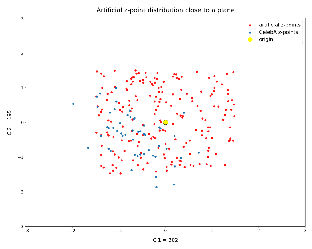
Most of the artificially created z-points (in red) thus come to fall into empty volume regions – regions not used by CelebA z-points. This already diminishes our chances to reconstruct reasonable human face images by our artificial distribution of latent vectors.
Situation for a second and a third plane
Can we reproduce this also for other component pairs? Yes, indeed, e.g. for the pair (177, 242):
For 5000 CelebA z-points:

Only one out of 5000 CelebA vectors points to the relevant slice:
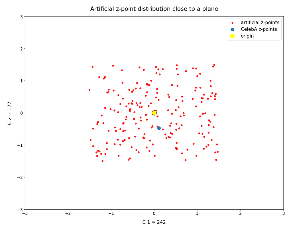
For 80,000 images 39 regular CelebA z-points survive, only. I skip the respective image.
Vector components (30, 118)
Another interesting pair of components and respective coordinate axes is (30, 118):
And for our slice we get:
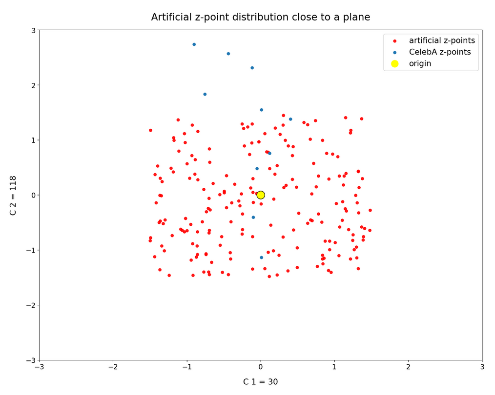
From 80,000 points only around 70 are located in our slice of the multidimensional space:
Vector components (118, 156)
For the pair (118, 156) the respective plots are:

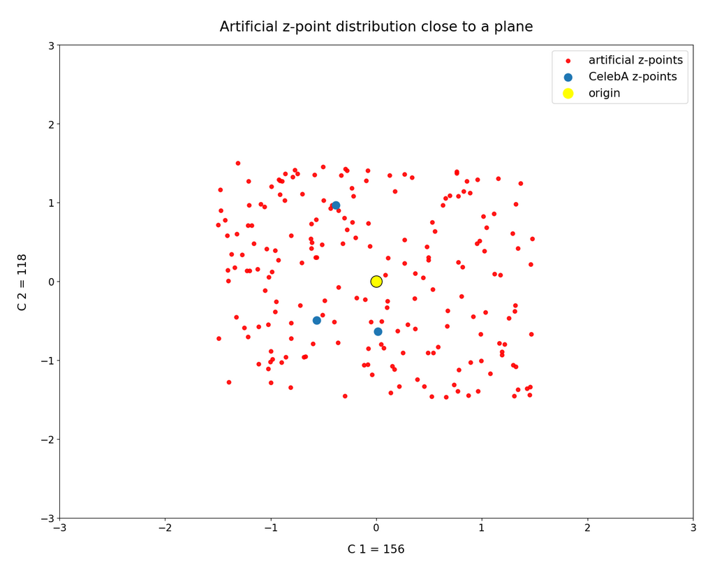

We see some overlaps between the artificially created points and the CelebA z-points. However, you should keep in mind that the probability that an artificial point falls into a void in the multi-dimensional space gets bigger with every individual component value putting the point outside the CelebA bulk region. And: Our “overlaps” are still the result of a (significantly reduced) projection effect. Furthermore, the plots do not distinguish the components of an individual point from those of other points. If one component shows an overlap with CelebA points, another component for the same point may not. And one component is enough to determine a position outside the bulk.
Radii of the artificially created z-points
When rating probabilities of our artificially created z-points to hit a region populated by CelebA z-points you should also remember that our artificially created points fall into a rather narrow spherical shell for so many dimensions as our latent space has. See the second post of this series for this phenomenon.
Conclusion
What have we learned? The second post in this series gave us hope that at least some of the artificially created z-points (based on independent component values taken with a constant probability from a common value interval) would get a position within the confined region populated by the real CelebA z-points. A closer look, however, showed us that the origin of the latent space resides within a border-region of the ellipsoidal bulk of the multi-dimensional CelebA z-point distribution. Only very few CelebA z-points are found in this border region and within slices close to selected coordinate planes.
What does this mean? The chances that most of the artificially created z-points for b = 1.5 will fall into a void not used by the AE’s Decoder for CelebA images is much bigger than we originally may have thought. In addition our statistical points only populate a spherical shell within a multi-dimensional cube around the origin of the latent space with a side length of 2b. Even if we compensate this effect by generating vectors for different b-values we do not gain much. This raises the fundamental question whether a method that generates statistical z-points via independent component values is a reasonable choice for our objective to reconstruct human face images.
In the next post
I will show that the results of such reconstruction efforts are indeed frustrating. As a consequence I will discuss how we could simply adjust our generating method to the real distribution of latent vectors for CelebA images.