A simple CNN for the MNIST dataset – VII – outline of steps to visualize image patterns which trigger filter maps

During my present article series on a simple CNN we have seen how we set up and train such an artificial neural network with the help of Keras.

A simple CNN for the MNIST dataset – VI – classification by activation patterns and the role of the CNN’s MLP part
A simple CNN for the MNIST dataset – V – about the difference of activation patterns and features
A simple CNN for the MNIST dataset – IV – Visualizing the activation output of convolutional layers and maps
A simple CNN for the MNIST dataset – III – inclusion of a learning-rate scheduler, momentum and a L2-regularizer
A simple CNN for the MNIST datasets – II – building the CNN with Keras and a first test
A simple CNN for the MNIST datasets – I – CNN basics

Lately we managed to visualize the activations of the maps which constitute the convolutional layers of a CNN {Conv layer]. A Conv layer in a CNN basically is a collection of maps. The chain of convolutions produces characteristic patterns across the low dimensional maps of the last (i.e. the deepest) convolutional layer – in our case of the 3rd layer “Conv2D_3”. Such patterns obviously improve the classification of images with respect to their contents significantly in comparison to pure MLPs. I called a node activation pattern within or across CNN maps a FCP (see the fifth article of this series).

The map activations of the last convolutional layer are actually evaluated by a MLP, whose dense layer we embedded in our CNN. In the last article we therefore also visualized the activation values of the nodes within the first dense MLP-layer. We got some indications that map activation patterns, i.e. FCPs, for different image classes indeed create significantly different patterns within the MLP – even when the human eye does not directly see the decisive difference in the FCPs in problematic and confusing cases of input images.

In so far the effect of the transformation cascade in the convolutional parts of a CNN is somewhat comparable to the positive effect of a cluster analysis of MNIST images ahead of a MLP classification. Both approaches correspond to a projection of the input data into lower dimensional representation spaces and provide clearer classification patterns to the MLP. However, convolutions do a far better job to produce distinguished patterns for a class of images than a simple cluster analysis. The assumed reason is that chained convolutions somehow identify characteristic patterns within the input images themselves.

Is there a relation between a FCP and a a pattern in the pixel distribution of the input image?

But so far, we did not get any clear idea about the relation of FCP-patterns with pixel patterns in the original image. In other words: We have no clue about what different maps react to in terms of characteristic patterns in the input images. Actually, we do not even have a proof that a specific map – or more precisely the activation of a specific map – is triggered by some kind of distinct pattern in the value distribution for the original image pixels.

I call an original pattern to which a CNN map strongly reacts to an OIP; an OIP thus represents a certain geometrical pixel constellation in the input image which activates neurons in a specific map very strongly. Not more, not less. Note that an OIP therefore represents an idealized pixel constellation – a pattern which at best is free of any disturbances which might reduce the activation of a specific map. Can we construct an image with just the required OIP pixel constellation to trigger a map optimally? Yes, we can – at least approximately.

In the present article I shall outline the required steps which will enable us to visualize OIPs later on. In my opinion this is an important step to understand the abilities of CNNs a bit better. In particular it helps to clarify whether and in how far the term “feature detection” is appropriate. In our case we look out for primitive patterns in the multitude of MNIST images of handwritten digits. Handwritten digits are interesting objects regarding basic patterns – especially as we humans have some very clear abstract and constructive concepts in mind when we speak about basic primitive elements of digit notations – namely line and bow segments which get arranged in specific ways to denote a digit.

At the end of this article we shall have a first look at some OIP patterns which trigger a few chosen individual maps of the third convolutional layer of our CNN. In the next article I shall explain required basic code elements to create such OIP pictures. Subsequent articles will refine and extend our methods towards a more systematic analysis.

Questions and objectives

We shall try to answer a series of questions to approach the subject of OIPs and features:

  • How can Keras help us to find and visualize an OIP which provokes a maximum average reaction of a map?
  • How well is the “maximum” defined with respect to input data of our visualization method?
  • Do we recognize sub-patterns in such OIPs?
  • How do the OIPs – if there are any – reflect a translational invariance of complex, composed patterns?
  • What does a maximum activation of an individual node of a map mean in terms of an input pattern?

What do I mean by “maximum average reaction“? A specific map of a CNN corresponds to a 2-dim array of “neurons” whose activation functions produce some output. The basic idea is that we want to achieve a maximum average value of this output by systematically optimizing initially random input image data until, hopefully, a pattern emerges.

Basic strategy to visualize an OIP pattern

In a way we shall try to create order out of chaos: We want to systematically modify an initial random distribution of pixel values until we reach a maximum activation of the chosen map. We already know how to systematically approach a minimum of a function depending on a multidimensional arrangement of parameters. We apply the “gradient descent” method to a hyperplane created by a suitable loss-function. Considering the basic principles of “gradient descent” we may safely assume that a slightly modified gradient guided approach will also work for maxima. This in turn means:

We must define a map-specific “loss” function which approaches a maximum value for optimum node activation. A suitable simple function could be a sum or average increasing with the activation values of the map’s nodes. So, in contrast to classification tasks we will have to use a “gradient ascent” method- The basic idea and a respective simple technical method is e.g. described in the book of F. Chollet (Deep Learning mit Python und Keras”, 2018, mitp Verlag; I only have the German book version, but the original is easy to find).

But what is varied in such an optimization model? Certainly not the weights of the already trained CNN! The variation happens with respect to the input data – the initial pixel values of the input image are corrected by the gradient values of the loss function.

Next question: What do we choose as a starting point of the optimization process? Answer: Some kind of random distribution of pixel values. The basic hope is that a gradient ascent method searching for a maximum of a loss function would also “converge“.

Well, here began my first problem: Converge in relation to what exactly? With respect to exactly one input input image or to multiple input images with different initial statistical distributions of pixel data? With fluctuations defined on different wavelength levels? (Physicists and mathematicians automatically think of a Fourier transformation at this point 🙂 ). This corresponds to the question whether a maximum found for a certain input image really is a global maximum. Actually, we shall see that the meaning of convergence is a bit fuzzy in our present context and not as well defined as in the case of a CNN-training.

To discuss fluctuations in statistical patterns at different wavelength is not so far-fetched as it may seem: Already the basic idea that a map reacts to a structured and maybe sub-structured OIP indicates that pixel correlations or variations on different length scales might play a role in triggering a map. We shall see that some maps do not react to certain “random” patterns at all. And do not forget that pooling operations induce the analysis of long range patterns by subsequent convolutional filters. The relevant wavelength is roughly doubled by each of our pooling operations! So, filters at deep convolutional layers may exclude patterns which do not show some long range characteristics.

The simplified approach discussed by Chollet assumes statistical variations on the small length scale of neighboring pixels; he picks a random value for each and every pixel of his initial input images without any long range correlations. For many maps this approach will work reasonably well and will give us a basic idea about the average pattern or, if you absolutely want to use the expression, “feature”, which a CNN-map reacts to. But being able to vary the length scale of pixel values of input images will help us to find patterns for sensitive maps, too.

We may not be able to interpret a specific activation pattern within a map; but to see what a map on average and what a single node of a map reacts to certainly would mean some progress in understanding the relation between OIPs and FCPs.

An example

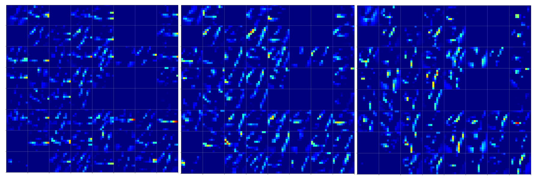
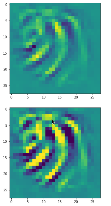
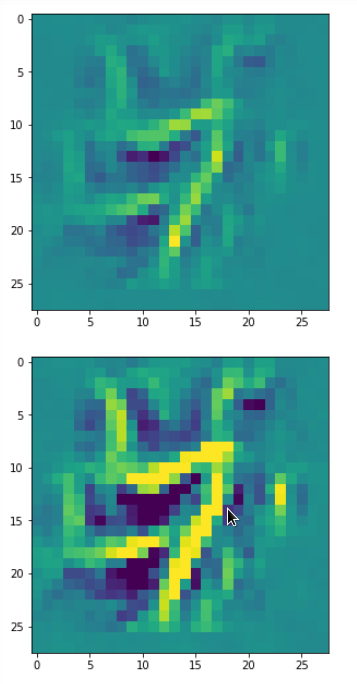
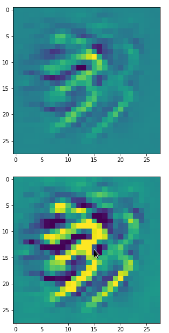
The question what an OIP is depends on the scales you look at and also where an OIP appears within a real image. To confuse you a bit: Look at he following OIP-picture which triggered a certain map strongly:

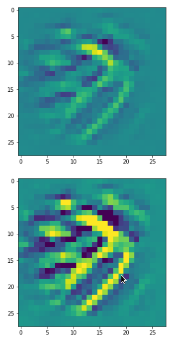
The upper image was prepared with a plain color map, the lower with some contrast enhancement. I use this two-fold representation also later for other OIP-pictures.

Actually, it is not so clear what elementary pattern our map reacts to. Two parallel line segments with a third one crossing perpendicular at the upper end of the parallel segments?

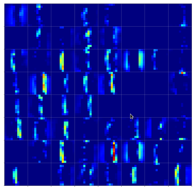
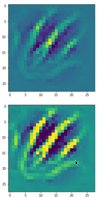
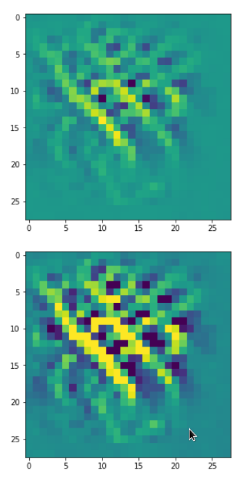
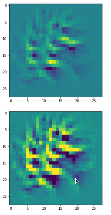
One reason for being uncertain is that some patterns on a scale of lets say a fourth of the original image may appear at different locations in original images of the same class. If a network really learned about such reappearance of patterns the result for an optimum OIP may be a superposition of multiple elementary patterns at different locations. Look at the next two OIP pictures for the very same map – these patterns emerged from a slightly different statistical variation of the input pixel values:

Now, we recognize some elementary structures much better – namely a combination of bows with slightly different curvatures and elongations. Certainly useful to detect “3” digits, but parts of “2”s, too!

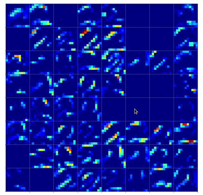
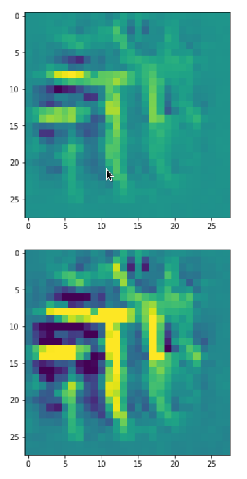
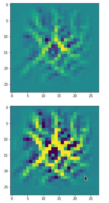
A different version of another map is given here:

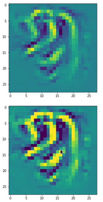
Due to the large scale structure over the full height of the input this map is much better suited to detect “9”s at different places.

You see that multiple filters on different spatial resolution levels have to work together in this case to reflect one bow – and the bows elongation gets longer with their position to the right. It seems that the CNN has learned that bow elements with the given orientation on the left side of original images are smaller and have a different degree of curvature than to the right of a MNIST input image. So what is the OIP or what is the “feature” here? The superposition of multiple translationally shifted and differently elongated bows? Or just one bow?

Unexpected technical hurdles

I was a bit surprised that I met some technical difficulties along my personal way to answer the questions posed above. The first point is that only a few text book authors seem to discuss the question at all; F. Chollet being the remarkable exception and most authors in the field, also of articles on the Internet, refer to his ideas and methods. I find this fact interesting as many authors of introductory books on ANNs just talk about “features” and make strong claims about what “features” are in terms of entities and their detection by CNNs – but they do not provide any code to verify the almost magic “identification” of conceptual entities as “eyes”, “feathers”, “lips”, etc..

Then there are articles of interested guys, which appear at specialized web sites, as e.g. the really read-worthy contribution of the physicist F. Graetz: https://towardsdatascience.com/how-to-visualize-convolutional-features-in-40-lines-of-code-70b7d87b0030 on “towardsdatascience.com”. His color images of “features” within CIFAR images are impressive; you really should have a look at them.

But he as other authors usually take pre-trained nets like VGG16 and special datasets as CIFAR with images of much higher resolution than MNIST images. But I wanted to apply similar methods upon my own simple CNN and MNIST data. Although an analysis of OIPs of MNIST images will certainly not produce such nice high resolution color pictures as the ones of Graetz, it might be easier to extract and understand some basic principles out of numerical experiments.

Unfortunately, I found that I could not just follow and copy code snippets of F. Chollet. Partially this had to do with necessary changes Tensorflow 2 enforced in comparison to TF1 which was used by F. Chollet. Another problem was due to standardized MNIST images my own CNN was trained on. Disregarding the point of standardization during programming prevented convergence during the identification of OIPs. Another problem occurred with short range random value variations for the input image pixels as a starting point. Choosing independent random values for individual pixels suppresses long range variations; this in turn often leads to zero gradients for averaged artificial “costs” of maps at high layer levels.

A better suitable variant of Chollet’s code with respect to TF 2 was published by a guy named Mohamed at “https://www.kaggle.com/questions-and-answers/121398“. I try to interpret his line of thinking and coding in my forthcoming articles – so all credit belongs to him and F. Chollet. Nevertheless, as said, I still had to modify their code elements to take into account special aspects of my own trained CNN.

Basic outline for later coding

We saw already in previous articles that we can build new models with Keras and TensorFlow 2 [TF2] which connect some input layer with the output of an intermediate layer of an already defined CNN- or MLP-model. TF2 analyses the respective dependencies and allows for a forward propagation of input tensors to get the activation values ( i.e. the output values of the activation function) at the intermediate layer of the original model – which now plays the role of an output layer in the new (sub-) model.

However, TF2 can do even more for us: We can define a specific cost function, which depends on the output tensor values of our derived sub-model. TF2 will also (automatically) provide gradient values for this freshly defined loss function with respect to input values which we want to vary.

The basic steps to construct images which trigger certain maps optimally is the following:

  • We construct an initial input image filled with random noise. In the case of MNIST this input image would consist of input values on a 1-dim gray scale. We standardize the input image data as our CNN has been trained for such images.
  • We build a new model based on the layer structure of our original (trained) CNN-model: The new model connects the input-image-tensor at the input layer of the CNN with the output generated of a specific feature map at some intermediate layer after the forward propagation of the input data.
  • We define a new loss function which should show a maximum value for the map output – depending of course on optimized input image data for the chosen specific map.
  • We define a suitable (stochastic) gradient ascent method to approach the aspired maximum for corrected input image data.
  • We “inform” TF2 about the gradient’s dependencies on certain varying variables to give us proper gradient values. This step is of major importance in Tensorflow environments with activated “eager execution”. (In contrast to TF1 “eager execution” is the standard setting for TF2.)
  • We scale (= normalize) the gradient values to avoid too extreme corrections of the input data.
  • We take into account a standardization of the corrected input image data. This will support the overall convergence of our approach.
  • We in addition apply some tricks to avoid a over-exaggeration of small scale components (= high frequency components in the sense of a Fourier transform) in the input image data.

Especially the last point was new to me before I read the code of Mohamed at Kaggle. E.g. F. Chollet does not discuss this point in his book. But it is a very clever thought that one should care about low and high frequency contributions in patterns which trigger maps at deep convolutional layers. Whereas Mohamed discusses the aspect that high frequency components may guide the optimization process into overall side maxima during gradient ascent, I would in addition say that not offering long range variations already in the statistical input data may lead to a total non-activation of some maps. Actually, this maybe is an underestimated crucial point in the hunt for patterns which trigger maps – especially when we deal with low resolution input images.

Eager mode requirements

Keras originally provided a function “gradients()” which worked with TF1 graphs and non-eager execution mode. However, T2 executes code in eager mode automatically and therefore we have to use special functions to control gradients and their dependencies on changing variables (see for a description of “eager execution” https://www.tensorflow.org/guide/eager?hl=en ).

Among other things: TF2 provides a special function to “watch” variables whose variations have an impact on loss functions and gradient values with respect to a defined (new) model. (An internal analysis by TF2 of the impact of such variations is of course possible because our new sub-model is based on an already given layer structures of the original CNN-model.)

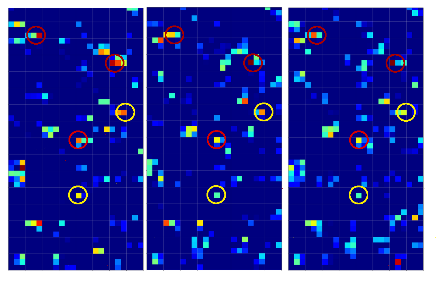
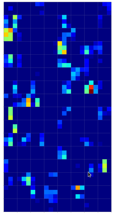
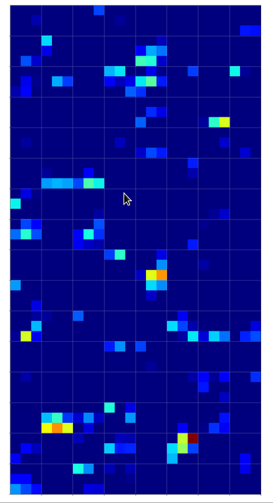
Visualization of some OIP-patterns in MNIST images as appetizers

Enough for today. To raise your appetite for more I present some images of OIPs. I only show patterns triggering maps on the third Conv-layer.

There are simple patterns:

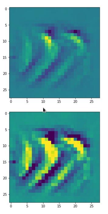
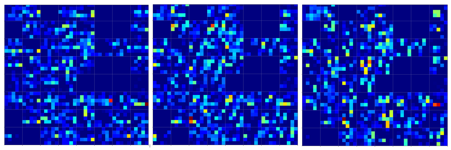
But there are also more complex ones:

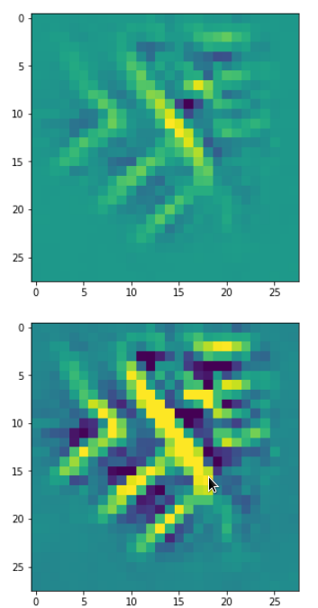
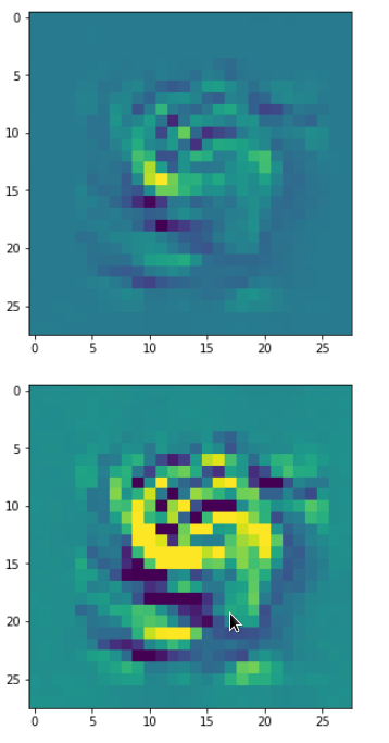
A closer look shows that the complexity results from translations and rotations of elementary patterns.

Conclusion

In this article we have outlined steps to build a program which allows the search for OIPs. The reader has noticed that I try to avoid the term “features”. First images of OIPs show that such patterns may appear a bit different in different parts of original input images. The maps of a CNN seem to take care of this. This is possible, only, if and when pixel correlations are evaluated over many input images and if thereby variations on larger spatial scales are taken into account. Then we also have images which show unique patterns in specific image regions – i.e. a large scale pattern without much translational invariance.

We shall look in more detail at such points as soon as we have built suitable Python functions. See the next post

A simple CNN for the MNIST dataset – VIII – filters and features – Python code to visualize patterns which activate a map strongly


A simple CNN for the MNIST dataset – VI – classification by activation patterns and the role of the CNN’s MLP part

I continue with my series on a simple CNN used upon the MNIST dataset.

A simple CNN for the MNIST dataset – V – about the difference of activation patterns and features
A simple CNN for the MNIST dataset – IV – Visualizing the activation output of convolutional layers and maps
A simple CNN for the MNIST dataset – III – inclusion of a learning-rate scheduler, momentum and a L2-regularizer
A simple CNN for the MNIST datasets – II – building the CNN with Keras and a first test
A simple CNN for the MNIST datasets – I – CNN basics

In the last article I discussed the following points:

  • The series of convolutional transformations, which a CNN applies to its input, eventually leads to abstract representations in low dimensional parameter spaces, called maps. In the case of our CNN we got 128 (3×3)-maps at the last convolutional layer. 3×3 indeed means a very low resolution.
  • We saw that the transformations would NOT produce results on the eventual maps which could be interpreted in the sense of figurative elements of depicted numbers, such as straight lines, circles or bows. Instead, due to pooling layers, lines and curved line elements obviously experience a fast dissolution during propagation through the various Conv layers. Whilst the first Conv layer still gives fair representations of e.g. a “4”, line-like structures get already unclear at the second Conv layer and more or less disappear at the maps of the last convolutional layer.
  • This does not mean that a map on a deep convolutional layer does not react to some specific pattern within the pixel data of an input image. We called such patterns OIPs in last article and we were careful to describe them as geometrical correlations of pixels – and not conceptual entities. The sequence of convolutions which makes up a map on a deep convolutional layer corresponds to a specific combination of filters applied to the image data. This led us to the the theoretical idea that a map may indeed select a specific OIP in an input image and indicate the existence of such a OIP pattern by some activation pattern of the “neurons” within the map. However, we have no clue at the moment what such OIPs may look like and whether they correspond to conceptual entities which other authors usually call “features”.
  • We saw that the common elements of the maps of multiple images of a handwritten “4” correspond to point-like activations within specific low dimensional maps on the output side of the last convolutional layer.
  • The activations seem to form abstract patterns across the maps of the last convolutional layer. These patterns, which we called FCPs, seem to support classification decisions, which the MLP-part of the CNN has to make.

So, at our present level of the analysis of a CNN, we cannot talk in a well founded way about “features” in the sense of conceptual entities. We got, however, the impression that eventual abstractions of some patterns which are present in MNIST images of different digits lead to FCP patterns across maps which allow for a classification of the images (with respect to the represented digits). We identified at least some common elements across the eventual maps of 3 different images of handwritten “4”s.

But it is really this simple? Can we by just looking for visible patterns in the activation output of the last convolutional layer already discriminate between different digits?

In this article I want to show that this is NOT the case. To demonstrate this we shall look at the image of a “4” which could also be almost classified to represent a “9”. We shall see

  • that the detection of clear unique patterns becomes really difficult when we look at the representations of “4”s which almost resemble a “9” – at least from a human point of view;
  • that directly visible patterns at the last convolutional layer may not contain sufficiently clear information for a classification;
  • that the MLP part of our CNN nevertheless detects patterns after a linear transformation – i.e. after a linear combination of the outputs of the last Conv layer – which are not directly evident for human eyes. These “hidden” patterns do, however, allow for a rather solid classification.

What have “4”s in common after three convolutional transformations?

As in the last article I took three clear “4” images

and compared the activation output after three convolutional transformations – i.e. at the output side of the last Conv layer which we named “Conv2D_3”:

The red circles indicate common points in the resulting 128 maps which we do not find in representations of three clear “9”s (see below). The yellow circles indicate common patterns which, however, appear in some representations of a “9”.

What have “9”s in common after three convolutional transformations?

Now let us look at the same for three clear “9”s:


A comparison gives the following common features of “9”s on the third Conv2D layer:

We again get the impression that enough unique features seem to exist on the maps for “4”s and “9”s, respectively, to distinguish between images of these numbers. But is it really so simple?

Intermezzo: Some useful steps to reproduce results

You certainly do not want to perform a training all the time when you want to analyze predictions at certain layers for some selected MNIST images. And you may also need the same “X_train”, “X_test” sets to identify one and the same image by a defined number. Remember: In the Python code which I presented in a previous article for the setup for the data samples no unique number would be given due to initial shuffling.

Thus, you may need to perform a training run and then save the model as well as your X_train, y_train and X_test, y_test datasets. Note that we have transformed the data already in a reasonable tensor form which Keras expects. We also had already used one-hot-labels. The transformed sets were called “train_imgs”, “test_imgs”, “train_labels”, “test_labels”, “y_train”, “y_test”

The following code saves the model (here “cnn”) at the end of a training and loads it again:

# save a full model 
cnn.save('cnn.h5')

#load a full model  
cnnx = models.load_model('cnn.h5')        

On a Linux system the default path is typically that one where you keep your Jupyter notebooks.

The following statements save the sets of tensor-like image data in Numpy compatible data (binary) structures:

# Save the data

from numpy import save
save('train_imgs.npy', train_imgs) 
save('test_imgs.npy', test_imgs) 
save('train_labels.npy', train_labels) 
save('test_labels.npy', test_labels) 
save('y_train.npy', y_train) 
save('y_test.npy', y_test) 

We reload the data by

# Load train, test image data (in tensor form) 

from numpy import load
train_imgs   = load('train_imgs.npy')
test_imgs    = load('test_imgs.npy')
train_labels = load('train_labels.npy')
test_labels  = load('test_labels.npy')
y_train      = load('y_train.npy')
y_test       = load('y_test.npy')

Be careful to save only once – and not to set up and save your training and test data again in a pure analysis session! I recommend to use different notebooks for training and later analysis. If you put all your code in just one notebook you may accidentally run Jupyter cells again, which you do not want to run during analysis sessions.

What happens for unclear representations/images of a “4”?

When we trained a pure MLP on the MNIST dataset we had a look at the confusion matrix:
A simple Python program for an ANN to cover the MNIST dataset – XI – confusion matrix.
We saw that the MLP e.g. confused “5”s with “9s”, “9”s with “4”s, “2”s with “7”s, “8”s with “5”s – and vice versa. We got the highest confusion numbers for the misjudgement of badly written “4”s and “9”s.

Let us look at a regular 4 and two “4”s which with some good will could also be interpreted as representations of a “9”; the first one has a closed upper area – and there are indeed some representations of “9”s in the MNIST dataset which look similar. The second “4” in my view is even closer to a “9”:


Now, if we wanted to look out for the previously discussed “unique” features of “4”s and “9s” we would get a bit lost:

The first image is for a clear “4”. The last two are the abstractions for our two newly chosen unclear “4”s in the order given above.

You see: Many of our seemingly “unique features” for a “4” on the third Conv-level are no longer or not fully present for our second “4”; so we would be rather insecure if we had to judge the abstraction as a viable pattern for a “4”. We would expect that this “human” uncertainty also shows up in a probability distribution at the output layer of our CNN.

But, our CNN (including its MLP-part) has no doubt about the classification of the last sample as a “4”. We just look at the prediction output of our model:

# Predict for a single image 
# ****************************
num_img = 1302
ay_sgl_img = test_imgs[num_img:num_img+1]
print(ay_sgl_img.shape)
# load last cell for the next statement to work 
#prob = cnn_pred.predict_proba(ay_sgl_img, batch_size=1)
#print(prob) 
prob1 = cnn_pred.predict(ay_sgl_img, batch_size=1)
print(prob1) 

[[3.61540742e-07 1.04205284e-07 1.69877489e-06 1.15337198e-08
  9.35641170e-01 3.53500056e-08 1.29525617e-07 2.28584581e-03
  2.59062881e-06 6.20680153e-02]]

93.5% probability for a “4”! A very clear discrimination! How can that be, given the – at first sight – seemingly unclear pattern situation at the third activation layer for our strange 4?

The MLP-part of the CNN “sees” things we humans do not see directly

We shall not forget that the MLP-part of the CNN plays an important role in our game. It reduces the information of the last 128 maps (3x3x128 = 1152) values down to 100 node values with the help of 115200 distinguished weights for related connections. This means there is a lot of fine-tuned information extraction and information compactification going on at the border of the CNN’s MLP part – a transformation step which is too complex to grasp directly.

It is the transformation of all the 128x3x3-map-data into all 100 nodes via a linear combination which makes things difficult to understand. 115200 optimized weights leave enough degrees of freedom to detect combined patterns in the activation data which are more complex and less obvious than the point-like structures we encircled in the images of the maps.

So, it is interesting to visualize and see how the MLP part of our CNN reacts to the activations of the last convolutional layers. Maybe we find some more intriguing patterns there, which discriminate “4”s from “9”s and explain the rather clear probability evaluation.

Visualization of the output of the dense layers of the CNN’s MLP-part

We need to modify some parts of our code for creating images of the activation outputs of convolutional layers to be able to produce equally reasonable images for the output of the dense MLP layers, too. These modifications are simple. We distinguish between the types of layers by their names: When the name contains “dense” we execute a slightly different code. The changes affect just the function “img_grid_of_layer_activation()” previously discussed as the contents of a Jupyter “cell 9“:

  
# Function to plot the activations of a layer 
# --------------------------
-----------------
# Adaption of a method originally designed by F.Chollet 

def img_grid_of_layer_activation(d_img_sets, model_fname='cnn.h5', layer_name='', img_set="test_imgs", num_img=8, 
                                 scale_img_vals=False):
    '''
    Input parameter: 
    -----------------
    d_img_sets: dictionary with available img_sets, which contain img tensors (presently: train_imgs, test_imgs)  
    model_fname: Name of the file containing the models data 
    layer_name: name of the layer for which we plot the activation; the name must be known to the Keras model (string) 
    image_set: The set of images we pick a specific image from (string)
    num_img: The sample number of the image in the chosen set (integer) 
    scale_img_vals: False: Do NOT scale (standardize) and clip (!) the pixel values. True: Standardize the values. (Boolean)
        
    Hints: 
    -----------------
    We assume quadratic images - in case of dense layers we assume a size of 1 
    '''
    
    # Load a model 
    cnnx = models.load_model(model_fname)
    
    # get the output of a certain named layer - this includes all maps
    # https://keras.io/getting_started/faq/#how-can-i-obtain-the-output-of-an-intermediate-layer-feature-extraction
    cnnx_layer_output = cnnx.get_layer(layer_name).output

    # build a new model for input "cnnx.input" and output "output_of_layer"
    # ~~~~~~~~~~~~~~~~~
    # Keras knows the required connections and intermediat layers from its tensorflow graphs - otherwise we get an error 
    # The new model can make predictions for a suitable input in the required tensor form   
    mod_lay = models.Model(inputs=cnnx.input, outputs=cnnx_layer_output)
    
    # Pick the input image from a set of respective tensors 
    if img_set not in d_img_sets:
        print("img set " + img_set + " is not known!")
        sys.exit()
    # slicing to get te right tensor 
    ay_img = d_img_sets[img_set][num_img:(num_img+1)]
    
    # Use the tensor data as input for a prediction of model "mod_lay" 
    lay_activation = mod_lay.predict(ay_img) 
    print("shape of layer " + layer_name + " : ", lay_activation.shape )
    
    # number of maps of the selected layer 
    n_maps   = lay_activation.shape[-1]
    print("n_maps = ", n_maps)

    # size of an image - we assume quadratic images 
    # in the case  of "dense" layers we assume that the img size is just 1 (1 node)    
    if "dense" in layer_name:
        img_size = 1
    else: 
        img_size = lay_activation.shape[1]
    print("img_size = ", img_size)

    # Only for testing: plot an image for a selected  
    # map_nr = 1 
    #plt.matshow(lay_activation[0,:,:,map_nr], cmap='viridis')

    # We work with a grid of images for all maps  
    # ~~~~~~~~~~~~~~~----------------------------
    # the grid is build top-down (!) with num_cols and num_rows
    # dimensions for the grid 
    num_imgs_per_row = 8 
    num_cols = num_imgs_per_row
    num_rows = n_maps // num_imgs_per_row
    #print("img_size = ", img_size, " num_cols = ", num_cols, " num_rows = ", num_rows)

    # grid 
    dim_hor = num_imgs_per_row * img_size
    dim_ver = num_rows * img_size
    img_grid = np.zeros( (dim_ver, dim_hor) )   # horizontal, vertical matrix  
    print("shape of img grid = ", img_grid.shape)

    # double loop to fill the grid 
    n = 0
    for row in range(num_rows):
        for col in range(num_cols):
            n += 1
            #print("n = ", n, "row = ", row, " col = ", col)
            # in case of a dense layer the shape of the tensor like output 
            # is different in comparison to Conv2D layers  
            if "dense" in layer_name:
                present_img = lay_activation[ :, row*num_imgs_per_row + col]
            else: 
             
   present_img = lay_activation[0, :, :, row*num_imgs_per_row + col]
            
            # standardization and clipping of the img data  
            if scale_img_vals:
                present_img -= present_img.mean()
                if present_img.std() != 0.0: # standard deviation
                    present_img /= present_img.std()
                    #present_img /= (present_img.std() +1.e-8)
                    present_img *= 64
                    present_img += 128
                present_img = np.clip(present_img, 0, 255).astype('uint8') # limit values to 255

            # place the img-data at the right space and position in the grid 
            # ~~~~~~~~~~~~~~~~~~~~~~~~~~~~~~~~~~~~~~~~~~~~~~~~~~~~~~~~~~~~~~
            # the following is only used if we had reversed vertical direction by accident  
            #img_grid[row*img_size:(row+1)*(img_size), col*img_size:(col+1)*(img_size)] = np.flip(present_img, 0)
            img_grid[row*img_size:(row+1)*(img_size), col*img_size:(col+1)*(img_size)] = present_img
 
    return img_grid, img_size, dim_hor, dim_ver 


You certainly detect the two small changes in comparison to the code for Jupyter cell 9 of the article
A simple CNN for the MNIST dataset – IV – Visualizing the output of convolutional layers and maps.

However, there remains one open question: We were too lazy in the coding discussed in previous articles to create our own names names for the dense layers. This is, however, no major problem: Keras creates its own names – if we do not define our own layer names when constructing a CNN model. Where do we get these default names from? Well, from the model’s summary:

cnn_pred.summary()

Model: "sequential_7"
_________________________________________________________________
Layer (type)                 Output Shape              Param #   
=================================================================
Conv2D_1 (Conv2D)            (None, 26, 26, 32)        320       
_________________________________________________________________
Max_Pool_1 (MaxPooling2D)    (None, 13, 13, 32)        0         
_________________________________________________________________
Conv2D_2 (Conv2D)            (None, 11, 11, 64)        18496     
_________________________________________________________________
Max_Pool_2 (MaxPooling2D)    (None, 5, 5, 64)          0         
_________________________________________________________________
Conv2D_3 (Conv2D)            (None, 3, 3, 128)         73856     
_________________________________________________________________
flatten_7 (Flatten)          (None, 1152)              0         
_________________________________________________________________
dense_14 (Dense)             (None, 100)               115300    
_________________________________________________________________
dense_15 (Dense)             (None, 10)                1010      
=================================================================
Total params: 208,982
Trainable params: 208,982
Non-trainable params: 0
_________________________________________________________________

Our first MLP layer with 100 nodes obviously got the name “dense_14”.

With our modification and the given name we can now call Jupyter “cell 10” as before:

  
# Plot the img grid of a layers activation 
# ~~~~~~~~~~~~~~~~~~~~~~~~~~~~~~~~~~~~~~~~~

# global dict for the image sets 
d_img_sets= {'train_imgs':train_imgs, 'test_imgs':test_imgs}

# layer - pick one of the names which you defined for your model 
layer_name = "dense_14"

# choose a image_set and an img number 
img_
set = "test_imgs"

# clear 4 
num_img = 1816

#unclear 4
#num_img = 1270
#num_img = 1302

#clear 9 
#num_img = 1249
#num_img = 1410
#num_img = 1858


# Two figures 
# -----------
fig1 = plt.figure(1, figsize=(5,5))  # figure for the input img
fig2 = plt.figure(2)  # figure for the activation outputs of th emaps 

fig1 = plt.figure( figsize=(5,5) )
ay_img = test_imgs[num_img:num_img+1]
#plt.imshow(ay_img[0,:,:,0], cmap=plt.cm.binary)
plt.imshow(ay_img[0,:,:,0], cmap=plt.cm.jet)


# getting the img grid 
img_grid, img_size, dim_hor, dim_ver = img_grid_of_layer_activation(
                                        d_img_sets, model_fname='cnn.h5', layer_name=layer_name, 
                                        img_set=img_set, num_img=num_img, 
                                        scale_img_vals=False)
# Define reasonable figure dimensions by scaling the grid-size  
scale = 1.6 / (img_size)
fig2 = plt.figure( figsize=(scale * dim_hor, scale * dim_ver) )
#axes 
ax = fig2.gca()
ax.set_xlim(-0.5,dim_hor-1.0)
ax.set_ylim(dim_ver-1.0, -0.5)  # the grid is oriented top-down 
#ax.set_ylim(-0,dim_ver-1.0) # normally wrong

# setting labels - tick positions and grid lines  
ax.set_xticks(np.arange(img_size-0.5, dim_hor, img_size))
ax.set_yticks(np.arange(img_size-0.5, dim_ver, img_size))
ax.set_xticklabels([]) # no labels should be printed 
ax.set_yticklabels([])

# preparing the grid 
plt.grid(b=True, linestyle='-', linewidth='.5', color='#ddd', alpha=0.7)

# color-map 
#cmap = 'viridis'
#cmap = 'inferno'
cmap = 'jet'
#cmap = 'magma'

plt.imshow(img_grid, aspect='auto', cmap=cmap)


In the output picture each node will be represented by a colored rectangle.

Visualization of the output for clear “4”s at the first dense MLP-layer

The following picture displays the activation values for three clear “4”s at the first dense MLP layer:

I encircled again some of the nodes which carry some seemingly “unique” information for representations of the digit “4”.

For clear “9”s we instead get:

Hey, there are some clear differences: Especially, the diagonal pattern (vertically a bit below the middle and horizontally a bit to the left) and the activation at the first node (upper left) seem to be typical for representations of a “9”.

Our unclear “4” representations at the first MLP layer

Now, what do we get for our two unclear “4”s?

I think that we would guess with confidence that our first image clearly corresponds to a “4”. With the second one we would be a bit more careful – but the lack of the mentioned diagonal structure with sufficiently high values (orange to yellow on the “jet”-colormap) would guide us to a “4”. Plus the presence of a relatively high value at a node present at the lower right which is nowhere in the “9” representations. Plus too small values at the upper left corner. Plus some other aspects – some nodes have a value where all the clear “9”s do not have anything.

We should not forget that there are more than 1000 weights again to emphasize some combinations and suppress others on the way to the output layer of the CNN’s MLP part.

Conclusion

Information which is still confusing at the last convolutional layer – at least from a human visual perspective – can be “clarified” by a combination of the information across all (128) maps. This is done by the MLP transformations (linear matrix plus non-linear activation function) which produce the output of the 1st dense layer.

Thus and of course, the dense layers of the MLP-part of a CNN play an important role in the classification process: The MLP may detect patterns in the the combined information of all available maps at the last convolutional layer which the human eye may have difficulties with.

In the sense of a critical review of the results of our last article we can probably say: NOT the individual points, which we marked in the images of the maps at the last convolutional layer, did the classification trick; it was the MLP analysis of the interplay of the information across all maps which in the end lead the CNN to an obviously correct classification.

Common features in calculated maps for MNIST images are nice, but without an analysis of a MLP across all maps they are not sufficient to solve the classification problem. So: Do not underestimate the MLP part of a CNN!

In the next article

A simple CNN for the MNIST dataset – VII – outline of steps to visualize image patterns which trigger filter maps

I shall outline some required steps to visualize the patterns or structures within an input image which a specific CNN map reacts to. This will help us in the end to get a deeper understanding of the relation between FCPs and OIPs. I shall also present some first images of such OIP patterns or “features” which activate certain maps of our trained CNN.


A simple CNN for the MNIST dataset – V – about the difference of activation patterns and features

In my last article of my introductory series on “Convolutional Neural Networks” [CNNs] I described how we can visualize the output of different maps at convolutional (or pooling) layers of a CNN.

A simple CNN for the MNIST dataset – IV – Visualizing the activation output of convolutional layers and maps
A simple CNN for the MNIST dataset – III – inclusion of a learning-rate scheduler, momentum and a L2-regularizer
A simple CNN for the MNIST datasets – II – building the CNN with Keras and a first test
A simple CNN for the MNIST datasets – I – CNN basics

We are now well equipped to look a bit closer at the maps of a trained CNN. The output of the last convolutional layer is of course of special interest: It is fed (in the form of a flattened input vector) into the MLP-part of the CNN for a classification analysis. As an MLP detects “patterns” the question arises whether we actually can see common “patterns” in the visualized maps of different images belonging to the same class. In our case we shall have a look at the maps of different MNIST images of a handwritten “4”.

Note for my readers, 20.08.2020:
This article has recently been revised and completely rewritten. It required a much more careful description of what we mean by “patterns” and “features” – and what we can say about them when looking at images of activation outputs on higher convolutional layers. I also postponed a thorough “philosophical” argumentation against a humanized usage of the term “features” to a later article in this series.

Objectives

We saw already in the last article that the images of maps get more and more abstract when we move to higher convolutional layers – i.e. layers deeper inside a CNN. At the same time we loose resolution due to intermediate pooling operations. It is quite obvious that we cannot see much of any original “features” of a handwritten “4” any longer in a (3×3)-map, whose values are produced by a sequence of complex transformation operations.

Nevertheless people talk about “feature detection” performed by CNNs – and they refer to “features” in a very concrete and descriptive way (e.g. “eyes”, “spectacles”, “bows”). How can this be? What is the connection of abstract activation patterns in low resolution maps to original “features” of an image? What is meant when CNN experts claim that neurons of higher CNN layers are allegedly able to “detect features”?

We cannot give a full answer, yet. We still need some more Python programs tools. But, wat we are going to do in this article are three things:

  1. Objective 1: I will try to describe the assumed relation between maps and “features”. To start with I shall make a clear distinction between “feature” patterns in input images and patterns in and across the maps of convolutional layers. The rest of the discussion will remain a bit theoretical; but it will use the fact that convolutions at higher layers combine filtered results in specific ways to create new maps. For the time being we cannot do more. We shall actually look at visualizations of “features” in forthcoming articles of this series. Promised.
  2. Objective 2: We follow three different input images, each representing a “4”, as they get processed from one convolutional layer to the next convolutional layer of our CNN. We shall compare the resulting outputs of all feature maps at each convolutional layer.
  3. Objective 3: We try to identify common “patterns” for our different “4” images across the maps of the highest convolutional layer.

We shall visualize each “map” by an image – reflecting the values calculated by the CNN-filters for all points in each map. Note that an individual value at a map point results from adding up many weighted values provided by the maps of lower layers and feeding the result into an activation function. We speak of “activation” values or “map activations”. So our 2-nd objective is to follow the map activations of an input image up to the highest convolutional layer. An interesting question will be if the chain of complex transformation operations leads to visually detectable similarities across the map outputs for the different images of a “4”.

The eventual classification of a CNN is done by its embedded MLP which analyzes information collected at the last convolutional layer. Regarding this input to the MLP we can make the following statements:

The convolutions and pooling operations project information of relatively large parts of the original image into a representation space of very low dimensionality. Each map on the third layer provides a 3×3 value tensor, only. However, we combine the points of all (128) maps together in a flattened input vector to the MLP. This input vector consists of more nodes than the original image itself.

Thus the sequence of convolutional and pooling layers in the end transforms the original images into another representation space of somewhat higher dimensionality (9×128 vs. 28×28). This transformation is associated with the hope that in the new representation space a MLP may find patterns which allow for a better classification of the original images than a direct analysis of the image data. This explains objective 3: We try to play the MLPs role by literally looking at the eventual map activations. We try to find out which patterns are representative for a “4” by comparing the activations of different “4” images of the MNIST dataset.

Enumbering the layers

To distinguish a higher Convolutional [Conv] or Pooling [Pool] layer from a lower one we give them a number “Conv_N” or “Pool_N”.

Our CNN has a sequence of

  • Conv_1 (32 26×26 maps filtering the input image),
  • Pool_1 (32 13×13 maps with half the resolution due to max-pooling),
  • Conv_2 (64 11×11 maps filtering combined maps of Pool_1),
  • Pool_2 (64 5×5 maps with half the resolution due to max-pooling),
  • Conv_3 (128 3×3 maps filtering combined maps of Pool_2).

Patterns in maps?

We have seen already in the last article that the “patterns” which are displayed in a map of a higher layer Conv_N, with N ≥ 2, are rather abstract ones. The images of the maps at Conv_3 do not reflect figurative elements or geometrical patterns of the input images any more – at least not in a directly visible way. It does not help that the activations are probably triggered by some characteristic pixel patterns in the original images.

The convolutions and the pooling operation transform the original image information into more and more abstract representation spaces of shrinking dimensionality and resolution. This is due to the fact that the activation of a point in a map on a layer Conv_(N+1) results

  • from a specific combination of multiple maps of a layer Conv_N or Pool_N
  • and from a loss of resolution due to intermediate pooling.

It is not possible to directly guess in what way active points or activated areas within
a certain map at the third convolutional layer relate to or how they depend on “original and specific patterns in the input image”. If you do not believe me: Well, just look at the maps of the 3rd convolutional layer presented in the last article and tell me: What patterns in the initial image did these maps react to? Without some sophisticated numerical experiments you won’t be able to figure that out.

Patterns in the input image vs. patterns within and across maps

The above remarks indicate already that “patterns” may occur at different levels of consideration and abstraction. We talk about patterns in the input image and patterns within as well as across the maps of convolutional (or pooling) layers. To avoid confusion I already now want to make the following distinction:

  • (Original) input patterns [OIP]: When I speak of (original) “input patterns” I mean patterns or figurative elements in the input image. In more mathematical terms I mean patterns within the input image which correspond to a kind of fixed and strong correlation between the values of pixels distributed over a sufficiently well defined geometrical area with a certain shape. Examples could be line-like elements, bow segments, two connected circles or combined rectangles. But OIPs may be of a much more complex and abstract kind and consist of strange sub-features – and they may not reflect a real world entity or a combination of such entities. An OIP may reside at one or multiple locations in different input images.
  • Filter correlation patterns [FCP]: A CNN produces maps by filtering input data (Conv level 1) or by filtering maps of a lower layer and combining the results. By doing so a higher layer may detect patterns in the filter results of a lower layer. I call a pattern across the maps of a convolutional or pooling layer Conv_N or Pool_N as seen by Conv_(N+1) a FCP.
    Note: Because a 3×3 filter for a map of Conv_(N+1) has fixed parameters per map of the previous layer Conv_N or Pool_N, it combines multiple maps (filters) of Conv_N in a specific, unique way.

Anybody who ever worked with image processing and filters knows that combining basic filters may lead to the display of weirdly looking, combined information residing in complex regions on the original image. E.g., a certain combination of filters may emphasize diagonal lines or bows with some distance in between and suppress all other features. Therefore, it is at least plausible that a map of a higher convolutional layer can be translated back to an OIP. Meaning:

A high activation of certain or multiple points inside a map on Conv_3 may reflect some typical OIP pattern in the input image.

But: At the moment we have no direct proof for such an idea. And it is not at all obvious what kind of OIP pattern this may be for a distinct map – and whether it can directly be described in terms of basic geometrical elements of a figurative number representation in the MNIST case. By just looking at the maps of a layer and their activated points we do not get any clue about this.

If, however, activated maps somehow really correspond to OIPs then a FCP over multiple maps may be associated with a combination of distinct OIPs in an input image.

What are “features” then?

In many textbooks maps are also called “feature maps“. As far I understand it the authors call a “feature” what I called an OIP above. By talking about a “feature” the authors most often refer to a pattern which a CNN somehow detects or identifies in the input images.

Typical examples of “features” text-book authors often discuss and even use in illustrations are very concrete: ears, eyes, feathers, wings, a mustache, leaves, wheels, sun-glasses … I.e., a lot of authors typically name features which human beings identify as physical entities or as entities, for which we have clear conceptual ideas in our mind. I think such examples trigger ideas about CNNs which are too far-fetched and which “humanize” stupid algorithmic processes.

The arguments in favor of the detection of features in the sense of conceptual entities are typically a bit nebulous – to say the least. E.g. in a relatively new book on “Generative Deep Learning” you see a series of CNN neuron layers associated with rather dubious and unclear images of triangles etc. and at the last convolutional layer we suddenly see pretty clear sketches of a mustache, a certain hairdress, eyes, lips, a shirt, an ear .. “. The related text goes like follows (I retranslated the text from the German version of the book): “Layer 1 consists of neurons which activate themselves stronger, when they recognize certain elementary and basic features in the input image, e.g. borders. The output of these neurons is then forwarded to the neurons of layer 2 which can use this information to detect more complex features – and so on across the following layers.” Yeah, “neurons activate themselves” as they “recognize” features – and suddenly the neurons at a high enough layer see a “spectacle”. 🙁

I think it would probably be more correct to say the following:

The activation of a map of a high convolutional layer may indicate the appearance of some kind of (complex) pattern or a sequence of patterns within an input image, for which a specific filter combination produces relatively high values in a low dimensional output space.

Note: At our level of analyzing CNNs even this carefully formulated idea is speculation. Which we will have to prove somehow … Where we stand right now, we are unfortunately not yet ready to identify OIPs or repeated OIP sequences associated with maps. This will be the topic of forthcoming articles.

It is indeed an interesting question whether a trained CNN “detects” patterns in the sense of entities with an underlying “concept”. I would say: Certainly not. At least not pure CNNs. I think, we should be very careful with the use of the term “feature”. Based on the filtering convolutions perform we might say:

A “feature” (hopefully) is a pattern in the sense of defined geometrical pixel correlation in an image.

Not more, not less. Such a “feature” may or may not correspond to entities, which a human being could identify and for which he or she has a concept for. A feature is just a pixel correlation whose appearance triggers output neurons in high level maps.

By the way there are 2 more points regarding the idea of feature detection:

  • A feature or OIP may be located at different places in different images of something like a “5”. Due to different sizes of the depicted “5” and translational effects. So keep in mind that if maps do indeed relate to features it has to be explained how convolutional filtering can account for any translational invariance of the “detection” of a pattern in an image.
  • The concrete examples given for “features” by many authors imply that the features are more or less the same for two differently trained CNNs. Well, regarding the point that training corresponds to finding a minimum on a rather complex multidimensional hyperplane this raises the question how well defined such a (global) minimum really is and whether it or other valid side minima are approached.

Keep these points in mind until we come back to related experiments in further articles.

From “features” to FCPs on the last Conv-layer?

However and independent of how a CNN really reacts to OIPs or “features”, we should not forget the following:
In the end a CNN – more precisely its embedded MLP – reacts to FCPs on the last convolutional level. In our CNN an FCP on the third convolutional layer with specific active points across 128 (3×3)-maps obviously can obviously tell the MLP something about the class an input image belongs to: We have proven already that the MLP part of our simple CNN guesses the class the original image belongs to with a surprisingly high accuracy. And by construction it obviously does so by just analyzing the 128 (3×3)-activation values of the third layer – arranged into a flattened vector.

From a classification point of view it, therefore, seems to be legitimate to look out for any FCP across the maps on Conv_3. As we can visualize the maps it is reasonable to literally look for common activation patterns which different images of handwritten “4”s may trigger on the maps of the last convolutional level. The basic idea behind this experimental step is:

OIPs which are typical for images of a “4” trigger and activate certain maps or points within certain maps. Across all maps we then may see a characteristic FCP for a “4”, which not only a MLP but also we intelligent humans could identify.

Or: Multiple characteristic features in images of a “4” may trigger characteristic FCPs which in turn can be used indicators of a class an image belongs to by an MLP. Well, let us see how far we get with this kind of theory.

Levels of “abstractions”

Let us take a MNIST image which represents something which a European would consider to be a clear representation of a “4”.

In the second image I used the “jet”-color map; i.e. dark blue indicates a low intensity value while colors from light blue to green to yellow and red indicate growing intensity values.

The first conv2D-layer (“Conv2d_1”) produces the following 32 maps of my chosen “4”-image after training:

We see that the filters, which were established during training emphasize general contours but also focus on certain image regions. However, the original “4” is still clearly visible on very many maps as the convolution does not yet reduce resolution too much.

By the way: When looking at the maps the first time I found it surprising that the application of a simple linear 3×3 filter with stride 1 could emphasize an overall oval region and suppress the pixels which formed the “4” inside of this region. A closer look revealed however that the oval region existed already in the original image data. It was emphasized by an inversion of the pixel values …

Pooling
The second Conv2D-layer already combines information of larger areas of the image – as a max (!) pooling layer was applied before. We loose resolution here. But there is a gain, too: the next convolution can filter (already filtered) information over larger areas of the original image.

But note: In other types of more advanced and modern CNNs pooling only is involved after two or more successive convolutions have happened. The direct succession of convolutions corresponds to a direct and unique combination of filters at the same level of resolution.

The 2nd convolution
As we use 64 convolutional maps on the 2nd layer level we allow for a multitude of different new convolutions. It is to be understood that each new map at the 2nd cConv layer is the result of a special unique combination of filtered information of all 32 previous maps (of Pool_1). Each of the previous 32 maps contributes through a specific unique filter and respective convolution operation to a single specific map at layer 2. Remember that we get 3×3 x 32 x 64 parameters for connecting the maps of Pool_1 to maps of Conv_2. It is this unique combination of already filtered results which enriches the analysis of the original image for more complex patterns than just the ones emphasized by the first convolutional filters.

As the max-condition of the pooling layer was applied first and because larger areas are now analyzed we are not too astonished to see that the filters dissolve the original “4”-shape and indicate more general geometrical patterns – which actually reflect specific correlations of map patterns on layer Conv_1.

I find it interesting that our “4” triggers more horizontally activations within some maps on this already abstract level than vertical ones. One should not confuse these patterns with horizontal patterns in the original image. The relation of original patterns with these activations is already much more complex.

The third convolutional layer applies filters which now cover almost the full original image and combine and mix at the same time information from the already rather abstract results of layer 2 – and of all the 64 maps there in parallel.

We again see a dominance of horizontal patterns. We see clearly that on this level any reference to something like an arrangement of parallel vertical lines crossed by a horizontal line is completely lost. Instead the CNN has transformed the original distribution of black (dark grey) pixels into multiple abstract configuration spaces with 2 axes, which only coarsely reflecting the original image area – namely by 3×3 maps; i.e. spaces with a very poor resolution.

What we see here are “correlations” of filtered and transformed original pixel clusters over relatively large areas. But no constructive concept of certain line arrangements.

Now, if this were the level of “FCP-patterns” which the MLP-part of the CNN uses to determine that we have a “4” then we would bet that such abstract patterns (active points on 9×9 grids) appear in a similar way on the maps of the 3rd Conv layer for other MNIST images of a “4”, too.

Well, how similar do different map representations of “4”s look like on the 3rd Conv2D-layer?

What makes a four a four in the eyes of the CNN?

The last question corresponds to the question of what activation outputs of “4”s really have in common. Let us take 3 different images of a “4”:

The same with the “jet”-color-map:


Already with our eyes we see that there are similarities but also quite a lot of differences.

Different “4”-representations on the 2nd Conv-layer

Below we see comparison of the 64 maps on the 2nd Conv-layer for our three “4”-images.

If you move your head backwards and ignore details you see that certain maps are not filled in all three map-pictures. Unfortunately, this is no common feature of “4”-representations. Below you see images of the activation of a “1” and a “2”. There the same maps are not activated at all.

We also see that on this level it is still important which points within a map are activated – and not which map on average. The original shape of the underlying number is reflected in the maps’ activations.

Now, regarding the “4”-representations you may say: Well, I still recognize some common line patterns – e.g. parallel lines in a certain 75 degree angle on the 11×11 grids. Yes, but these lines are almost dissolved by the next pooling step:

Consider in addition that the next (3rd) convolution combines 3×3-data of all of the displayed 5×5-maps. Then, probably, we can hardly speak of a concept of abstract line configurations any more …

“4”-representations on the third Conv-layer

Below you find the activation outputs on the 3rd Conv2D-layer for our three different “4”-images:

When we look at details we see that prominent “features” in one map of a specific 4-image do NOT appear in a fully comparable way in the eventual convolutional maps for another image of a “4”. Some of the maps (i.e. filters after 4 transformations) produce really different results for our three images.

But there are common elements, too: I have marked only some of the points which show a significant intensity in all of the maps. But does this mean these individual common points are decisive for a classification of a “4”? We cannot be sure about it – probably it is their combination which is relevant.

So, what we ended up with is that we find some common points or some common point-relations in a few of the 128 “3×3”-maps of our three images of handwritten “4”s.

But how does this compare with maps of images of other digits? Well, look at he maps on the 3rd layer for images of a “1” and a “2” respectively:

On the 3rd layer it becomes more important which maps are not activated at all. But still the activation patterns within certain maps seem to be of importance for an eventual classification.

Conclusion

The maps of a CNN are created by an effective and guided optimization process. The results indicate the eventual detection of rather abstract patterns within and across filter maps on higher convolutional layers.

But these patterns (FCP-patterns) should not be confused with figurative elements or “features” in the original input images. Activation patterns at best vaguely remind of the original image features. At our level of analysis of a CNN we can only speculate about some correspondence of map activations with original features or patterns in an input image.

But it seems pretty clear that patterns in or across maps do not indicate any kind of constructive concept which describes how to build a “4” from underlying more elementary features in the sense of combine-able independent entities. There is no sign of conceptual constructive idea of how to denote a “4”. At least not in pure CNNs … Things may be a bit different in convolutional “autoencoders” (combinations of convolutional encoders and decoders), but this is another story we will come back to in this blog. Right now we would say that abstract (FCP-) patterns in maps of higher convolutional layers result from intricate filter combinations. These filters may react to certain patterns in an input image – but whether these patterns correspond to entities a human being would use to write down and thereby construct a “4” or an “8” is questionable.

We saw that the abstract information maps at the third layer of our CNN do show some common elements between the images belonging to the same class – and delicate differences with respect to activations resulting from images of other classes. However, the differences reside in details and the situation remains complicated. In the end the MLP-part of a CNN still has a lot of work to do. It must perform its classification task based on the correlation or anti-correlation of “point”-like elements in a multitude of maps – and probably even based on the activation level (i.e. output numbers) at these points.

This is seemingly very different from a conscious consideration process and weighing of alternatives which a human brain performs when it looks at sketches of numbers. When in doubt our brain tries to find traces consistent with a construction process defined for writing down a “4”, i.e. signs of a certain arrangement of straight and curved lines. A human brain, thus, would refer to arrangements of line elements, bows or circles – but not to relations of individual points in an extremely coarse and abstract representation space after some mathematical transformations. You may now argue that we do not need such a process when looking at clear representations of a “4” – we look and just know that its a “4”. I do not doubt that a brain may use maps, too – but I want to point out that a conscious intelligent thought process and conceptual ideas about entities involve constructive operations and not just a passive application of filters. Even from this extremely simplifying point of view CNNs are stupid though efficient algorithms. And authors writing about “features” should avoid any kind of a humanized interpretation.

In the next article

A simple CNN for the MNIST dataset – VI – classification by activation patterns and the role of the CNN’s MLP part

we shall look at the whole procedure again, but then we compare common elements of a “4” with those of a “9” on the 3rd convolutional layer. Then the key question will be: ” What do “4”s have in common on the last convolutional maps which corresponding activations of “9”s do not show – and vice versa.

This will become especially interesting in cases for which a distinction was difficult for pure MLPs. You remember the confusion matrix for the MNIST dataset? See:
A simple Python program for an ANN to cover the MNIST dataset – XI – confusion matrix
We saw at that point in time that pure MLPs had some difficulties to distinct badly written “4”s from “9s”. We will see that the better distinction abilities of CNNs in the end depend on very few point like elements of the eventual activation on the last layer before the MLP.

Further articles in this series

A simple CNN for the MNIST dataset – VII – outline of steps to visualize image patterns which trigger filter maps
A simple CNN for the MNIST dataset – VI – classification by activation patterns and the role of the CNN’s MLP part