A simple CNN for the MNIST dataset – III – inclusion of a learning-rate scheduler, momentum and a L2-regularizer

In the last article of this series

A simple CNN for the MNIST datasets – II – building the CNN with Keras and a first test
A simple CNN for the MNIST datasets – I – CNN basics

we saw that we could easily create a Convolutional Neural Network [CNN] with Keras and apply it to the MNIST dataset. But this was only a quick win. Readers who followed me through the MLP-oriented article series may have noticed that we are far, yet, from having the full control over a variety of things we would use to optimize the classification algorithm. After our experience with MLPs you may rightfully argue that

  • both a systematic reduction of the learning rate in the vicinity of a (hopefully) global minimum of the multidimensional loss function hyperplane in the {weights, costs}-space
  • and the use of a L2- or L1-regularizer

could help to squeeze out the last percentage of accuracy of a CNN. Actually, in our first test run we did not even care about how the RMSProp algorithm invoked a learning rate and what the value(s) may have been. A learning rate “lr” was no parameter of our CNN setup so far. The same is true for the use and parameterization of a regularizer.

I find it interesting that some of the introductory books on “Deep Learning” with Keras do not discuss the handling of learning rates beyond providing a fixed (!) rate parameter on rare occasions to a SGD- or RMSProp-optimizer. Folks out there seem to rely more on the type and basic settings of an optimizer than on a variable learning rate. Within the list of books I appended to the last article, only the book of A. Geron gives you some really useful hints. So, we better find information within the online documentation of the Keras framework to get control over learning rates and regularizers.

Against my original plans, the implementation of schedulers for the learning rate and the usage of a L2-regularizer will be the main topic of this article. But I shall – as a side-step – also cover the use of “callbacks” for some interactive plotting during a training run. This is a bit more interesting than just plotting key data (loss, accuracy) after training – as we did for MLPs.

Learning rate scheduler and momentum

A systematic reduction of the learning rate or the momentum can be handled with Keras via a parameterization of a scheduler. Such a scheduler can e.g. be invoked by a chosen optimizer. As the optimizer came into our CNN with the model.compile()-function we would not be astonished, if we had to include the scheduler there, too. The Keras version of Tensorflow 2 offers a variety of (partially) configurable schedulers. And there are, in addition, multiple different ways how to integrate a systematic decline of the learning rate into a Keras CNN model. I choose a very simple method for this article, which is, however, specific for the TF2 variant of Keras (tensorflow.keras). The book of Geron discusses other alternatives (e.g. the invocation of a scheduler via a so called callback for batches; see below).

The optimizer for the gradient calculation directly accepts parameters for an (initial and constant) learning rate (parameter “learning_rate”) and a momentum (parameter “momentum”). An example with the SGD-optimizer would be:

optimizer =  keras.optimizers.SGD(learning_rate=0.001, momentum=0.5)
cnn.compile(optimizer=optimizer, ....  

If you just provide a parameter “learning_rate=0.001” then the optimizer will use a constant learning rate. However, if we provide a scheduler object – an instance of a scheduler class – then we can control a certain decline of the learning rate. What scheduler classes are available? You find them here:
keras.io/api/optimizers/ learning rate schedules/

A simple scheduler which allows for the “power scheduling” which we implemented for our MLPs is the scheduler “InverseTimeDecay“. It can be found under the library branch optimizers.schedules. We take this scheduler as an example in this article.

But how do we deliver the scheduler object to the optimizer? With tensorflow.keras and TF > 2.0 this is simply done by providing it as the parameter (object) for the learning_rate to the optimizer, as e.g. i the following code example:

from tensorflow.keras import optimizers
from tensorflow.keras.optimizers import schedules
...
...
scheduled_lr_rate = schedules.InverseTimeDecay(lr_init, lr_decay_steps, lr_decay_rate) 
optimizer=optimizers.RMSprop(learning_rate=scheduled_lr_rate, momentum=my_momentum)
...

Here “lr_init” defines an initial learning rate (as 0.001), “lr_decay_steps” a number of steps, after which the rate is changed, and lr_decay_rate a decay rate to be applied in the formula of the scheduler. Note that different schedulers take different parameters – so look them up before applying them. Also check that your optimizer accepts a scheduler object as a parameter …

The scheduler instance works as if we had a function returning an output – a learning rate – for an input, which corresponds to a number of “steps“:

learning_rate=scheduler(steps) .

Now what do we mean by “steps”? Epochs? No, actually a step here corresponds practically to the result of an iterator over batches. Each optimization “step” in the sense of a weight adjustment after a gradient analysis for a mini-batch defines a step for the scheduler. If you want to change the learning rate on the level of epochs only, then you must either adjust the “decay_step”-parameter or write a so called “callback-function” invoked after each epoch and control the learning rate yourself.

Momentum
Note, by the way, that in addition to the scheduler we also provided a value for the “momentum” parameter an optimizer may use during the gradient evolution via some specific adaptive formula. How the real weight changes are calculated based on gradient development and momentum parameters is of course specific for an optimizer.

Required import statements

We use the Jupyter cells of the code we built in the last article as far as possible. We need to perform some more imports to work with schedulers, regularizers and plotting. You can exchange the contents of the first Jupyter cell with the following statements:

Jupyter Cell 1:

  
import numpy as np
import scipy
import time 
import sys 

from sklearn.preprocessing import StandardScaler
import tensorflow as tf
from tensorflow import keras as K
from tensorflow.python.keras import backend as B 
from tensorflow.keras import models
from tensorflow.keras import layers
from tensorflow.keras import regularizers
from tensorflow.keras import optimizers
from tensorflow.keras.optimizers import schedules
from tensorflow.keras.utils import to_categorical
from tensorflow.keras.datasets import mnist

from tensorflow.python.client import device_lib

import matplotlib as mpl
from matplotlib import pyplot as plt
from matplotlib.colors import ListedColormap
import matplotlib.patches as mpat 

import os

 
Then we have two unchanged cells:

Jupyter Cell 2:

#gpu = False 
gpu = True
if gpu: 
#    GPU = True;  CPU = False; num_GPU = 1; num_CPU = 1
    GPU = True;  CPU = False; num_GPU = 1; num_CPU = 1
else: 
    GPU = False; CPU = True;  num_CPU = 1; num_GPU = 0

config = tf.compat.v1.ConfigProto(intra_op_parallelism_threads=6,
                        inter_op_parallelism_threads=1, 
                        allow_soft_placement=True,
                        device_count = {'CPU' : num_CPU,
                                        'GPU' : num_GPU}, 
                        log_device_placement=True

                       )
config.gpu_options.per_process_gpu_memory_fraction=0.35
config.gpu_options.force_gpu_compatible = True
B.set_session(tf.compat.v1.Session(config=config))


and

Jupyter Cell 3:

# load MNIST 
# **********
#@tf.function
def load_Mnist():
    mnist = K.datasets.mnist
    (X_train, y_train), (X_test, y_test) = mnist.load_data()

    #print(X_train.shape)
    #print(X_test.shape)

    # preprocess - flatten 
    len_train =  X_train.shape[0]
    len_test  =  X_test.shape[0]
    X_train = X_train.reshape(len_train, 28*28) 
    X_test  = X_test.reshape(len_test, 28*28) 

    #concatenate
    _X = np.concatenate((X_train, X_test), axis=0)
    _y = np.concatenate((y_train, y_test), axis=0)

    _dim_X = _X.shape[0]

    # 32-bit
    _X = _X.astype(np.float32)
    _y = _y.astype(np.int32)

    # normalize  
    scaler = StandardScaler()
    _X = scaler.fit_transform(_X)

    # mixing the training indices - MUST happen BEFORE encoding
    shuffled_index = np.random.permutation(_dim_X)
    _X, _y = _X[shuffled_index], _y[shuffled_index]

    # split again 
    num_test  = 10000
    num_train = _dim_X - num_test
    X_train, X_test, y_train, y_test = _X[:num_train], _X[num_train:], _y[:num_train], _y[num_train:]

    # reshape to Keras tensor requirements 
    train_imgs = X_train.reshape((num_train, 28, 28, 1))
    test_imgs  = X_test.reshape((num_test, 28, 28, 1))
    #print(train_imgs.shape)
    #print(test_imgs.shape)

    # one-hot-encoding
    train_labels = to_categorical(y_train)
    test_labels  = to_categorical(y_test)
    #print(test_labels[4])
    
    return train_imgs, test_imgs, train_labels, test_labels

if gpu:
    with tf.device("/GPU:0"):
        train_imgs, test_imgs, train_labels, test_labels= load_Mnist()
else:
    with tf.device("/CPU:0"):
        train_imgs, test_imgs, train_labels, test_labels= load_Mnist()


Include the regularizer via the layer definitions of the CNN

A “regularizer” modifies the loss function via a sum over contributions delivered by a (common) function of the weight at every node. In Keras this sum is split up into contributions at the different layers, which we define via the “model.add()”-function. You can build layers with or without regularization contributions. Already for our present simple CNN case this is very useful:

In a first trial we only want to add weights to the hidden and the output layers of the concluding MLP-part of our CNN. To do this we have to provide a parameter “kernel_regularizer” to “model.add()”, which specifies the type of regularizer to use. We restrict the regularizers in our example to a “l2”- and a “l1”-regularizer, for which Keras provides predefined functions/objects. This leads us to the following change of the function “build_cnn_simple()”, which we used in the last article:

Jupyter Cell 4:

# Sequential layer 
model of our CNN
# ***********************************

# just for illustration - the real parameters are fed later 
# ~~~~~~~~~~~~~~~~~~~~~~~~~~~~~~~~~~~~~~~~~~~~~~~~~~~~~~~~~
li_conv_1   = [32, (3,3), 0] 
li_conv_2   = [64, (3,3), 0] 
li_conv_3   = [64, (3,3), 0] 
li_Conv     = [li_conv_1, li_conv_2, li_conv_3]
li_pool_1   = [(2,2)]
li_pool_2   = [(2,2)]
li_Pool     = [li_pool_1, li_pool_2]
li_dense_1  = [70, 0]
li_dense_2  = [10, 0]
li_MLP      = [li_dense_1, li_dense_2]
input_shape = (28,28,1)

# important !!
# ~~~~~~~~~~~
cnn = None
x_optimizers = None 

def build_cnn_simple(li_Conv, li_Pool, li_MLP, input_shape, 
                     my_regularizer=None, 
                     my_reg_param_l2=0.01, my_reg_param_l1=0.01 ):

    use_regularizer = True
    if my_regularizer == None:
        use_regularizer = False  
    
    # activation functions to be used in Conv-layers 
    li_conv_act_funcs = ['relu', 'sigmoid', 'elu', 'tanh']
    # activation functions to be used in MLP hidden layers  
    li_mlp_h_act_funcs = ['relu', 'sigmoid', 'tanh']
    # activation functions to be used in MLP output layers  
    li_mlp_o_act_funcs = ['softmax', 'sigmoid']

    # dictionary for regularizer functions
    d_reg = {
        'l2': regularizers.l2,  
        'l1': regularizers.l1
    }
    if use_regularizer: 
        if my_regularizer not in d_reg:
            print("regularizer " + my_regularizer + " not known!")
            sys.exit()
        else: 
            regul = d_reg[my_regularizer] 
        if my_regularizer == 'l2':
            reg_param = my_reg_param_l2
        elif my_regularizer == 'l1':
            reg_param = my_reg_param_l1
    
    
    # Build the Conv part of the CNN
    # ~~~~~~~~~~~~~~~~~~~~~~~~~~~~~~~
    num_conv_layers = len(li_Conv)
    num_pool_layers = len(li_Pool)
    if num_pool_layers != num_conv_layers - 1: 
        print("\nNumber of pool layers does not fit to number of Conv-layers")
        sys.exit()
    rg_il = range(num_conv_layers)

    # Define a sequential model
    # ~~~~~~~~~~~~~~~~~~~~~~~~~
    cnn = models.Sequential()

    for il in rg_il:
        # add the convolutional layer 
        num_filters = li_Conv[il][0]
        t_fkern_size = li_Conv[il][1]
        cact        = li_conv_act_funcs[li_Conv[il][2]]
        if il==0:
            cnn.add(layers.Conv2D(num_filters, t_fkern_size, activation=cact, input_shape=input_shape))
        else:
            cnn.add(layers.Conv2D(num_filters, t_fkern_size, activation=cact))
        
        # add the pooling layer 
        if il < num_pool_layers:
            t_pkern_size = li_Pool[il][0]
            cnn.add(layers.MaxPooling2D(t_pkern_size))
            

    # Build the MLP part of the CNN
    # ~~~~~~~~~~~~~~~~~~~~~~~~~~~~~~~
    num_mlp_layers = len(li_MLP)
    rg_im = range(num_mlp_layers)

    cnn.add(layers.Flatten())

    for im in rg_im:
        # add the dense layer 
        n_nodes = li_MLP[im][0]
        if im < num_mlp_layers - 1:  
            m_act   =  li_mlp_h_act_funcs[li_MLP[im][1]]
            if use_regularizer:
                cnn.add(layers.Dense(n_nodes, activation=m_act, kernel_regularizer=regul(reg_param)))
            else:
                cnn.add(layers.Dense(n_nodes, activation=m_act))
        else: 
            m_act   =  li_mlp_o_act_funcs[li_MLP[im][1]]
            if use_regularizer:
                cnn.add(layers.Dense(n_nodes, activation=m_act, kernel_regularizer=regul(reg_param)))
            else:
                cnn.add(layers.Dense(n_nodes, activation=m_act))
                
    return cnn 


I have used a dictionary to enable an indirect call of the regularizer object. The invocation of a regularizer happens in
the statements:

cnn.add(layers.Dense(n_nodes, activation=m_act, kernel_regularizer=regul(reg_param)))

We only use a regularizer for MLP-layers in our example.

Note that I used predefined regularizer objects above. If you want to use a regularizer object defined and customized by yourself you can either define a simple regularizer function (which accepts the weights as a parameter) or define a child class of the “keras.regularizers.Regularizer”-class. You find hints how to do this at https://keras.io/api/layers/regularizers/ and in the book of Aurelien Geron (see the literature list at the end of the last article).

Although I have limited the use of a regularizer in the code above to the MLP layers you are of course free to apply a regularizer also to convolutional layers. (The book of A. Geron gives some hints how to avoid code redundancies in chapter 11).

Include a scheduler via a parameter to the optimizer of the CNN

As we saw above a scheduler for the learning rate can be provided as a parameter to the optimizer of a CNN. As the optimizer objects are invoked via the function “model.compile()”, we prepare our own function “my_compile()” with an appropriate interface, which then calls “model.compile()” with the necessary parameters. For indirect calls of predefined scheduler objects we again use a dictionary:

Jupyter Cell 5:

  
# compilation function for further parameters 
def my_compile(cnn, 
               my_loss='categorical_crossentropy', my_metrics=['accuracy'], 
               my_optimizer='rmsprop', my_momentum=0.0, 
               my_lr_sched='powerSched', 
               my_lr_init=0.01, my_lr_decay_steps=1, my_lr_decay_rate=0.00001  ):
    
    # dictionary for the indirct call of optimizers 
    d_optimizer = {
        'rmsprop': optimizers.RMSprop,  
        'nadam':   optimizers.Nadam,
        'adamax':  optimizers.Adamax
    }
    if my_optimizer not in d_optimizer:
        print("my_optimzer" + my_optimizer + " not known!")
        sys.exit()
    else: 
        optim = d_optimizer[my_optimizer]
        
    use_scheduler = True
    if my_lr_sched == None:
        use_scheduler = False
        print("\n No scheduler will be used")
    
    # dictionary for the indirct call of scheduler funcs 
    d_sched = {
        'powerSched' : schedules.InverseTimeDecay,  
        'exponential': schedules.ExponentialDecay
    }
    if use_scheduler:
        if my_lr_sched not in d_sched:
            print("lr scheduler " + my_lr_sched + " not known!")
            sys.exit()
        else: 
            sched = d_sched[my_lr_sched] 
    
    if use_scheduler:
        print("\n lr_init = ", my_lr_init, " decay_steps = ", my_lr_decay_steps, " decay_rate = ", my_lr_decay_rate)
        scheduled_lr_rate   = sched(my_lr_init, my_lr_decay_steps, my_lr_decay_rate)
        optimizer = optim(learning_rate=scheduled_lr_rate, momentum=my_momentum)  
    else:
        print("\n lr_init = ", my_lr_init)
        optimizer=optimizers.RMSprop(learning_rate=my_lr_init, momentum=my_momentum)
    
    cnn.compile(optimizer=optimizer, loss=my_loss, metrics=my_metrics)  
    
    return cnn  

 
You see that, for the time being, I only offered the choice between the predefined schedulers “InverseTimeDecay” and “ExponentialDecay“. If no scheduler name is provided then only a constant learning rate is delivered to the chosen optimizer.

You find some basic information on optimizers and schedulers here:
https://keras.io/api/optimizers/
nhttps://keras.io/api/optimizers/ learning rate schedules/.

Note that you can build your own scheduler object via defining a child class of “keras.callbacks.LearningRateScheduler” and provide with a list of other callbacks to the “model.fit()“-function; see
https://keras.io/api/callbacks/ learning rate scheduler/.
or the book of Aurelien Geron for more information.

Two callbacks – one for printing the learning rate and an other for plotting during training

As I am interested in the changes of the learning rate with the steps during an epoch I want to print them after each epoch during training. In addition I want to plot key data produced during the training of a CNN model.

For both purposes we can use a convenient mechanism Keras offers – namely “callbacks”, which can either be invoked at the beginning/end of the treatment of a mini-batch or at the beginning/end of each epoch. Information on callbacks is provided here:
https://keras.io/api/callbacks/
https://keras.io/guides/ writing your own callbacks/

It is best to just look at examples to get the basic points; below we invoke two callback objects which provide data for us at the end of each epoch.

Jupyter Cell 6:

  
# Preparing some callbacks 
# **************************

# Callback class to print information on the iteration and the present learning rate 
class LrHistory(K.callbacks.Callback):
    def __init__(self, use_scheduler):
        self.use_scheduler = use_scheduler
        
    def on_train_begin(self, logs={}):
        self.lr = []

    def on_epoch_end(self, epoch, logs={}):
        if self.use_scheduler: 
            optimizer = self.model.optimizer
            iterations = optimizer.iterations
            present_lr = optimizer.lr(iterations)   
        else:
            present_lr = optimizer.lr
        self.lr.append(present_lr)
        #print("\npresent lr:", present_lr) 
        tf.print("\npresent lr: ", present_lr)
        tf.print("present iteration:",  iterations)


# Callback class to support interactive printing  
class EpochPlot(K.callbacks.Callback):
    def __init__(self, epochs, fig1, ax1_1, ax2_2):
    #def __init__(self, epochs):
        self.fig1  = fig1
        self.ax1_1 = ax1_1
        self.ax1_2 = ax1_2
        self.epochs = epochs
        rg_i = range(epochs)
        self.lin92 = []
        for i in rg_i:
            self.lin92.append(0.992)

    def on_train_begin(self, logs={}):
        self.train_loss = []
        self.train_acc  = []
        self.val_loss   = []
        self.val_acc    = []
        
    def on_epoch_end(self, epoch, logs={}):
        if epoch == 0:
            for key in logs.keys():
                print(key)
        self.train_loss.append(logs.get('loss'))
        self.train_acc.append(logs.get('accuracy'))
        self.val_loss.append(logs.get('val_loss'))
        self.val_acc.append(logs.get('val_accuracy'))
        if len(self.train_acc) > 0: 
            self.ax1_1.clear()
            self.ax1_1.set_xlim (0, self.epochs+1)
            self.ax1_1.set_ylim (0.97, 1.001)
            self.ax1_1.plot(self.train_acc, 'g' )
            self.ax1_1.plot(self.val_acc,   'r' )
            self.ax1_1.plot(self.lin92,     'b', linestyle='--' )
            
            self.ax1_2.clear()
            self.ax1_2.set_xlim (0, self.epochs+1)
            self.ax1_2.set_ylim (0.0, 0.2)
            self.ax1_2.plot(self.train_loss, 'g' )
     
       self.ax1_2.plot(self.val_loss,   'r' )
 
            self.fig1.canvas.draw()


From looking at the code we see that a callback can be defined as a child class of a base class “keras.callbacks.Callback” or of some specialized predefined callback classes listed under “https://keras.io/api/callbacks/“. They are all useful, but perhaps the classes “ModelCheckpoint”, “LearningRateScheduler” (see above) and “EarlyStopping” are of direct practical interest for people who want to move beyond the scope of this article. In the above example I, however, only used the base class “callbacks.Callback”.

Printing steps, iterations and the learning rate
Let us look at the first callback, which provides a printout of the learning rate. This is a bit intricate: Regarding the learning rate I have already mentioned that a scheduler changes it after each operation on a batch; such a step corresponds to a variable “iterations” which is counted up by the optimizer during training after the treatment of each mini-batch. [Readers from my series on MLPs remember that gradient descent can be based on a gradient evaluation over the samples of mini-batches – instead of using a gradient evaluation based on all samples (batch gradient descent or full gradient descent) or of each individual sample (stochastic gradient descent).]

As we defined a batch size = 64 for the fit()-method of our CNN in the last article the number of optimizer iterations (=steps) per epoch is quite big: 60000/64 => 938 (with a smaller last batch).

Normally, the constant initial learning rate of an optimizer could be retrieved in a callback by a property “lr” as in “self.model.optimizer.lr”. However, in our example this attribute now points to a method “schedule()” of the scheduler object. (See schedule() method of the LearningRateScheduler class). We must provide the number of “iterations” (= number of steps) as a parameter to this schedule()-function and take the returned result as the present lr-value.

Our own callback class “LrHistory(K.callbacks.Callback)” gets three methods which are called at different types of “events” (Javascript developers should feel at home 🙂 ):

  • At initialization (__init__()) we provide a parameter which defines whether we used a scheduler at all, or a constant lr.
  • At the beginning of the training (on_train_begin()) we just instantiate a list, which we later fill with retrieved lr-values; we could use this list for some evaluation e.g. at the end of the training.
  • At the end of each epoch (on_epoch-end()) we determine the present learning rate via calling the scheduler (behind the “lr” attribute) – if we used one – for the number of iterations passed.

This explains the following statements:

optimizer = self.model.optimizer
iterations = optimizer.iterations
present_lr = optimizer.lr(iterations) 

Otherwise we just print the constant learning rate used by the optimizer (e.g. a default value).

Note that we use the “tf.print()” method to do the printing and not the Python “print()” function. This is basically done for convenience reasons: We thus avoid a special evaluation of the tensor and a manual transformation to a Numpy value. Do not forget: All data in Keras/TF are basically tensors and, therefore, the Python print() function would print extra information besides the expected numerical value!

Plotting at the end of an epoch

With our MLP we never used interactive plots in our Jupyter notebooks. We always plotted after training based on arrays or lists filled during
the training iterations with intermediately achieved values of accuracy and loss. But seeing the evolution of key metric data during training is a bit more rewarding; we get a feeling for what happens and can stop a training run with problematic hyperparameters before we waste too much valuable GPU or CPU time. So, how do we do change plots during training in our Jupyter environment?

The first point is that we need to prepare the environment of our Jupyter notebook; we do this before we start the training run. Below you find the initial statements of the respective Jupyter cell; the really important statement is the call of the ion-function: “plt.ion()”. For some more information see
https://linux-blog.anracom.com/2019/12/26/matplotlib-jupyter-and-updating-multiple-interactive-plots/
and links at the end of the article.

 
# Perform a training run 
# ********************
# Prepare the plotting 
# The really important commands for interactive (=intermediate) plot updating
%matplotlib notebook
plt.ion()

#sizing
fig_size = plt.rcParams["figure.figsize"]
fig_size[0] = 8
fig_size[1] = 3

# One figure 
# -----------
fig1 = plt.figure(1)
#fig2 = plt.figure(2)

# first figure with two plot-areas with axes 
# --------------------------------------------
ax1_1 = fig1.add_subplot(121)
ax1_2 = fig1.add_subplot(122)
fig1.canvas.draw()

 
The interesting statements are the first two. The statements for setting up the plot figures should be familiar to my readers already. The statement “fig1.canvas.draw()” leads to the display of two basic coordinate systems at the beginning of the run.

The real plotting is, however, done with the help of our second callback “EpochPlot()” (see the code given above for Jupyter cell 6). We initialize our class with the number of epochs for which our training run shall be performed. We also provide the addresses of the plot figures and their two coordinate systems (ax1_1 and ax1_2). At the beginning of the training we provide empty lists for some key data which we later (after each epoch) fill with calculated values.

Which key or metric data can the training loop of Keras provide us with?

Keras fills a dictionary “logs” with metric data and loss values. What the metric data are depends on the loss function. At the following link you find a discussion of the metrics you can use with respect to different kinds of ML problems: machinelearningmastery.com custom-metrics-deep-learning-keras-python/.

For categorical_crossentropy and our metrics list [‘accuracy’] we get the following keys

loss, accuracy, val_loss, val_accuracy

as we also provided validation data. We print this information out at epoch == 0. (You will note however, that epoch 0 is elsewhere printed out as epoch 1. So, the telling is a bit different inside Keras and outside).

Then have a look at the parameterization of the method on_epoch_end(self, epoch, logs={}). This should not disturb you; logs is only empty at the beginning, later on a filled logs-dictionary is automatically provided.

As you see form the code we retrieve the data from the logs-dictionary at the end of each epoch. The rest are plain matplot-commands The “clear()”-statements empty the coordinate areas; the statement “self.fig1.canvas.draw()” triggers a redrawing.

The new training function

To do things properly we now need to extend our training function which invokes the other already defined functions as needed:

Jupyter Cell 7:

# Training 2 - with test data integrated 
# *****************************************
def train( cnn, build, train_imgs, train_labels, 
           li_Conv, li_Pool, li_MLP, input_shape, 
           reset=True, epochs=5, batch_size=64, 
           my_loss='categorical_crossentropy', my_metrics=['accuracy'], 
           my_regularizer=None, 
           my_reg_param_l2=0.01, my_reg_param_l1=0.01, 
           my_optimizer='rmsprop', my_momentum=0.0, 
           my_lr_sched=None, 
           my_lr_init=0.001, my_lr_decay_steps=1, my_lr_decay_rate=0.00001,
           fig1=None, ax1_1=None, ax1_2=None
):
    
    if build:
        # build cnn layers - now with regularizer - 200603 by ralph
        cnn = build_cnn_simple( li_Conv, li_Pool, li_MLP, input_shape, 
                                my_regularizer = my_regularizer, 
                                my_reg_param_l2 = my_reg_param_l2, my_reg_param_l1 = my_reg_param_l1)
        
        # compile - now with lr_scheduler - 200603 by ralph
        cnn = my_compile(cnn=cnn, 
                         my_loss=my_loss, my_metrics=my_metrics, 
                         my_optimizer=my_optimizer, my_momentum=my_momentum, 
                         my_lr_sched=my_lr_sched,
                         my_lr_init=my_lr_init, my_lr_decay_steps=my_lr_decay_steps, 
                         my_lr_decay_rate=my_lr_decay_rate)        
        
        # save the inital (!) weights to be able to restore them  
        cnn.save_weights('cnn_weights.h5') # save the initial weights 
        
    # reset weights(standard)
    if reset and not build:
        cnn.load_weights('cnn_weights.h5')
 
    # Callback list 
    # ~~~~~~~~~~~~~
    use_scheduler = True
    if my_lr_sched == None:
        use_scheduler = False
    lr_history = LrHistory(use_scheduler)
    callbacks_list = [lr_history]
    if fig1 != None:
        epoch_plot = EpochPlot(epochs, fig1, ax1_1, ax1_2)
        callbacks_list.append(epoch_plot)
    
    start_t = time.perf_counter()
    if reset:
        history = cnn.fit(train_imgs, train_labels, initial_epoch=0, epochs=epochs, batch_size=batch_size, verbose=1, shuffle=True, 
                  validation_data=(test_imgs, test_labels), callbacks=callbacks_list) 
    else:
        history = cnn.fit(train_imgs, train_labels, epochs=epochs, batch_size=batch_size, verbose=1, shuffle=True, 
                validation_data=(test_imgs, test_labels), callbacks=callbacks_list ) 
    end_t = time.perf_counter()
    fit_t = end_t - start_t
    
    return cnn, fit_t, history, x_optimizer  # we return cnn to be able to use it by other functions in the Jupyter later on 


Note, how big our interface became; there are a lot of parameters for the control of our training. Our set of configuration parameters is now very similar to what we used for MLP training runs before.

Note also how we provided a list of our callbacks to the “model.fit()”-function.

Setting up a training run

Now , we are only a small step away from testing our modified CNN-setup. We only need one further cell:

Jupyter Cell 8:

# Perform a training run 
# ********************

# Prepare the plotting 
# The really important command for interactive (=interediate) plot updating
%matplotlib notebook
plt.ion()

#sizing
fig_size = plt.rcParams["figure.figsize"]
fig_size[0] = 8
fig_size[1] = 3

# One figure 
# -----------
fig1 = plt.figure(1)
#fig2 = plt.figure(2)

# first figure with two plot-areas with axes 
# --------------------------------------------
ax1_1 = fig1.add_subplot(121)
ax1_2 = fig1.add_subplot(122)
nfig1.canvas.draw()

# second figure with just one plot area with axes
# -------------------------------------------------
#ax2 = fig2.add_subplot(121)
#ax2_1 = fig2.add_subplot(121)
#ax2_2 = fig2.add_subplot(122)
#fig2.canvas.draw()

# ~~~~~~~~~~~~~~~~~~~~~~~~~~~~~~~~~~~~~~~~~~~~~
# Parameterization of the training run 

build = False
build = True
if cnn == None:
    build = True
    x_optimizer = None 
batch_size=64
epochs=80
reset = False # we want training to start again with the initial weights

my_loss    ='categorical_crossentropy'
my_metrics =['accuracy']

my_regularizer = None
my_regularizer = 'l2'
my_reg_param_l2 = 0.0009
my_reg_param_l1 = 0.01


my_optimizer      = 'rmsprop'       # Present alternatives:  rmsprop, nadam, adamax 
my_momentum       = 0.6             # momentum value 
my_lr_sched       = 'powerSched'    # Present alternatrives: None, powerSched, exponential 
#my_lr_sched       = None           # Present alternatrives: None, powerSched, exponential 
my_lr_init        = 0.001           # initial leaning rate  
my_lr_decay_steps = 1               # decay steps = 1 
my_lr_decay_rate  = 0.001           # decay rate 


li_conv_1   = [64, (3,3), 0] 
li_conv_2   = [64, (3,3), 0] 
li_conv_3   = [128, (3,3), 0] 
li_Conv     = [li_conv_1, li_conv_2, li_conv_3]
li_pool_1   = [(2,2)]
li_pool_2   = [(2,2)]
li_Pool     = [li_pool_1, li_pool_2]
li_dense_1  = [120, 0]
#li_dense_2  = [30, 0]
li_dense_3  = [10, 0]
li_MLP      = [li_dense_1, li_dense_2, li_dense_3]
li_MLP      = [li_dense_1, li_dense_3]
input_shape = (28,28,1)

try: 
    if gpu:
        with tf.device("/GPU:0"):
            cnn, fit_time, history, x_optimizer  = train( cnn, build, train_imgs, train_labels, 
                                            li_Conv, li_Pool, li_MLP, input_shape, 
                                            reset, epochs, batch_size, 
                                            my_loss=my_loss, my_metrics=my_metrics, 
                                            my_regularizer=my_regularizer, 
                                            my_reg_param_l2=my_reg_param_l2, my_reg_param_l1=my_reg_param_l1,  
                                            my_optimizer=my_optimizer, my_momentum = 0.8,  
                                            my_lr_sched=my_lr_sched, 
                                            my_lr_init=my_lr_init, my_lr_decay_steps=my_lr_decay_steps, 
                                            my_lr_decay_rate=my_lr_decay_rate,  
                                            fig1=fig1, ax1_1=ax1_1, ax1_2=ax1_2
                                            )
        print('Time_GPU: ', fit_time)  
    else:
        with tf.device("/CPU:0"):
            cnn, fit_time, history = train( cnn, build, train_imgs, train_labels, 
                                            li_Conv, li_Pool, li_MLP, input_shape, 
                                            reset, epochs, batch_size, 
                                            my_loss=my_loss, my_metrics=my_metrics, 
                                            my_regularizer=my_regularizer, 
                                            my_reg_param_l2=my_reg_param_l2, my_reg_param_l1=my_reg_param_l1,  
                                            my_optimizer=my_optimizer, my_momentum = 0.8, 
                                            my_lr_sched=my_lr_sched, 
                                            my_lr_init=my_lr_init, my_lr_decay_steps=my_lr_decay_steps, 
                                            my_lr_decay_rate=my_lr_decay_rate,  
                                            fig1=fig1, ax1_1=ax1_1, ax1_2=ax1_2
                                            )
        print('Time_CPU: ', fit_time)  
except SystemExit:
    print("stopped due to exception")


n

Results

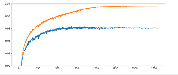
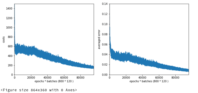
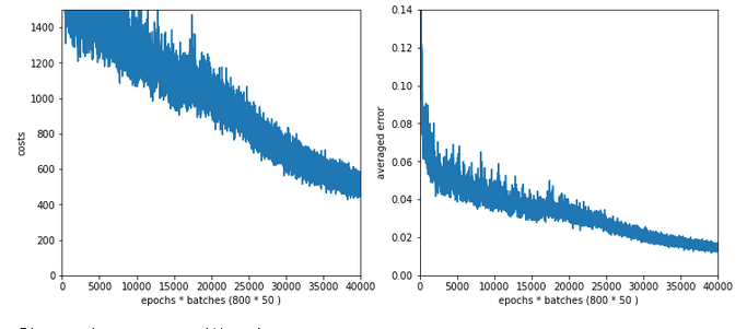
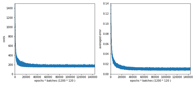
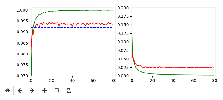
Below I show screenshots taken during training for the parameters defined above.


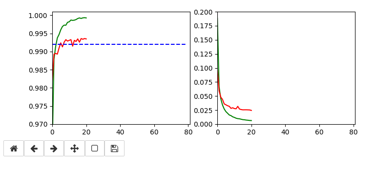
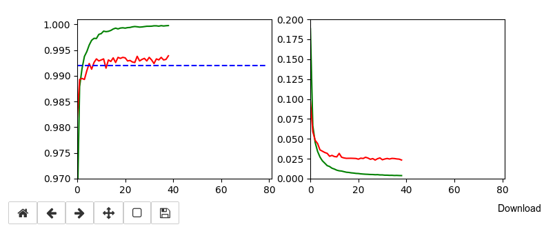
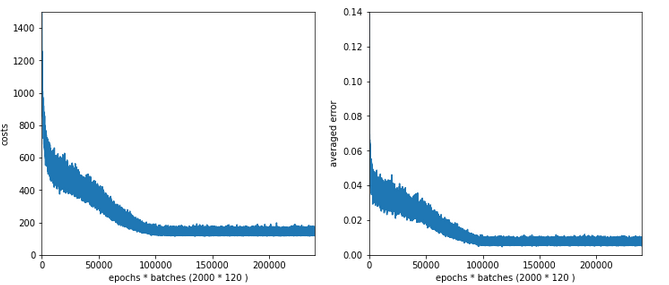
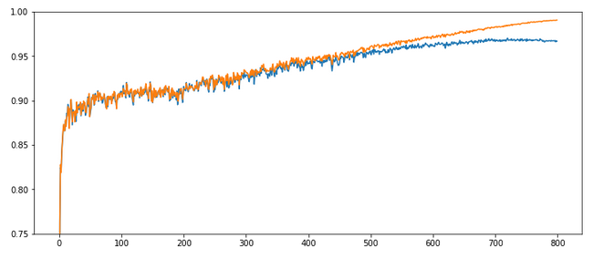
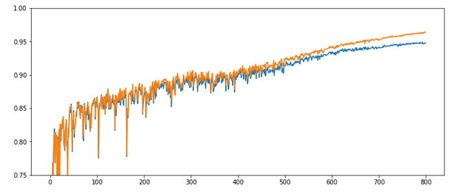
The left plot shows the achieved accuracy; red for the validation set (around 99.32%). The right plot shows the decline of the loss function relative to the original value. The green lines are for the training data, the red for the validation data.

Besides the effect of seeing the data change and the plots evolve during data, we can also take the result with us that we have improved the accuracy already from 99.0% to 99.32%. When you play around with the available hyperparameters a bit you may find that 99.25% is a reproducible accuracy. But in some cases you may reach 99.4% as best values.

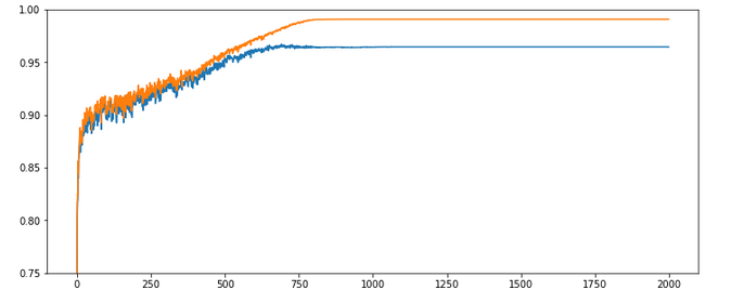
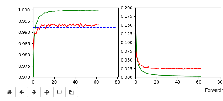
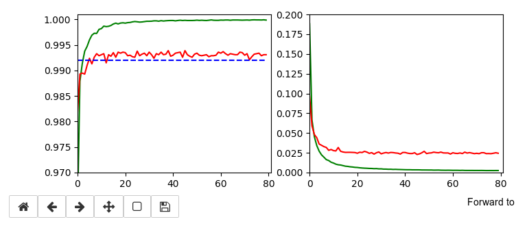
The following plots have best values around 99.4% with an average above 99.35%.

Epoch 13/80
935/938 [============================>.] - ETA: 0s - loss: 0.0096 - accuracy: 0.9986
present lr:  7.57920279e-05
present iteration: 12194
938/938 [==============================] - 6s 6ms/step - loss: 0.0096 - accuracy: 0.9986 - val_loss: 0.0238 - val_accuracy: 0.9944
Epoch 19/80
937/938 [============================>.] - ETA: 0s - loss: 0.0064 - accuracy: 0.9993
present lr:  5.3129319e-05
present iteration: 17822
938/938 [==============================] - 6s 6ms/step - loss: 0.0064 - accuracy: 0.9993 - val_loss: 0.0245 - val_accuracy: 0.9942
Epoch 22/80
930/938 [============================>.] - ETA: 0s - loss: 0.0056 - accuracy: 0.9994
present lr:  4.6219262e-05
present iteration: 20636
938/938 [==============================] - 6s 6ms/step - loss: 0.0056 - accuracy: 0.9994 - val_loss: 0.0238 - val_accuracy: 0.9942
Epoch 30/80
937/938 [============================>.] - ETA: 0s - loss: 0.0043 - accuracy: 0.9996
present lr:  3.43170905e-05
present iteration: 28140
938/938 [==============================] - 6s 6ms/step - loss: 0.0043 - accuracy: 0.9997 - val_loss: 0.0239 - val_accuracy: 0.9941
Epoch 55/80
937/938 [============================>.] - ETA: 0s - loss: 0.0028 - accuracy: 0.9998
present lr:  1.
90150222e-05
present iteration: 51590
938/938 [==============================] - 6s 6ms/step - loss: 0.0028 - accuracy: 0.9998 - val_loss: 0.0240 - val_accuracy: 0.9940
Epoch 69/80
936/938 [============================>.] - ETA: 0s - loss: 0.0025 - accuracy: 0.9999
present lr:  1.52156063e-05
present iteration: 64722
938/938 [==============================] - 6s 6ms/step - loss: 0.0025 - accuracy: 0.9999 - val_loss: 0.0245 - val_accuracy: 0.9940
Epoch 70/80
933/938 [============================>.] - ETA: 0s - loss: 0.0024 - accuracy: 0.9999
present lr:  1.50015e-05
present iteration: 65660
938/938 [==============================] - 6s 6ms/step - loss: 0.0024 - accuracy: 0.9999 - val_loss: 0.0245 - val_accuracy: 0.9940
Epoch 76/80
937/938 [============================>.] - ETA: 0s - loss: 0.0024 - accuracy: 0.9999
present lr:  1.38335554e-05
present iteration: 71288
938/938 [==============================] - 6s 6ms/step - loss: 0.0024 - accuracy: 0.9999 - val_loss: 0.0237 - val_accuracy: 0.9943


Parameters of the last run were

build = True
if cnn == None:
    build = True
    x_optimizer = None 

batch_size=64
epochs=80
reset = True 

my_loss    ='categorical_crossentropy'
my_metrics =['accuracy']
my_regularizer = None
my_regularizer = 'l2'
my_reg_param_l2 = 0.0008
my_reg_param_l1 = 0.01

my_optimizer      = 'rmsprop'       # Present alternatives:  rmsprop, nadam, adamax 
my_momentum       = 0.5            # momentum value 
my_lr_sched       = 'powerSched'    # Present alternatrives: None, powerSched, exponential 
#my_lr_sched       = None           # Present alternatrives: None, powerSched, exponential 
my_lr_init        = 0.001           # initial leaning rate  
my_lr_decay_steps = 1               # decay steps = 1 
my_lr_decay_rate  = 0.001           # decay rate 

li_conv_1   = [64, (3,3), 0] 
li_conv_2   = [64, (3,3), 0] 
li_conv_3   = [128, (3,3), 0] 
li_Conv     = [li_conv_1, li_conv_2, li_conv_3]
li_pool_1   = [(2,2)]
li_pool_2   = [(2,2)]
li_Pool     = [li_pool_1, li_pool_2]
li_dense_1  = [120, 0]
#li_dense_2  = [30, 0]
li_dense_3  = [10, 0]
li_MLP      = [li_dense_1, li_dense_2, li_dense_3]
li_MLP      = [li_dense_1, li_dense_3]
input_shape = (28,28,1)

 
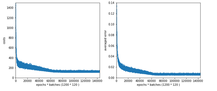
It is interesting that RMSProp only requires small values of the L2-regularizer for a sufficient stabilization – such that the loss curve for the validation data does not rise again substantially. Instead we observe an oscillation around a minimum after the learning rate as decreased sufficiently.

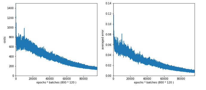
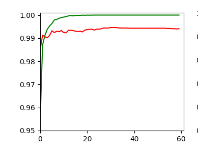
Addendum, 15.06.2020

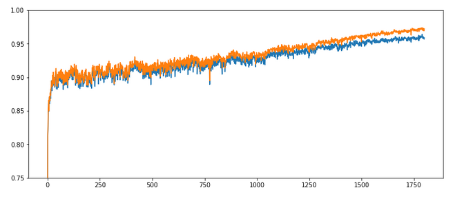
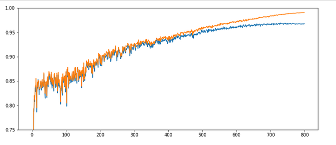
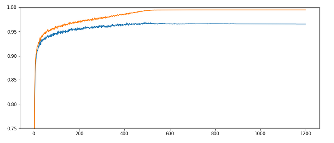
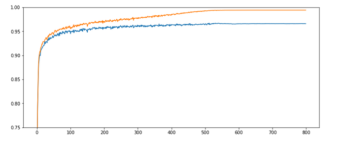
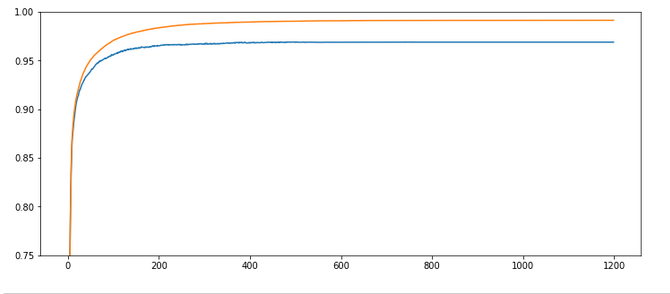
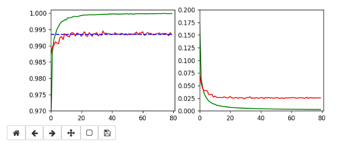
An attentive reader has found out that I have cheated a bit: I have used 64 maps at the first convolutional layer instead of 32 according to the setup in the previous article. Yes, sorry. To compensate for this I include the plot of a run with 32 maps at the first convolution. The blue line marks an accuracy of 99.35%. You see that we can get above it with 32 maps, too.

The parameters were:

build = True
if cnn == None:
    build = True
    x_optimizer = None 
batch_size=64
epochs=80
reset = False # reset the initial weight values to those saved?  

my_loss    ='categorical_crossentropy'
my_metrics =['accuracy']

my_regularizer = None
my_regularizer = 'l2'
my_reg_param_l2 = 0.001
#my_reg_param_l2 = 0.01
my_reg_param_l1 = 0.01

my_
optimizer      = 'rmsprop'       # Present alternatives:  rmsprop, nadam, adamax 
my_momentum       = 0.9           # momentum value 
my_lr_sched       = 'powerSched'    # Present alternatrives: None, powerSched, exponential 
#my_lr_sched       = None           # Present alternatrives: None, powerSched, exponential 
my_lr_init        = 0.001           # initial leaning rate  
my_lr_decay_steps = 1               # decay steps = 1 
my_lr_decay_rate  = 0.001           # decay rate 

li_conv_1    = [32, (3,3), 0] 
li_conv_2    = [64, (3,3), 0] 
li_conv_3    = [128, (3,3), 0] 
li_Conv      = [li_conv_1, li_conv_2, li_conv_3]
li_Conv_Name = ["Conv2D_1", "Conv2D_2", "Conv2D_3"]
li_pool_1    = [(2,2)]
li_pool_2    = [(2,2)]
li_Pool      = [li_pool_1, li_pool_2]
li_Pool_Name = ["Max_Pool_1", "Max_Pool_2", "Max_Pool_3"]
li_dense_1   = [120, 0]
#li_dense_2  = [30, 0]
li_dense_3   = [10, 0]
li_MLP       = [li_dense_1, li_dense_2, li_dense_3]
li_MLP       = [li_dense_1, li_dense_3]
input_shape  = (28,28,1)


Epoch 15/80
926/938 [============================>.] - ETA: 0s - loss: 0.0095 - accuracy: 0.9988
present lr:  6.6357e-05
present iteration: 14070
938/938 [==============================] - 4s 5ms/step - loss: 0.0095 - accuracy: 0.9988 - val_loss: 0.0268 - val_accuracy: 0.9940
Epoch 23/80
935/938 [============================>.] - ETA: 0s - loss: 0.0067 - accuracy: 0.9995
present lr:  4.42987512e-05
present iteration: 21574
938/938 [==============================] - 4s 5ms/step - loss: 0.0066 - accuracy: 0.9995 - val_loss: 0.0254 - val_accuracy: 0.9943
Epoch 35/80
936/938 [============================>.] - ETA: 0s - loss: 0.0049 - accuracy: 0.9996
present lr:  2.95595619e-05
present iteration: 32830
938/938 [==============================] - 4s 5ms/step - loss: 0.0049 - accuracy: 0.9996 - val_loss: 0.0251 - val_accuracy: 0.9945

Another stupid thing, which I should have mentioned:
I have not yet found a simple way of how to explicitly reset the number of iterations, only,

  • without a recompilation
  • or reloading a fully saved model at iteration 0 instead of reloading only the weights
  • or writing my own scheduler class based on epochs or batches.

With the present code you would have to (re-) build the model to avoid starting with a large number of “iterations” – and thus a small learning-rate in a second training run. My “reset”-parameter alone does not help.

By the way: Shape of the weight matrices

Some of my readers may be tempted to have a look at the weight tensors. This is possible via the optimizer and a callback. Then they may wonder about the dimensions, which are logically a bit different from the weight matrices I have used in my code for MLPs in another article series.

In the last article of this CNN series I have mentioned that Keras takes care of configuring the weight matrices itself as soon as it got all information about the layers and layers’ nodes (or units). Now, this still leaves some open degrees of handling the enumeration of layers and matrices; it is plausible that the logic of the layer and weight association must follow a convention. E.g., you can associate a weight matrix with the receiving layer in forward propagation direction. This is what Keras and TF2 do and it is different from what I did in my MLP code. Even if you have fixed this point, then you still can discuss the row/column-layout (shape) of the weight matrix:

Keras and TF2 require the “input_shape” i.e. the shape of the tensor which is fed into the present layer. Regarding the weight matrix it is the number of nodes (units) of the previous layer (in FW direction) which is interesting – normally this is given by the 2nd dimension number of the tensors shape. This has to be combined with the number of units in the present
layer. The systematics is that TF2 and Keras define the weight matrix between two layers according to the following convention for two adjacent layers L_N and L_(N+1) in FW direction:

L_N with A nodes (6 units) and L_(N+1) with B nodes (4 units) give a shape of the weight matrix as (A,B). [(6,4)]

See the references at the bottom of the article.

Note that this is NOT what we would expect from our handling of the MLP. However, the amount of information kept in the matrix is, of course, the same. It is just a matter of convention and array transposition for the required math operations during forward and error backward propagation. If you (for reasons of handling gradients) concentrate on BW propagation then the TF2/Keras convention is quite reasonable.

Conclusion

The Keras framework gives you access to a variety of hyperparameters you can use to control the use of a regularizer, the optimizer, the decline of the learning rate with batches/epochs, the momentum. The handling is a bit unconventional, but one gets pretty fast used to it.

We once again learned that it pays to invest a bit in a variation of such parameters, when you want to fight for the last tenth of percents beyond 99.0% accuracy. In the case of MNIST we can drive accuracy to 99.35%.

With the next article of this series

A simple CNN for the MNIST dataset – IV – Visualizing the activation output of convolutional layers and maps

we turn more to the question of visualizing some data at the convolutional layers to better understand their working.

Links

Layers and the shape of the weight matrices
https://keras.io/guides/sequential_model/
https://stackoverflow.com/questions/ 44791014/ understanding-keras-weight-matrix-of-each-layers
https://keras.io/guides/ making new layers and models via subclassing/

Learning rate and adaptive optimizers
https://towardsdatascience.com/learning-rate-schedules-and-adaptive-learning-rate-methods-for-deep-learning-2c8f433990d1
https://machinelearningmastery.com/ understand-the-dynamics-of-learning-rate-on-deep-learning-neural-networks/
https://faroit.com/keras-docs/2.0.8/optimizers/
https://keras.io/api/optimizers/
https://keras.io/api/optimizers/ learning_rate_schedules/
https://www.jeremyjordan.me/nn-learning-rate/

Keras Callbacks
https://keras.io/api/callbacks/
https://keras.io/guides/ writing_your_own_callbacks/
https://keras.io/api/callbacks/ learning_rate_scheduler/

Interactive plotting
https://stackoverflow.com/questions/ 39428347/ interactive-matplotlib-plots-in-jupyter-notebook
https://matplotlib.org/3.2.1/api/ _as_gen/ matplotlib.pyplot.ion.html
https://matplotlib.org/3.1.3/tutorials/ introductory/ usage.html

Further articles in this series

A simple CNN for the MNIST dataset – XI – Python code for filter visualization and OIP detection
A simple CNN for the MNIST dataset – X – filling some gaps in filter visualization
A simple CNN for the MNIST dataset – IX – filter visualization at a convolutional layer
A simple CNN for the MNIST dataset – VIII – filters and features – Python code to visualize patterns which activate a map strongly
A simple CNN for the MNIST dataset – VII – outline of steps to visualize image patterns which trigger filter maps
A simple CNN for the MNIST dataset – VI – classification by activation patterns and the role of the CNN’s MLP part
A simple CNN for the MNIST dataset – V – about the difference of activation patterns and features


A simple Python program for an ANN to cover the MNIST dataset – XII – accuracy evolution, learning rate, normalization

We continue our article series on building a Python program for a MLP and training it to recognize handwritten digits on images of the MNIST dataset.

A simple Python program for an ANN to cover the MNIST dataset – XI – confusion matrix
A simple Python program for an ANN to cover the MNIST dataset – X – mini-batch-shuffling and some more tests
A simple Python program for an ANN to cover the MNIST dataset – IX – First Tests
A simple Python program for an ANN to cover the MNIST dataset – VIII – coding Error Backward Propagation
A simple Python program for an ANN to cover the MNIST dataset – VII – EBP related topics and obstacles
A simple Python program for an ANN to cover the MNIST dataset – VI – the math behind the „error back-propagation“
A simple Python program for an ANN to cover the MNIST dataset – V – coding the loss function
A simple Python program for an ANN to cover the MNIST dataset – IV – the concept of a cost or loss function
A simple Python program for an ANN to cover the MNIST dataset – III – forward propagation
A simple Python program for an ANN to cover the MNIST dataset – II – initial random weight values
A simple Python program for an ANN to cover the MNIST dataset – I – a starting point

In the last article we used our prediction data to build a so called “confusion matrix” after training. With its help we got an overview about the “false negative” and “false positive” cases, i.e. cases of digit-images for which the algorithm made wrong predictions. We also displayed related critical MNIST images for the digit “4”.

In this article we first want to extend the ability of our class “ANN” such that we can measure the level of accuracy (more precisely: the recall) on the full test and the training data sets during training. We shall see that the resulting curves will trigger some new insights. We shall e.g. get an answer to the question at which epoch the accuracy on the test data set does no longer change, but the accuracy on the training set still improves. Meaning: We can find out after which epoch we spend CPU time on overfitting.

In addition we want to investigate the efficiency of our present approach a bit. So far we have used a relatively small learning rate of 0.0001 with a decrease rate of 0.000001. This gave us relatively smooth curves during convergence. However, it took us a lot of epochs and thus computational time to arrive at a cost
minimum. The question is:

Is a small learning rate really required? What happens if we use bigger initial learning rates? Can we reduce the number of epochs until learning converges?

Regarding the last point we should not forget that a bigger learning rate may help to move out of local minima on our way to the vicinity of a global minimum. Some of our experiments will indeed indicate that one may get stuck somewhere before moving deep into a minimum valley. However, our forthcoming experiments will also show that we have to take care about the weight initialization. And this in turn will lead us to a major deficit of our present code. Resolving it will help us with bigger learning rates, too.

Class interface changes

We introduce some new parameters, whose usage will become clear later on. They are briefly documented within the code. In addition we do no longer call the method _fit() automatically when we create a Python object instance of the class. This means the you have to call “_fit()” on your own in your Jupyter cells in the future.

To be able to use some additional features later on we first need some more import statements.

New import statements of the class MyANN

import numpy as np
import math 
import sys
import time
import tensorflow
# from sklearn.datasets import fetch_mldata
from sklearn.datasets import fetch_openml
from sklearn.metrics import confusion_matrix
from sklearn.preprocessing import StandardScaler

from sklearn.cluster import KMeans
from sklearn.cluster import MiniBatchKMeans

from keras.datasets import mnist as kmnist
from scipy.special import expit  
from matplotlib import pyplot as plt
from symbol import except_clause
from IPython.core.tests.simpleerr import sysexit
from math import floor


Extended My_ANN interface
We extend our interface substantially – although we shall not use every new parameter, yet. Most of the parameters are documented shortly; but to really understand what they control you have to look into some other changed parts of the class’s code, which we present later on. You can, however, safely ignore parameters on “clustering” and “PCA” in this article. We shall yet neither use the option to import MNIST X- and y-data (X_import, y_import) instead of loading them internally.

    
    def __init__(self, 
                 my_data_set = "mnist",
                 
                 X_import = None, # imported X dataset 
                 y_import = None, # imported y dataset 
                 
                 num_test_records = 10000, # number of test data 
                 
                 # parameter for normalization of input data 
                 b_normalize_X = False, # True: apply StandardScaler on X input data
                 
                 # parameters for clustering of input data 
                 b_perform_clustering = False,  # shall we cluster the X_data before learning? 
                 my_clustering_method = "MiniBatchKMeans", # Choice between 2 methods: MiniBatchKMeans, KMeans  
                 cl_n_clusters = 200,      # number of clusters (often "k" in literature)
                 cl_max_iter = 600,        # number of iterations for centroid movement
                 cl_n_init = 100,          # number of different initial centroid positions tried 
                 cl_n_jobs = 4,            # number of CPU cores (jobs to start for investigating n_init variations
                 cl_batch_size = 500,      # batch size, only used for MiniBatchKMeans
                 
                 #parameters for PCA of input data 
                 b_
perform_pca = False,
                 num_pca_categories = 155, 
                 
                 # parameters for MLP structure
                 n_hidden_layers = 1, 
                 ay_nodes_layers = [0, 100, 0], # array which should have as much elements as n_hidden + 2
                 n_nodes_layer_out = 10,  # expected number of nodes in output layer 
                                                  
                 my_activation_function = "sigmoid", 
                 my_out_function        = "sigmoid",   
                 my_loss_function       = "LogLoss",   
                 
                 n_size_mini_batch = 50,  # number of data elements in a mini-batch 
                 
                 n_epochs      = 1,
                 n_max_batches = -1,  # number of mini-batches to use during epochs - > 0 only for testing 
                                      # a negative value uses all mini-batches 
                 
                 lambda2_reg = 0.1,     # factor for quadratic regularization term 
                 lambda1_reg = 0.0,     # factor for linear regularization term 
                 
                 vect_mode = 'cols', 
                 
                 init_weight_meth_L0 = "sqrt_nodes",  # method to init weights => "sqrt_nodes", "const"
                 init_weight_meth_Ln = "sqrt_nodes",  # sqrt_nodes", "const"
                 init_weight_intervals = [(-0.5, 0.5), (-0.5, 0.5), (-0.5, 0.5)],   # size must fit number of hidden layers
                 init_weight_fact = 2.0,                # extends the interval 
                 
                 
                 learn_rate = 0.001,          # the learning rate (often called epsilon in textbooks) 
                 decrease_const = 0.00001,    # a factor for decreasing the learning rate with epochs
                 learn_rate_limit = 2.0e-05,  # a lower limit for the learn rate 
                 adapt_with_acc = False,      # adapt learning rate with additional factor depending on rate of acc change
                 reduction_fact = 0.001,      # small reduction factor - should be around 0.001 because of an exponential reduction
                 
                 mom_rate   = 0.0005,         # a factor for momentum learning
                 
                 b_shuffle_batches = True,    # True: we mix the data for mini-batches in the X-train set at the start of each epoch
                 
                 b_predictions_train = False, # True: At the end of periodic epochs the code performs predictions on the train data set
                 b_predictions_test  = False, # True: At the end of periodic epochs the code performs predictions on the test data set
                 prediction_test_period  = 1, # Period of epochs for which we perform predictions
                 prediction_train_period = 1, # Period of epochs for which we perform predictions
                 
                 print_period = 20,         # number of epochs for which to print the costs and the averaged error
                 
                 figs_x1=12.0, figs_x2=8.0, 
                 legend_loc='upper right',
                 
                 b_print_test_data = True
                 
                 ):
        '''
        Initialization of MyANN
        Input: 
            data_set: type of dataset; so far only the "mnist", "mnist_784" datsets are known 
                      We use this information to prepare the input data and learn about the feature dimension. 
                      This info is used in preparing the size of the input layer.     
            
            X_import: external X dataset to import  
            y_import: external y dataset to import - must fit in dimension to X_import 
            
            num_test_records: number of test data
            
            b_normalize_X: True => Invoke the StandardScaler of 
Scikit-Learn 
                                   to center and normalize the input data X
            
            Preprocessing of input data treatment before learning 
            ------------------------------------
            Clustering
            -----------
            b_perform_clustering   # True => Cluster the X_data before learning? 
            my_clustering_method   # string: 2 methods: MiniBatchKMeans, KMeans 
            cl_n_clusters = 200       # number of clusters (often "k" in literature)
            cl_max_iter = 600      # number of iterations for centroid movement
            cl_n_init = 100        # number of different initial centroid positions tried 
            cl_n_jobs = 4,         # number of CPU cores => jobs - only used for "KMeans"
            cl_batch_size = 500    # batch size used for "MiniBatchKMeans"
            
            PCA
            -----
            b_perform_pca: True => perform a pca analysis 
            num_pca_categories: 155 - choose a reasonable number 
            
            n_hidden_layers = number of hidden layers => between input layer 0 and output layer n 
            
            ay_nodes_layers = [0, 100, 0 ] : We set the number of nodes in input layer_0 and the output_layer to zero 
                              Will be set to real number afterwards by infos from the input dataset. 
                              All other numbers are used for the node numbers of the hidden layers.
            n_nodes_out_layer = expected number of nodes in the output layer (is checked); 
                                this number corresponds to the number of categories NC = number of labels to be distinguished
            
            my_activation_function : name of the activation function to use 
            my_out_function : name of the "activation" function of the last layer which produces the output values 
            my_loss_function : name of the "cost" or "loss" function used for optimization 
            
            n_size_mini_batch : Number of elements/samples in a mini-batch of training data 
                                The number of mini-batches will be calculated from this
            
            n_epochs : number of epochs to calculate during training
            n_max_batches : > 0: maximum of mini-batches to use during training 
                            < 0: use all mini-batches  
            
            lambda_reg2:    The factor for the quadartic regularization term 
            lambda_reg1:    The factor for the linear regularization term 
            
            vect_mode: Are 1-dim data arrays (vctors) ordered by columns or rows ?
            
            init_weight_meth_L0: Method to calculate the initial weights at layer L0: "sqrt_nodes" => sqrt(number of nodes) /  "const" => interval borders 
            init_weight_meth_Ln: Method to calculate the initial weights at hidden layers 
            init_weight_intervals: list of tuples with interval limits [(-0.5, 0.5), (-0.5, 0.5), (-0.5, 0.5)],   
                                   size must fit number of hidden layers
            init_weight_fact:  interval limits get scald by this factor, e.g. 2* (0,5, 0.5)

            learn rate :     Learning rate - definies by how much we correct weights in the indicated direction of the gradient on the cost hyperplane.
            decrease_const:  Controls a systematic decrease of the learning rate with epoch number 
            learn_rate_limit = 2.0e-05,  # a lowee limit for the learning rate 
            
            adapt_with_acc:  True => adapt learning rate with additional factor depending on rate of acc change
            reduction_fact:  around 0.001  => almost exponential reduction during the first 500 epochs   
            
            mom_const:       Momentum rate. Controls a mixture of the last with the present weight 
corrections (momentum learning)
            
            b_shuffle_batches: True => vary composition of mini-batches with each epoch
            
            # The next two parameters enable the measurement of accuracy and total cost function 
            # by making predictions on the train and test datasets 
            b_predictions_train: True => perform a prediction run on the full training data set => get accuracy 
            b_predictions_test:  True => perform a prediction run on the full test data set => get accuracy 
            prediction_test_period: period of epochs for which to perform predictions
            prediction_train_period: period of epochs for which to perform predictions
            
            print_period:    number of periods between printing out some intermediate data 
                             on costs and the averaged error of the last mini-batch   
                       
            
            figs_x1=12.0, figs_x2=8.0 : Standard sizing of plots , 
            legend_loc='upper right': Position of legends in the plots
            
            b_print_test_data: Boolean variable to control the print out of some tests data 
             
         '''
        
        # Array (Python list) of known input data sets 
        self._input_data_sets = ["mnist", "mnist_784", "mnist_keras", "imported"]  
        self._my_data_set = my_data_set
        
        # X_import, y_import, X, y, X_train, y_train, X_test, y_test  
            # will be set by method handle_input_data() 
            # X: Input array (2D) - at present status of MNIST image data, only.    
            # y: result (=classification data) [digits represent categories in the case of Mnist]
        self._X_import = X_import 
        self._y_import = y_import 
        
        # number of test data 
        self._num_test_records = num_test_records
        
        self._X       = None 
        self._y       = None 
        self._X_train = None 
        self._y_train = None 
        self._X_test  = None   
        self._y_test  = None
        
        # perform a normalization of the input data
        self._b_normalize_X = b_normalize_X
        
        # relevant dimensions 
        # from input data information;  will be set in handle_input_data()
        self._dim_X        = 0  # total num of records in the X,y input sets
        self._dim_sets     = 0  # num of records in the TRAINING sets X_train, y_train
        self._dim_features = 0  
        self._n_labels     = 0   # number of unique labels - will be extracted from y-data 
        
        # Img sizes 
        self._dim_img      = 0 # should be sqrt(dim_features) - we assume square like images  
        self._img_h        = 0 
        self._img_w        = 0 
        
        # Preprocessing of input data 
        # ---------------------------
        self._b_perform_clustering = b_perform_clustering
        self._my_clustering_method = my_clustering_method # for the related dictionary see below 
        self._kmeans        = None   # pointer to object used for clustering  
        self._cl_n_clusters = cl_n_clusters       # number of clusters (often "k" in literature)
        self._cl_max_iter   = cl_max_iter      # number of iterations for centroid movement
        self._cl_n_init     = cl_n_init        # number of different initial centroid positions tried 
        self._cl_batch_size = cl_batch_size    # batch size used for MiniBatchKMeans
        self._cl_n_jobs     = cl_n_jobs        # number of parallel jobs (on CPU-cores) - only used for KMeans
        
        # Layers
        # ------
        # number of hidden layers 
        self._n_hidden_layers = n_hidden_layers
        # Number of total layers 
        self._n_total_layers = 2 + self._n_hidden_layers  
        # Nodes for hidden layers 
        
self._ay_nodes_layers = np.array(ay_nodes_layers)
        # Number of nodes in output layer - will be checked against information from target arrays
        self._n_nodes_layer_out = n_nodes_layer_out
        
        # Weights 
        # --------
        # empty List for all weight-matrices for all layer-connections
        # Numbering : 
        # w[0] contains the weight matrix which connects layer 0 (input layer ) to hidden layer 1 
        # w[1] contains the weight matrix which connects layer 1 (input layer ) to (hidden?) layer 2 
        self._li_w = []
        
        # Arrays for encoded output labels - will be set in _encode_all_mnist_labels()
        # -------------------------------
        self._ay_onehot = None
        self._ay_oneval = None
        
        # Known Randomizer methods ( 0: np.random.randint, 1: np.random.uniform )  
        # ------------------
        self.__ay_known_randomizers = [0, 1]

        # Types of activation functions and output functions 
        # ------------------
        self.__ay_activation_functions = ["sigmoid"] # later also relu 
        self.__ay_output_functions     = ["sigmoid"] # later also softmax 
        
        # Types of cost functions 
        # ------------------
        self.__ay_loss_functions = ["LogLoss", "MSE" ] # later also other types of cost/loss functions  


        # dictionaries for indirect function calls 
        self.__d_activation_funcs = {
            'sigmoid': self._sigmoid, 
            'relu':    self._relu
            }
        self.__d_output_funcs = { 
            'sigmoid': self._sigmoid, 
            'softmax': self._softmax
            }  
        self.__d_loss_funcs = { 
            'LogLoss': self._loss_LogLoss, 
            'MSE': self._loss_MSE
            }  
        # Derivative functions 
        self.__d_D_activation_funcs = {
            'sigmoid': self._D_sigmoid, 
            'relu':    self._D_relu
            }
        self.__d_D_output_funcs = { 
            'sigmoid': self._D_sigmoid, 
            'softmax': self._D_softmax
            }  
        self.__d_D_loss_funcs = { 
            'LogLoss': self._D_loss_LogLoss, 
            'MSE': self._D_loss_MSE
            }  
        self.__d_clustering_functions = {
            'MiniBatchKMeans': self._Mini_Batch_KMeans, 
            'KMeans': self._KMeans
            } 
        
        # The following variables will later be set by _check_and set_activation_and_out_functions()            
        self._my_act_func  = my_activation_function
        self._my_out_func  = my_out_function
        self._my_loss_func = my_loss_function
        self._act_func      = None    
        self._out_func      = None    
        self._loss_func     = None    
        self._cluster_func  = None    
        
        # number of data samples in a mini-batch 
        self._n_size_mini_batch = n_size_mini_batch
        self._n_mini_batches = None  # will be determined by _get_number_of_mini_batches()

        # maximum number of epochs - we set this number to an assumed maximum 
        # - as we shall build a backup and reload functionality for training, this should not be a major problem 
        self._n_epochs = n_epochs
        
        # maximum number of batches to handle ( if < 0 => all!) 
        self._n_max_batches = n_max_batches
        # actual number of batches 
        self._n_batches = None

        # regularization parameters
        self._lambda2_reg = lambda2_reg
        self._lambda1_reg = lambda1_reg
        
        # parameters to control the initialization of the weights (see _create_WM_Input(), create_WM_Hidden())
        self._init_weight_meth_L0 = init_weight_meth_L0
        self._init_weight_meth_Ln = init_weight_meth_Ln
        self._init_weight_
intervals = init_weight_intervals # list of lists with interval borders
        self._init_weight_fact = init_weight_fact           # extends weight intervals 
        
        
        # parameters for adaption of the learning rate
        self._learn_rate = learn_rate
        self._decrease_const = decrease_const
        self._learn_rate_limit = learn_rate_limit
        self._adapt_with_acc  = adapt_with_acc
        self._reduction_fact  = reduction_fact
        #
        # parameters for momentum learning 
        self._mom_rate   = mom_rate
        self._li_mom = [None] *  self._n_total_layers
        
        # shuffle data in X_train? 
        self._b_shuffle_batches = b_shuffle_batches
        
        # perform predictions on train and test data set and related analysis 
        self._b_predictions_train = b_predictions_train
        self._b_predictions_test  = b_predictions_test
        self._prediction_test_period  = prediction_test_period
        self._prediction_train_period = prediction_train_period
        
        # epoch period for printing 
        self._print_period = print_period
        
        # book-keeping for epochs and mini-batches 
        # -------------------------------
        # range for epochs - will be set by _prepare-epochs_and_batches() 
        self._rg_idx_epochs = None
        # range for mini-batches 
        self._rg_idx_batches = None
        # dimension of the numpy arrays for book-keeping - will be set in _prepare_epochs_and_batches() 
        self._shape_epochs_batches = None    # (n_epochs, n_batches, 1) 

        # training evolution:
        # +++++++++++++++++++ 
        # List for error values at outermost layer for minibatches and epochs during training
        # we use a numpy array here because we can redimension it
        self._ay_theta = None
        # List for cost values of mini-batches during training - The list will later be split into sections for epochs 
        self._ay_costs = None
        #
        # List for test accuracy values and error values at epoch periods 
        self._ay_period_test_epoch = None # x-axis for plots of the following 2 quantities 
        self._ay_acc_test_epoch = None  
        self._ay_err_test_epoch = None  
        # List for train accuracy values and error values at epoch periods  
        self._ay_period_train_epoch = None # x-axis for plots of the following 2 quantities 
        self._ay_acc_train_epoch = None  
        self._ay_err_train_epoch = None  
        
        # Data elements for back propagation
        # ----------------------------------
        
        # 2-dim array of partial derivatives of the elements of an additive cost function 
        # The derivative is taken with respect to the output results a_j = ay_ANN_out[j]
        # The array dimensions account for nodes and sampls of a mini_batch. The array will be set in function 
        # self._initiate_bw_propagation()
        self._ay_delta_out_batch = None
        

        # parameter to allow printing of some test data 
        self._b_print_test_data = b_print_test_data

        # Plot handling 
        # --------------
        # Alternatives to resize plots 
        # 1: just resize figure  2: resize plus create subplots() [figure + axes] 
        self._plot_resize_alternative = 1 
        # Plot-sizing
        self._figs_x1 = figs_x1
        self._figs_x2 = figs_x2
        self._fig = None
        self._ax  = None 
        # alternative 2 does resizing and (!) subplots() 
        self.initiate_and_resize_plot(self._plot_resize_alternative)        
        
        
        # ***********
        # operations 
        # ***********
        
        # check and handle input data 
        self._handle_input_data()
        # set the ANN structure 
        self._set_ANN_structure()
        
     
   # Prepare epoch and batch-handling - sets ranges, limits num of mini-batches and initializes book-keeping arrays
        self._rg_idx_epochs, self._rg_idx_batches = self._prepare_epochs_and_batches()


Code modifications to create precise accuracy information on the full test and training sets during training

You certainly noticed the following set of control parameters in the class’s new interface:

  • b_predictions_train = False, # True: At the end of periodic epochs the code performs predictions on the train data set
  • b_predictions_test = False, # True: At the end of periodic epochs the code performs predictions on the test data set
  • prediction_test_period = 1, # Period of epochs for which we perform predictions
  • prediction_train_period = 1, # Period of epochs for which we perform predictions

These parameters control whether we perform predictions during training for the full test dataset and/or the full training dataset – and if so, at which epoch period. Actually, during all of the following experiments we shall evaluate the accuracy data after each single period.

We need an array to gather accuracy information. We therefore modify the method “_prepare_epochs_and_batches()”, where we fill some additional Numpy arrays with initialization values. Thus we avoid a costly “append()” later on; we just overwrite the array entries successively. This overwriting happens in our method _fit(); see below.

Changes to function “_prepare_epochs_and_batches()”:

    ''' -- Main Method to prepare epochs, batches and book-keeping arrays -- '''
    def _prepare_epochs_and_batches(self, b_print = True):
        # range of epochs
        ay_idx_epochs  = range(0, self._n_epochs)
        
        # set number of mini-batches and array with indices of input data sets belonging to a batch 
        self._set_mini_batches()
        
        # limit the number of mini-batches
        self._n_batches = min(self._n_max_batches, self._n_mini_batches)
        ay_idx_batches = range(0, self._n_batches)
        if (b_print):
            if  self._n_batches < self._n_mini_batches :
                print("\nWARNING: The number of batches has been limited from " + 
                      str(self._n_mini_batches) + " to " + str(self._n_max_batches) )
        
        # Set the book-keeping arrays 
        self._shape_epochs_batches = (self._n_epochs, self._n_batches)
        self._ay_theta = -1 * np.ones(self._shape_epochs_batches) # float64 numbers as default
        self._ay_costs = -1 * np.ones(self._shape_epochs_batches) # float64 numbers as default
        
        shape_test_epochs  = ( floor(self._n_epochs / self._prediction_test_period), )
        shape_train_epochs = ( floor(self._n_epochs / self._prediction_train_period), )
        self._ay_period_test_epoch  = -1 * np.ones(shape_test_epochs) # float64 numbers as default
        self._ay_acc_test_epoch     = -1 * np.ones(shape_test_epochs) # float64 numbers as default
        self._ay_err_test_epoch     = -1 * np.ones(shape_test_epochs) # float64 numbers as default
        self._ay_period_train_epoch = -1 * np.ones(shape_train_epochs) # float64 numbers as default
        self._ay_acc_train_epoch    = -1 * np.ones(shape_train_epochs) # float64 numbers as default
        self._ay_err_train_epoch    = -1 * np.ones(shape_train_epochs) # float64 numbers as default
        
        return ay_idx_epochs, ay_idx_batches 
#


We then create two new methods to calculate accuracy values by predicting results on all records of both the training dataset and the test dataset. The attentive reader certainly recognizes the methods’ structure from a previous article where we used
similar code in a Jupyter cell:

New functions “_predict_all_test_data()” and “_predict_all_train_data()”:

    ''' Method to predict values for the full set of test data '''
    def _predict_all_test_data(self): 
        size_set = self._X_test.shape[0]
    
        li_Z_in_layer_test  = [None] * self._n_total_layers
        li_Z_in_layer_test[0] = self._X_test
        
        # Transpose input data matrix  
        ay_Z_in_0T       = li_Z_in_layer_test[0].T
        li_Z_in_layer_test[0] = ay_Z_in_0T
        li_A_out_layer_test  = [None] * self._n_total_layers
    
        # prediction by forward propagation of the whole test set 
        self._fw_propagation(li_Z_in = li_Z_in_layer_test, li_A_out = li_A_out_layer_test, b_print = False) 
        ay_predictions_test = np.argmax(li_A_out_layer_test[self._n_total_layers-1], axis=0)
        
        # accuracy 
        ay_errors_test = self._y_test - ay_predictions_test 
        acc_test = (np.sum(ay_errors_test == 0)) / size_set
        # print ("total acc for test data = ", acc)
        # return acc, ay_predictions_test
        return acc_test
#
    ''' Method to predict values for the full set of training data '''
    def _predict_all_train_data(self): 
        size_set = self._X_train.shape[0]
    
        li_Z_in_layer_train  = [None] * self._n_total_layers
        li_Z_in_layer_train[0] = self._X_train
        # Transpose 
        ay_Z_in_0T       = li_Z_in_layer_train[0].T
        li_Z_in_layer_train[0] = ay_Z_in_0T
        li_A_out_layer_train  = [None] * self._n_total_layers
    
        self._fw_propagation(li_Z_in = li_Z_in_layer_train, li_A_out = li_A_out_layer_train, b_print = False) 
        ay_predictions_train = np.argmax(li_A_out_layer_train[self._n_total_layers-1], axis=0)
        ay_errors_train = self._y_train - ay_predictions_train 
        acc_train = (np.sum(ay_errors_train == 0)) / size_set
        #print ("total acc for train data = ", acc)    
        
        return acc_train
#


Eventually, we modify our method “_fit()” with a series of statements on the level of the epoch loop. You may ignore most of the statements for learning rate adaption; we only use the “simple” adaption methods. The really important changes are those regarding predictions.

Modifications of function “_fit()”:

    ''' -- Method to perform training in epochs for defined mini-batches -- '''
    def _fit(self, b_print = False, b_measure_epoch_time = True, b_measure_batch_time = False):
        '''
        Parameters: 
            b_print:                 Do we print intermediate results of the training at all? 
            b_print_period:          For which period of epochs do we print? 
            b_measure_epoch_time:    Measure CPU-Time for an epoch
            b_measure_batch_time:    Measure CPU-Time for a batch
        '''
        rg_idx_epochs  = self._rg_idx_epochs 
        rg_idx_batches = self._rg_idx_batches
        if (b_print):    
            print("\nnumber of epochs = " + str(len(rg_idx_epochs)))
            print("max number of batches = " + str(len(rg_idx_batches)))
        
        # Some intial parameters 
        acc_old = 0.0000001
        acc_test = 0.001
        orig_rate = self._learn_rate
        adapt_fact = 1.0
        n_predict_test  = 0
        n_predict_train = 0
        
        # loop over epochs
        # ****************
        start_train = time.perf_counter()
        for idxe in rg_idx_epochs:
            if b_print and (idxe % self._print_period == 0):
                if b_measure_epoch_time:
          
          start_0_e = time.perf_counter()
                print("\n ---------")
                print("Starting epoch " + str(idxe+1))
            
            # simple adaption of the learning rate 
            # ~~~~~~~~~~~~~~~~~~~~~~~~~~~~~~~~~~~~
            orig_rate /= (1.0 + self._decrease_const * idxe)
            self._learn_rate /= (1.0 + self._decrease_const * idxe)
            if self._learn_rate < self._learn_rate_limit:
                self._learn_rate = self._learn_rate_limit
            
            # adapt wit acc. - not working well, yet 
            #~~~~~~~~~~~~~~~~~~~~~~~~~~~~~~~~~~~~~~~
            acc_change_rate = math.fabs((acc_test - acc_old) / acc_old)
            if b_print and (idxe % self._print_period == 0):
                print("acc_chg_rate = ", acc_change_rate)
            ratio = self._learn_rate / orig_rate 
            if ratio > 0.33 and acc_change_rate < 1/3 and self._adapt_with_acc:
                if acc_change_rate < 0.001:
                    acc_change_rate = 0.001
                #adapt_fact = 2.0 * acc_change_rate / (1.0 - acc_change_rate)
                adapt_fact = 1.0 - 0.001 * (1.0 - acc_change_rate / (1.0 - acc_change_rate))
                if b_print and (idxe % self._print_period == 0):
                    print("adapt_fact = ", adapt_fact)
                self._learn_rate *= adapt_fact
            acc_old = acc_test # for adaption of learning rate 
            
            # shuffle indices for a variation of the mini-batches with each epoch
            # ******************************************************************
            if self._b_shuffle_batches:
                shuffled_index = np.random.permutation(self._dim_sets)
                self._X_train, self._y_train, self._ay_onehot = self._X_train[shuffled_index], self._y_train[shuffled_index], self._ay_onehot[:, shuffled_index]
            #
            # loop over mini-batches
            # **********************
            for idxb in rg_idx_batches:
                if b_measure_batch_time: 
                    start_0_b = time.perf_counter()
                # deal with a mini-batch
                self._handle_mini_batch(num_batch = idxb, num_epoch=idxe, b_print_y_vals = False, b_print = False)
                if b_measure_batch_time: 
                    end_0_b = time.perf_counter()
                    print('Time_CPU for batch ' + str(idxb+1), end_0_b - start_0_b) 
            
            #
            # predictions
            # ***********
            # Control and perform predictions on the full test data set 
            if self._b_predictions_test and idxe % self._prediction_test_period == 0:
                self._ay_period_test_epoch[n_predict_test] = idxe
                acc_test = self._predict_all_test_data()
                self._ay_acc_test_epoch[n_predict_test] = acc_test
                n_predict_test += 1
            # Control and perform predictions on the full training training data set 
            if self._b_predictions_train and idxe % self._prediction_train_period == 0:
                self._ay_period_train_epoch[n_predict_train] = idxe
                acc_train = self._predict_all_train_data()
                self._ay_acc_train_epoch[n_predict_train] = acc_train
                n_predict_train += 1
            #
            # printing some evolution and epoch information
            if b_print and (idxe % self._print_period == 0):
                if b_measure_epoch_time:
                    end_0_e = time.perf_counter()
                    print('Time_CPU for epoch' + str(idxe+1), end_0_e - start_0_e) 
                print("learning rate = ", self._learn_rate)
                print("orig learn rate = ", orig_rate)
                print("\ntotal costs of last mini_batch = ", self._ay_costs[idxe, idxb])
                print("avg total error of 
last mini_batch = ", self._ay_theta[idxe, idxb])
                # print presently reached accuracy values on the test and training sets 
                print("presently reached train accuracy =<div style="width: 95%; overflow: auto; height: 400px;">
<pre style="width: 1000px;">
 ", acc_train)
                print("presently reached test accuracy = ", acc_test)
                
        # print out required secs for training
        # **************************************
        end_train = time.perf_counter()
        print('\n\n ------') 
        print('Total training Time_CPU: ', end_train - start_train) 
        print("\nStopping program regularily")

        return None
#

 
The method we apply in the above code to reduce the learning rate with every epoch is by the way called “power scheduling“. The book of Aurelien Geron [“Hands on Machine learning ….”, 2019, 2nd edition, O’Reilly], quoted already in previous articles, lists a bunch of other methods, e.g. “exponential scheduling”, where we multiply the learning rate with a constant factor < 1 at every epoch.

A further change of code happens in the functions _create_WM_input() and _ceate_WM_hidden” to initiate weight values.

Modifications of functions _create_WM_input() and _create_WM_hidden”:
Addendum 25.03.2020: Changed _create_WM_hidden() because of errors in the code

    '''-- Method to create the weight matrix between L0/L1 --'''
    def _create_WM_Input(self):
        '''
        Method to create the input layer 
        The dimension will be taken from the structure of the input data 
        We need to fill self._w[0] with a matrix for conections of all nodes in L0 with all nodes in L1
        We fill the matrix with random numbers between [-1, 1] 
        '''
        # the num_nodes of layer 0 should already include the bias node 
        num_nodes_layer_0 = self._ay_nodes_layers[0]
        num_nodes_with_bias_layer_0 = num_nodes_layer_0 + 1 
        num_nodes_layer_1 = self._ay_nodes_layers[1] 
        
        # Set interval borders for randomizer 
        if self._init_weight_meth_L0 == "sqrt_nodes":  # sqrtr(nodes) - rule of Prof. J. Frochte
            rand_high = self._init_weight_fact / math.sqrt(float(num_nodes_layer_0))
            rand_low = - rand_high 
        else: 
            rand_low  = self._init_weight_intervals[0][0]
            rand_high = self._init_weight_intervals[0][1]
        print("\nL0: weight range [" + str(rand_low) + ", " + str(rand_high) + "]" )
        
        # fill the weight matrix at layer L0 with random values 
        randomizer = 1 # method np.random.uniform   
        rand_size = num_nodes_layer_1 * (num_nodes_with_bias_layer_0) 
        w0 = self._create_vector_with_random_values(rand_low, rand_high, rand_size, randomizer)
        w0 = w0.reshape(num_nodes_layer_1, num_nodes_with_bias_layer_0)
        
        # put the weight matrix into array of matrices 
        self._li_w.append(w0)
        print("\nShape of weight matrix between layers 0 and 1 " + str(self._li_w[0].shape))
        
#
    '''-- Method to create the weight-matrices for hidden layers--''' 
    def _create_WM_Hidden(self):
        '''
        Method to create the weights of the hidden layers, i.e. between [L1, L2] and so on ... [L_n, L_out] 
        We fill the matrix with random numbers between [-1, 1] 
        '''
        
        # The "+1" is required due to range properties ! 
        rg_hidden_layers = range(1, self._n_hidden_layers + 1, 1)
        
        # Check parameter input fro weight intervals 
        if self._init_weight_meth_Ln == "const":
            if len(self._init_
weight_intervals) != (self._n_hidden_layers + 1):
                print("\nError: we shall initialize weights with values from intervals, but wrong number of intervals provided!") 
                sys.exit()
        
        for i in rg_hidden_layers: 
            print ("\nCreating weight matrix for layer " + str(i) + " to layer " + str(i+1) )
            
            num_nodes_layer = self._ay_nodes_layers[i] 
            num_nodes_with_bias_layer = num_nodes_layer + 1 

            # Set interval borders for randomizer 
            if self._init_weight_meth_Ln == "sqrt_nodes":  # sqrtr(nodes) - rule of Prof. J. Frochte
                rand_high = self._init_weight_fact / math.sqrt(float(num_nodes_layer))
                rand_low = - rand_high 
            else: 
                rand_low  = self._init_weight_intervals[i][0]
                rand_high = self._init_weight_intervals[i][1]
            print("L" + str(i) + ": weight range [" + str(rand_low) + ", " + str(rand_high) + "]" )
            
            # the number of the next layer is taken without the bias node!
            num_nodes_layer_next = self._ay_nodes_layers[i+1]
            
            # ill the weight matrices at the hidden layer with random values  
            rand_size = num_nodes_layer_next * num_nodes_with_bias_layer   
            randomizer = 1 # np.random.uniform
            w_i_next = self._create_vector_with_random_values(rand_low, rand_high, rand_size, randomizer)   
            w_i_next = w_i_next.reshape(num_nodes_layer_next, num_nodes_with_bias_layer)
            
            # put the weight matrix into our array of matrices 
            self._li_w.append(w_i_next)
            print("Shape of weight matrix between layers " + str(i) + " and " + str(i+1) + " = " + str(self._li_w[i].shape))
#

 
As you see, we distinguish between different cases depending on the parameters “init_weight_meth_L0” and “init_weight_meth_Ln”. There, obviously, happens a choice regarding the borders of the intervals from which we randomly pick our initial weight values. In case of the method “sqrt_nodes” the interval borders are determined by the number of nodes of the neighboring layer. Otherwise we can read the interval borders from the parameter list “init_weight_intervals”. You will better understand these options later on.

Plotting accuracys

We use a very simple code in a Jupyter cell to get a plot for the accuracy values on the training and the test datasets. The orange line will show the accuracy reached at each epoch for the training dataset when we apply the weights evaluated given at the epoch. The blue line shows the accuracy reached for the test dataset. In the text below we shall use the following abbreviations:

acc_train = accuracy reached for the X_train dataset of MNIST
acc_test   = accuracy reached for the X_test dataset of MNIST

Code for plotting

y_min=0.75
y_max=1.0
plt.xlim(0,1800)
plt.ylim(y_min, y_max)

xplot=ANN._ay_period_test_epoch
yplot=ANN._ay_acc_test_epoch
plt.plot(xplot,yplot)

xplot=ANN._ay_period_train_epoch
yplot=ANN._ay_acc_train_epoch
plt.plot(xplot,yplot)
plt.show()


Experiment 1: Accuracy plot for a Reference Run

The next test run will be used as a reference run for comparisons later on. It shows where we stand right now.

Test 1:
Parameters: learn_rate = 0.0001, decrease_rate = 0.000001, mom_rate = 0.00005, n_size_mini_batch = 500, Lambda2 = 0.2, n_epochs = 1800, initial weights for all layers in [-0.5, +0.5]:
Results: acc_train: 0.996 , acc_test: 0.961, convergence after ca. 1150 epochs

Note that we use a very small learn_rate, but an even smaller decrease rate. The
evolution of the accuracy values looks like follows:

The x-axis measures the number of epochs during training. The y-axis the degree of accuracy – given as a fraction; multiply by 100 to get percentage values. By the way, applying the reached weight set on the full training and test datasets in each epoch cost us at least 20% rise in CPU time (45 minutes).

What does our new way of representing the “learning” of our MLP by the evolution of the accuracy levels tell us?

Noise: There is substantial noise visible along the lines. If you go back to previous articles you may detect the same type of noise in the plots of the evolution of the cost function. Obviously, our mini-batches and the constant change of their composition with each epoch lead to wiggles around the visible trends.

Tendencies: Note that there is a tendency of linear rise of the accuracy acc_train between periods 350 and 900. And, actually, the accuracy even decreases a bit around epoch 1550. This is a warning that the very last epoch of a run may not reveal the optimal solution.

Overfitting and a typical related splitting of the evolution of the two accuracys: One clearly sees that after a certain epoch (here: around epoch 300) the accuracy on the training dataset deviates systematically from the accuracy on the test dataset. In the end the gap is bigger than 3.5 percent. And in our case the accuracy on the test dataset reaches its final level of 0.96 significantly earlier – at around epoch 750 – and remains there, while the accuracy on the training set still rises up to epoch 1000.

However, I would like to add a warning:
Warning: Later on we shall see that there are cases for which both curves turn into a convergence at almost the same epoch. So, yes, there almost always occurs some overfitting during training of a MLP. However, we cannot set up a rule which says that convergence of the accuracy on the test dataset always occurs much earlier than for the training set. You always have to watch the evolution of both during your training experiments!

Experiment 2: Increasing the learning rate – better efficiency?

Let us now be brave and increase the learning rate by a factor of 10:

Test 2:
Parameters: learn_rate = 0.001, decrease_rate = 0.000001, mom_rate = 0.00005, n_size_mini_batch = 500, Lambda2 = 0.2, n_epochs = 1800, initial weights for all layers in [-0.5, +0.5]:
Results: acc_train: 0.971 , acc_test: 0.959, no convergence after ca. 1800 epochs, yet

Ooops! Our algorithm ran into real difficulties! We seem to hop in and out of a minimum area until epoch 400 and despite a following systematic linear improvementthere is no sign of a real convergence – yet!

The learning rate seems to big to lead to a consistent quick path into a minimum of all mini-batches! This may have to do with the size of the mini-batches, too – see below. The increase of the learning rate did not do us any good.

Experiment 3: Increased learning rate – but a higher decrease rate, too

As the larger learning rate seems to be a problem after period 50, we may think of a faster reduction of the learning rate.

Test 3:
Parameters: learn_rate = 0.001, decrease_rate = 0.00001, mom_rate = 0.00005, n_
size_mini_batch = 500, Lambda2 = 0.2, n_epochs = 2000, initial weights for all layers in [-0.5, +0.5]:
Results: acc_train: 0.9909, acc_test: 0.9646, convergence after ca. 800 epochs

The evolution looks strange, too, but better than experiment 2! We see a real convergence again after some rather linear development! As a lesson learned I would say: Yes we can work with an initially bigger learning rate – but we need a stronger decrease of it, too, to really run into a global minimum eventually.

Experiment 4: Increased learning rate, higher decrease rate and smaller initial weights

Maybe the weight initialization has some impact? According to a rule published by Prof. Frochte in his book “Maschinelles Lernen” [2019, 2. Auflage, Carl Hanser Verlag] I limited the initial random weight values to a range between [-1.0/sqrt(784), +1.0/sqrt(784)] – instead of [-0.5, 0.5] for all layers.

Test 4:
Parameters: learn_rate = 0.001, decrease_rate = 0.00001, mom_rate = 0.00005, n_size_mini_batch = 500, Lambda2 = 0.2, n_epochs = 2000, initial weights for all layers within [-0.36 0.36]:
Results: acc_train: 0.987 , acc_test: 0.967, convergence after ca. 900 epochs

The interesting part in this case happens below and at epoch 200: There we see a clear indication that something has “trapped” us for a while before we could descend into some minimum with the typical split of the accuracy for the training set and the accuracy for the test set. Remember that smaller initial weights also mean an initially smaller contribution of the regularization term to the cost function!

Did we run into a side minimum? Or walk around the edge between two minima? Too complex to analyze in a space with 7000 dimensions!, But, I think this gives you some impression of what might happen on the surface of a varying, bumpy hyperplane …

Experiment 5: Reduced weights only between the L0/L1 layers

The next test shows the same as the last experiment, but with the initial weights only reduced for the L0/L1 matrix.

Test 5:
Parameters: learn_rate = 0.001, decrease_rate = 0.00001, mom_rate = 0.00005, n_size_mini_batch = 500, Lambda2 = 0.2, n_epochs = 2000, initial weights for the matrix of the first layers L0/L1 within [-0.36 0.36], otherwise in [-0.5, 0.5]:
Results: acc_train: 0.988 , acc_test: 0.967, convergence after ca. 900 epochs

All in all – the trouble the code has with finding a way into a global minimum got even more pronounced around epoch 100. It seems as if the algorithm has to find a new path direction there. The lesson learned is: Weight initialization is important!

Experiment 6: Enlarged mini-batch-size – do we get a smoother evolution?

Now we keep the parameters of experiment 5, but we enlarge the batch size – could be helpful to align and deepen the different minima for the different mini-batches – and thus maybe lead to a smoothing. We choose a batch-size of 1200 (i.e. 50 batches instead of 120 in the training set):

Test 6:
Parameters: learn_rate = 0.001, decrease_rate = 0.00001, mom_rate = 0.00005, n_size_mini_batch = 1200, Lambda2 = 0.2, n_epochs = 2000, initial weights for the matrix first layers L0/L1 [-0.36 0.36], otherwise in [-0.5, 0.5]:
Results: acc_train: 0.959 , acc_test: 0.946, not yet converged after ca. 750 epochs

Would you say that enlarging the mini-batch-siz really helped us? I would say: Bigger batch-sizes do not help an algorithm on the verge of trouble! Nope, the structural problems do not disappear.

Experiment 7: Reduced learn-rate, increased decrease-rate

Let us face it: For our present state of the MLP-algorithm and the MNIST X-data values directly fed into the input nodes the learn-rate must be chosen significantly smaller to overcome the initial problems of restructuring the weight matrices. So, we give up our trials to work with larger learn-rates – but only for a moment. Let us for confirmation now reduce the initial learning-rate again, but increase the “decrease rate”. At the same time we also decrease the values of the weights.

Test 7:
Parameters: learn_rate = 0.0002, decrease_rate = 0.00001, mom_rate = 0.00005, n_size_mini_batch = 500, Lambda2 = 0.2, n_epochs = 1200,initial weights for the matrix first layers L0/L1 [-0.36 0.36] and for the next layers L1/L2 + L2/L3 in [0.08, 0.08]:
Results: acc_train: 0.9943 , acc_test: 0.9655, convergence after ca. 600 epochs

OK, nice again! There is some trouble, but we only need 600 epochs to come to a pretty good accuracy value for the test data set!

Intermediate conclusion

Quite often you may read in literature that a bigger learning rate (often abbreviated with a greek eta) can save computational time in terms of required epochs – as long as convergence is guaranteed. Hmmm – we saw in the tests above that this may not be true under certain conditions. It
is better to say that – depending on the data, the depth of the network and the size of the mini-batches – you may have to control a delicate balance of an initial rate and a rate decline to find an optimum in terms of epochs.

Initial learning rates which are chosen too big together with a too small decrease rate may lead into trouble: the algorithm may get trapped after a few hundred epochs or even stay a long time in some side minimum until it finds a deepening which it really can descent into.

With a smaller learning rate, however, you may find a reasonable path much faster and descent into the minimum much more steadfast and smoothly – in the end requiring remarkably fewer epochs until convergence!

But as we saw with our experiment 4: Even a wiggled start can end up in a pretty good minimum with a really good accuracy. Reducing the learning rate too fast may lead to a circle path with some distance to the minimum. We are talking here about the last < 0.5 percent.

Which minimum level you reach in the end depends on many parameters, but in particular also on the initial weight values. In general setting the initial weight values small enough with respect to the number of nodes on the lower neighbor layer seems to be reasonable.

The sigmoid function – and a major problem

It is time to think a bit deeper before we start more experiments. All in all one does not get rid of the feeling that something profound is wrong with our algorithm or our setup of the experiments. In my youth I have seen similar things in simulations on non-linear physics – and almost always a basic concept was missing or wrongly applied. Time to care about the math.

An important ingredient in the whole learning via back-propagation was the activation function, which due to its non-linearity has an impact on the gradients which we need to calculate. The sigmoid function is a smooth function; but it has some properties which obviously can lead to trouble.

One is that it produces function values pretty close to 1 for arguments x > 15.

sig(10) = 0.9999546021312976
sig(12) = 0.9999938558253978
sig(15) = 0.9999998874648379
sig(20) = 0.9999999979388463
sig(25) = 0.9999999999948910
sig(30) = 0.9999999999999065

So, function values for bigger arguments can almost not be distinguished and resulting gradients during backward propagation will get extremely small. Keeping this in mind we turn towards the initial steps of forward propagation. What happens to our input data there?

We directly present the feature values of the MNIST data images at 784 input nodes in layer L0. The following sketch only shows the basic architecture ofa a MLP; the node numbers do NOT correspond to our present MLP.

Then we multiply by the weights (randomly chosen initially from some interval) and accumulate 784 contributions at each of the 70 nodes of layer L1. Even if we choose the initial weight values to be in range of [-0.5, +0.5] this will potentially lead to big input values at layer L1 due to summing up all contributions. Thus at the output side of layer L1 our sigmoid function will produce many almost indistinguishable values and pretty small gradients in the first steps. This is certainly not good for a clear adjustment of weights during backward propagation.

There are two remedies, one can think about:

  • We should adapt the initial weight values to the number of nodes of the lower
    layer in forward propagation direction. A first guess would be something in the range 1.0e-3 for weights between layer L0 and L1 – assuming that ca. 10% of the 784 input features show values around 220. Weights between layers L1 and L2 should be in the range of [-0.05, 0.05] and between layer L2 and L3 in the range [-0.1, 0.1] to prevent maximum values above 5.
  • We should scale down the input data, i.e. we should normalize them such that they cover a reasonable value range which leads to distinguishable output values of the sigmoid function.

A plot for the first option with a reasonably small learn-rate as in experiment 7 and weights following the 1/sqrt(num_nodes) at every layer (!) is the following :

Quite OK, but not a breakthrough. So, let us look at normalization.

Normalization – Standardization

There are different methods how one can normalize values for a bunch of instances in a set. One basic method is to subtract the minimum value “x_min” of all instances from the value of each instance followed by a division of the difference between the max value (x_max) and the minimum value (x_max – x_min): x => (x – x_min) / (x_max – x_min).

A more clever version – which is called “standardization” – subtracts the mean value “x_mean” of all instances and divides by the standard deviation of the set. The resulting values have a mean of zero and a variance of 1. The advantage of this normalization approach is that it does not react strongly to extreme data values in the set; still it reduces big values to a very moderate scale.

SciKit-Learn provides the second normalization variant as a function with the name “StandardScaler” – this is the reason why we introduced an import statement for this function at the top of this article.

Code modifications to address standardization of the input data

Let us include standardization in our method to handle the input data:

Modifications to function “_method _handle_input_data()”:

    ''' -- Method to handle different types of input data sets --''' 
    def _handle_input_data(self):    
        '''
        Method to deal with the input data: 
        - check if we have a known data set ("mnist" so far)
        - reshape as required 
        - analyze dimensions and extract the feature dimension(s) 
        '''
        # check for known dataset 
        try: 
            if (self._my_data_set not in self._input_data_sets ): 
                raise ValueError
        except ValueError:
            print("The requested input data" + self._my_data_set + " is not known!" )
            sys.exit()   
        
        # MNIST datasets 
        # **************
        
        # handle the mnist original dataset - is not supported any more 
        #if ( self._my_data_set == "mnist"): 
        #    mnist = fetch_mldata('MNIST original')
        #    self._X, self._y = mnist["data"], mnist["target"]
        #    print("Input data for dataset " + self._my_data_set + " : \n" + "Original shape of X = " + str(self._X.shape) +
        #      "\n" + "Original shape of y = " + str(self._y.shape))
        #
        # handle the mnist_784 dataset 
        if ( self._my_data_set == "mnist_784"): 
            mnist2 = fetch_openml('mnist_784', version=1, cache=True, data_home='~/scikit_learn_data') 
            self._X, self._y = mnist2["data"], mnist2["
target"]
            print ("data fetched")
            # the target categories are given as strings not integers 
            self._y = np.array([int(i) for i in self._y])
            print ("data modified")
            print("Input data for dataset " + self._my_data_set + " : \n" + "Original shape of X = " + str(self._X.shape) +
              "\n" + "Original shape of y = " + str(self._y.shape))
            
        # handle the mnist_keras dataset 
        if ( self._my_data_set == "mnist_keras"): 
            (X_train, y_train), (X_test, y_test) = kmnist.load_data()
            len_train =  X_train.shape[0]
            len_test  =  X_test.shape[0]
            X_train = X_train.reshape(len_train, 28*28) 
            X_test  = X_test.reshape(len_test, 28*28) 
            
            # Concatenation required due to possible later normalization of all data
            self._X = np.concatenate((X_train, X_test), axis=0)
            self._y = np.concatenate((y_train, y_test), axis=0)
            print("Input data for dataset " + self._my_data_set + " : \n" + "Original shape of X = " + str(self._X.shape) +
              "\n" + "Original shape of y = " + str(self._y.shape))
        #
        # common MNIST handling 
        if ( self._my_data_set == "mnist" or self._my_data_set == "mnist_784" or self._my_data_set == "mnist_keras" ): 
            self._common_handling_of_mnist()
        
        # handle IMPORTED datasets 
        # **************************+
        if ( self._my_data_set == "imported"): 
            if (self._X_import is not None) and (self._y_import is not None):
                self._X = self._X_import
                self._y = self._y_import
            else:
                print("Shall handle imported datasets - but they are not defined")
                sysexit() 
        #
        # number of total records in X, y
        # *******************************
        self._dim_X = self._X.shape[0]
         
        # Give control to preprocessing - has to happen before normalizing and splitting 
        # ****************************
        self._preprocess_input_data()
        #
        # Common dataset handling 
        # ************************
        # normalization 
        if self._b_normalize_X: 
            # normalization by sklearn.preprocessing.StandardScaler
            scaler = StandardScaler()
            self._X = scaler.fit_transform(self._X)
        
        # mixing the training indices - MUST happen BEFORE encoding 
        shuffled_index = np.random.permutation(self._dim_X)
        self._X, self._y = self._X[shuffled_index], self._y[shuffled_index]

        # Splitting into training and test datasets 
        if self._num_test_records > 0.25 * self._dim_X:
            print("\nNumber of test records bigger than 25% of available data. Too big, we stop." )
            sysexit()
        else:
            num_sep = self._dim_X - self._num_test_records
            self._X_train, self._X_test, self._y_train, self._y_test = self._X[:num_sep], self._X[num_sep:], self._y[:num_sep], self._y[num_sep:] 
        
        # numbers, dimensions
        self._dim_sets = self._y_train.shape[0]
        self._dim_features = self._X_train.shape[1] 
        print("\nFinal dimensions of training and test datasets of type " + self._my_data_set + 
              " : \n" + "Shape of X_train = " + str(self._X_train.shape) + 
              "\n" + "Shape of y_train = " + str(self._y_train.shape) + 
              "\n" + "Shape of X_test = " + str(self._X_test.shape) + 
              "\n" + "Shape of y_test = " + str(self._y_test.shape) 
              )
        print("\nWe have " + str(self._dim_sets) + " data records for training") 
        print("Feature dimension is " + str(self._dim_features)) 


        # encoding the y-values = categories // MUST happen AFTER encoding 
        self._get_num_labels()
        self._encode_all_y_labels(self._b_print_test_data)
        #
        ''' Remark: Other input data sets can not yet be handled ''' 
        return None
#

 
Well, this looks a bit different compared to our original function. Actually, we perform normalization twice. Once inside the new function “_preprocess_input_data()” and once afterwards.

New function “_preprocess_data()”:

'''----------  
    Method to preprocess the input data 
    ----------------------------------- '''
    def _preprocess_input_data(self):
        
        # normalization ahead
        if self._b_normalize_X: 
            # normalization by sklearn.preprocessing.StandardScaler
            scaler = StandardScaler()
            self._X = scaler.fit_transform(self._X)

        # Clustering 
        if self._b_perform_clustering:
            self._perform_clustering()
            print("\nClustering started")
        else:
            print("\nNo Clustering requested")
            
        return None
#

 
The reason is that we have to take into account other transformations of the input data by other methods, too. One of these methods will be clustering, which we shall investigate in a forthcoming article. (For the nervous ones among the readers: The StandardScaler is intelligent enough to avoid divisions by zero means at the second time it is called!)

Experiment 8: Standardizes input data, reduced learn-rate, increased decrease-rate and “1/sqrt(nodes)-rule for the initial weights of all layers

We shall call our class My_ANN now with the parameter “b_normalize_X = True”, i.e. we standardize the whole MNIST input data set X before we split it into a training and a test data set.

In addition we apply the rule to set the interval-borders for initial weights to [-1.0/sqrt(num_nodes_layer), 1.0/sqrt(num_nodes_layer)], with “num_nodes_layer” being the number of nodes in the lower layer which the weights act upon during forward propagation.

Test 8:
Parameters: learn_rate = 0.0002, decrease_rate = 0.00001, mom_rate = 0.00005, n_size_mini_batch = 500, Lambda2 = 0.2, n_epochs = 2000, weights at all layers in [- 1.0/sqrt(num_nodes_layer), 1.0/sqrt(num_nodes_layer)]
Results: acc_train: 0.9913 , acc_test: 0.9689, convergence after ca. 650 epochs

Wow, extremely smooth curves now – and we got the highest accuracy so far!

Experiment 9: Standardized input, bigger initial learning rate, enlarged intervals for weight initialization

We get brave again! we enlarge the learning-rate back to 0.001. In addition we enlarge the intervals for a random distribution of initial weights for each layer by a factor of 2 =>- [-2*1.0/sqrt(num_nodes_layer), 2*1.0/sqrt(num_nodes_layer)].

Test 9:
Parameters: learn_rate = 0.001, decrease_rate = 0.00001, mom_rate = 0.00005, n_size_mini_batch = 500, n_epochs = 1200, weights at all layers in [-2*1.0/sqrt(num_nodes_layer), 2*1.
0/sqrt(num_nodes_layer)]
Results: acc_train: 0.9949 , acc_test: 0.9754, convergence after ca. 550-600 epochs

Not such smooth curves as in the previous plot. But WoW again – now we broke the 0.97-threshold – already at an epoch as small as 100!

I admit that a very balanced initial statistical distribution of digit images across the training and the test datasets helped in this specific test run, but only a bit. You will easily and regularly pass a value of 0.972 for the accuracy on the test dataset during multiple consecutive runs. Compared to our reference value of 0.96 this is a solid improvement!

But what is really convincing is the fact the even with a relatively high initial learning rate we see no major trouble on our way to the minimum! I would call this a breakthrough!

Conclusion

We learned today that working with mini-batch training can be tricky. In some cases we may need to control a balance between a sufficiently small initial learning rate and a reasonable reduction rate during training. We also saw that it is helpful to get some control over the weight initialization. The rule to create randomly distributed initial weight values initialization within intervals given by [n*1/sqrt(num_nodes), n*1/sqrt(num_nodes)] appears to be useful.

However, the real lesson of our experiments was that we do our MLP learning algorithm a major favor by normalizing and centering the input data.

At least if the sigmoid function is applied as the activation function at the MLP’s nodes a initial standardization of the input data should always be tested and compared to training runs without standardization.

In the next article of this series

A simple Python program for an ANN to cover the MNIST dataset – XIII – the impact of regularization

we shall have a look at the impact of the regularization parameter Lambda2, which we kept constant, so far. An interesting question in this context is: How does the ratio between the (quadratic) regularization term and the standard cost term in our total loss function change during a training run?

In a further article to come we will then look at a method to detect clusters in the feature parameter space and use related information for gradient descent. The objective of such a step is the reduction of input features and input nodes. Stay tuned!