
I continue with my growing series on a Multilayer perceptron and the MNIST dataset.
A simple Python program for an ANN to cover the MNIST dataset – XII – accuracy evolution, learning rate, normalization
A simple Python program for an ANN to cover the MNIST dataset – XI – confusion matrix
A simple Python program for an ANN to cover the MNIST dataset – X – mini-batch-shuffling and some more tests
A simple Python program for an ANN to cover the MNIST dataset – IX – First Tests
A simple Python program for an ANN to cover the MNIST dataset – VIII – coding Error Backward Propagation
A simple Python program for an ANN to cover the MNIST dataset – VII – EBP related topics and obstacles
A simple Python program for an ANN to cover the MNIST dataset – VI – the math behind the „error back-propagation“
A simple Python program for an ANN to cover the MNIST dataset – V – coding the loss function
A simple Python program for an ANN to cover the MNIST dataset – IV – the concept of a cost or loss function
A simple Python program for an ANN to cover the MNIST dataset – III – forward propagation
A simple Python program for an ANN to cover the MNIST dataset – II – initial random weight values
A simple Python program for an ANN to cover the MNIST dataset – I – a starting point
In the last article of the series we made some interesting experiences with the variation of the “leaning rate”. We also saw that a reasonable range for initial weight values should be chosen.
Even more fascinating was, however, the impact of a normalization of the input data on a smooth and fast gradient descent. We drew the conclusion that normalization is of major importance when we use the sigmoid function as the MLP’s activation function – especially for nodes in the first hidden layer and for input data which are on average relatively big. The reason for our concern were saturation effects of the sigmoid functions and other functions with a similar variation with their argument. In the meantime I have tried to make the importance of normalization even more plausible with the help of a a very minimalistic perceptron for which we can analyze saturation effects a bit more in depth; you get to the related article series via the following link:
A single neuron perceptron with sigmoid activation function – III – two ways of applying Normalizer
There we also have a look at other normalizers or feature scalers.
But back to our series on a multi-layer perceptron. You may have have asked yourself in the meantime: Why did he not check the impact of the regularization? Indeed: We kept the parameter Lambda2 for the quadratic regularization term constant in all experiments so far: Lambda2 = 0.2. So, the question about the impact of regularization e.g. on accuracy is a good one.
How big is the regularization term and how does it evolve during gradient decent training?
I add even one more question: How big is the relative contribution of the regularization term to the total loss or cost function? In our Python program for a MLP model we included a so called quadratic Ridge term:
Lambda2 * 0.5 * SUM[all weights**2], where bias nodes are excluded from the sum.
From various books on Machine Learning [ML] you just learn to choose the factor Lambda2 in the range between 0.01 and 0.1. But how big is the resulting term actually in comparison to the standard cost term, then, and how does the ratio between both terms evolve during gradient descent? What factors influence this ratio?
As we follow a training strategy based on mini-batches the regularization contribution was and is added up to the costs of each mini-batch. So its relative importance varies of course with the size of the mini-batches! Other factors which may also be of some importance – at least during the first epochs – could be the total number of weights in our network and the range of initial weight values.
Regarding the evolution during a converging gradient descent we know already that the total costs go down on the path to a cost minimum – whilst the weight values reach a stable level. So there is a (non-linear!) competition between the regularization term and the real costs of the “Log Loss” cost function! During convergence the relative importance of the regularization term may therefore become bigger until the ratio to the standard costs reaches an eventual constant level. But how dominant will the regularization term get in the end?
Let us do some experiments with the MNIST dataset again! We fix some common parameters and conditions for our test runs:
As we saw in the last article we should normalize the input data. So, all of our numerical experiments below (with the exception of the last one) are done with standardized input data (using Scikit-Learn’s StandardScaler). In addition initial weights are all set according to the sqrt(nodes)-rule for all layers in the interval [-0.5*sqrt(1/num_nodes), 0.5*sqrt(1/num_nodes)], with num_nodes meaning the number of nodes in a layer. Other parameters, which we keep constant, are:
Parameters: learn_rate = 0.001, decrease_rate = 0.00001, mom_rate = 0.00005, n_size_mini_batch = 500, n_epochs = 800.
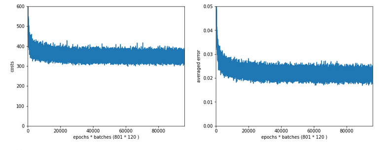
I added some statements to the method for cost calculation in order to save the relative part of the regularization terms with respect to the total costs of each mini-batch in a Numpy array and plot the evolution in the end. The changes are so simple that I omit showing the modified code.
A first look at the evolution of the relative contribution of regularization to the total loss of a mini-batch
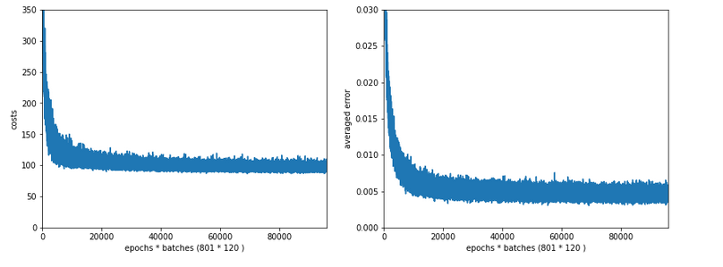
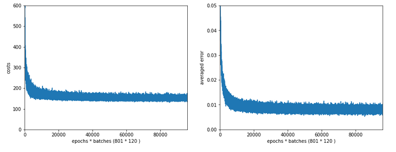
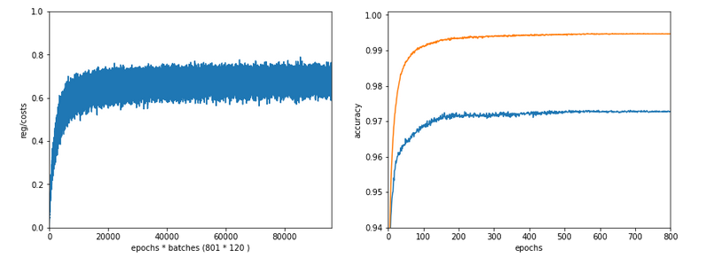
How does the outcome of gradient descent look for standardized input data and a Lambda2-value of 0.1?
Lambda2 = 0.1
Results: acc_train: 0.999 , acc_test: 0.9714, convergence after ca. 600 epochs
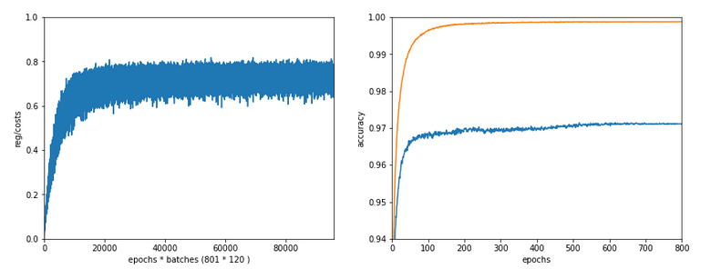
We see that the regularization term actually dominates the total loss of a mini-batch at convergence. At least with our present parameter setting. In comparisoin to the total loss of the full training set the contribution is of course much smaller and typically below 1%.
A small Lambda term
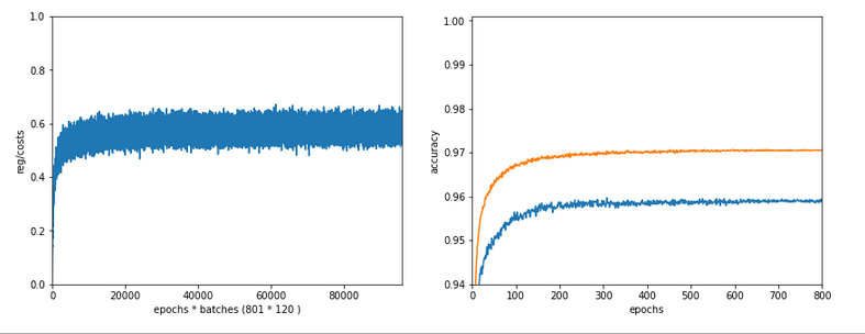
Let us reduce the regularization term via setting Lambda = 0.01. We expect its initial contribution to the costs of a batch to be smaller then, but this does NOT mean that the ratio to the standard costs of the batch automatically shrinks significantly, too:
Lambda2 = 0.01
Results: acc_train: 1.0 , acc_test: 0.9656, convergence after ca. 350 epochs
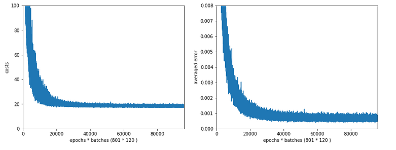
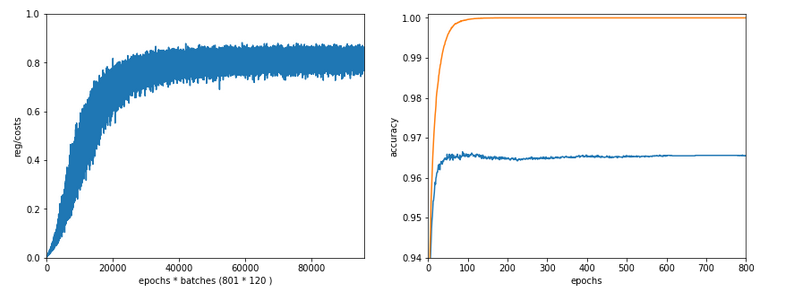
Note the absolute scale of the costs in the plots! We ended up at a much lower level of the total loss of a batch! But the relative dominance of regularization at the point of convergence actually increased! However, this did not help us with the accuracy of our MLP-algorithm on the test data set – although we perfectly fit the training set by a 100% accuracy.
In the end this is what regularization is all about. We do not want a total overfitting, a perfect adaption of the grid to the training set. It will not help in the sense of getting a better general accuracy on other input data. A Lambda2 of 0.01 is much too small in our case!
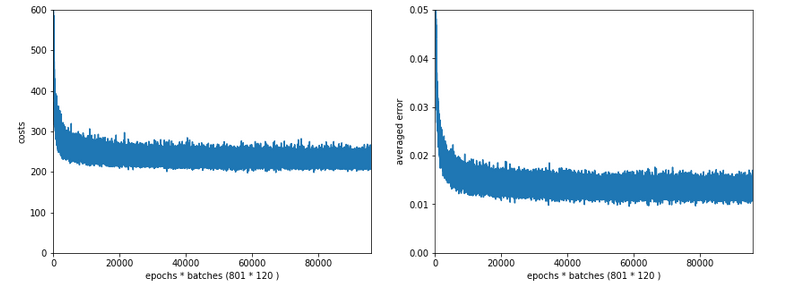
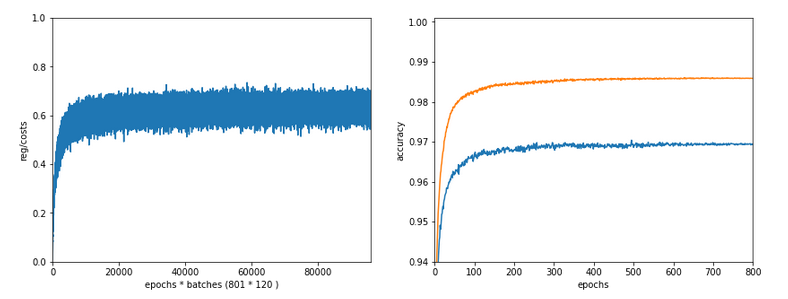
Slightly bigger regularization with Lambda2 = 0.2
So lets enlarge Lambda2 a bit:
Lambda2 = 0.2
Results: acc_train: 0.9946 , acc_test: 0.9728, convergence after ca. 700 epochs
We get an improved accuracy!
Two other cases with significantly bigger Lambda2
Lambda2 = 0.4
Results: acc_train: 0.9858 , acc_test: 0.9693, convergence after ca. 600 epochs
Lambda2 = 0.8
Results: acc_train: 0.9705 , acc_test: 0.9588, convergence after ca. 400 epochs
OK, but in both cases we see a significant and systematic trend towards reduced accuracy values on the test data set with growing Lambda2-values > 0.2 for our chosen mini-batch size (500 samples).
Conclusion
We learned a bit about the impact of regularization today. Whatever the exact Lambda2-value – in the end the contribution of a regularization term becomes a significant part of the total loss of a mini-batch when we approached the total cost minimum. However, the factor Lambda2 must be chosen with a reasonable size to get an impact of regularization on the final minimum position in the weight-space! But then it will help to improve accuracy on general input data in comparison to overfitted solutions!
But we also saw that there is some balance to take care of: For an optimum of generalization AND accuracy you should neither make Lambda2 too small nor too big. In our case Lambda2 = 0.2 seems to be a reasonable and good choice. Might be different with other datasets.
All in all studying the impact of a variation of achieved accuracy with the factor for a Ridge regularization term seems to be a good investment of time in ML projects. We shall come back to this point already in the next articles of this series.
In the next article
we shall start to work on cluster detection in the feature space of the MNIST data before using gradient descent.