I continue my series on a Python code for a simple multi-layer perceptron [MLP]. During the course of the previous articles we have built a Python class “ANN” with methods to import the MNIST data set and handle forward propagation as well as error backward propagation [EBP]. We also had a deeper look at the mathematics of gradient descent and EBP for MLP training.
A simple program for an ANN to cover the Mnist dataset – IX – First Tests
A simple program for an ANN to cover the Mnist dataset – VIII – coding Error Backward Propagation
A simple program for an ANN to cover the Mnist dataset – VII – EBP related topics and obstacles
A simple program for an ANN to cover the Mnist dataset – VI – the math behind the „error back-propagation“
A simple program for an ANN to cover the Mnist dataset – V – coding the loss function
A simple program for an ANN to cover the Mnist dataset – IV – the concept of a cost or loss function
A simple program for an ANN to cover the Mnist dataset – III – forward propagation
A simple program for an ANN to cover the Mnist dataset – II – initial random weight values
A simple program for an ANN to cover the Mnist dataset – I – a starting point
The code modifications in the last article enabled us to perform a first test on the MNIST dataset. This test gave us some confidence in our training algorithm: It seemed to converge and produce weights which did a relatively good job on analyzing the MNIST images.
We saw a slight tendency of overfitting. But an accuracy level of 96.5% on the test dataset showed that the MLP had indeed “learned” something during training. We needed around 1000 epochs to come to this point.
However, there are a lot of parameters controlling our grid structure and the learning behavior. Such parameters are often called “hyper-parameters“. To get a better understanding of our MLP we must start playing around with such parameters. In this article we shall concentrate on the parameter for (regression) regularization (called Lambda2 in the parameter interface of our class ANN) and then start varying the node numbers on the layers.
But before we start new test runs we add a statistical element to the training – namely the variation of the composition of our mini-batches (see the last article).
General hint: In all of the test runs below we used 4 CPU cores with libOpenBlas on a Linux system with an I7 6700K CPU.
Shuffling the contents of the mini-batches
Let us add some more parameters to the interface of class “ANN”:
shuffle_batches = True
print_period = 20
The first parameter
shall control whether we vary the composition of the mini-batches with each epoch. The second parameter controls for which period of the epochs we print out some intermediate data (costs, averaged error of last mini-batch).
    def __init__(self,
                 my_data_set = "mnist",
                 n_hidden_layers = 1,
                 ay_nodes_layers = [0, 100, 0], # array which should have as much elements as n_hidden + 2
                 n_nodes_layer_out = 10,  # expected number of nodes in output layer

                 my_activation_function = "sigmoid",
                 my_out_function        = "sigmoid",
                 my_loss_function       = "LogLoss",

                 n_size_mini_batch = 50,  # number of data elements in a mini-batch

                 n_epochs      = 1,
                 n_max_batches = -1,  # number of mini-batches to use during epochs - > 0 only for testing
                                      # a negative value uses all mini-batches

                 lambda2_reg = 0.1,     # factor for quadratic regularization term
                 lambda1_reg = 0.0,     # factor for linear regularization term

                 vect_mode = 'cols',

                 learn_rate = 0.001,        # the learning rate (often called epsilon in textbooks)
                 decrease_const = 0.00001,  # a factor for decreasing the learning rate with epochs
                 mom_rate   = 0.0005,       # a factor for momentum learning

                 shuffle_batches = True,    # True: we mix the data for mini-batches in the X-train set at the start of each epoch

                 print_period = 20,         # number of epochs for which to print the costs and the averaged error

                 figs_x1=12.0, figs_x2=8.0,
                 legend_loc='upper right',

                 b_print_test_data = True

                 ):
        '''
        Initialization of MyANN
        Input:
            data_set: type of dataset; so far only the "mnist", "mnist_784" datsets are known
                      We use this information to prepare the input data and learn about the feature dimension.
                      This info is used in preparing the size of the input layer.
            n_hidden_layers = number of hidden layers => between input layer 0 and output layer n

            ay_nodes_layers = [0, 100, 0 ] : We set the number of nodes in input layer_0 and the output_layer to zero
                              Will be set to real number afterwards by infos from the input dataset.
                              All other numbers are used for the node numbers of the hidden layers.
            n_nodes_out_layer = expected number of nodes in the output layer (is checked);
                                this number corresponds to the number of categories NC = number of labels to be distinguished

            my_activation_function : name of the activation function to use
            my_out_function : name of the "activation" function of the last layer which produces the output values
            my_loss_function : name of the "cost" or "loss" function used for optimization

            n_size_mini_batch : Number of elements/samples in a mini-batch of training data
                                The number of mini-batches will be calculated from this

            n_epochs : number of epochs to calculate during training
            n_max_batches : > 0: maximum of mini-batches to use during training

      < 0: use all mini-batches

            lambda_reg2:    The factor for the quadartic regularization term
            lambda_reg1:    The factor for the linear regularization term

            vect_mode: Are 1-dim data arrays (vctors) ordered by columns or rows ?

            learn rate :     Learning rate - definies by how much we correct weights in the indicated direction of the gradient on the cost hyperplane.
            decrease_const:  Controls a systematic decrease of the learning rate with epoch number
            mom_const:       Momentum rate. Controls a mixture of the last with the present weight corrections (momentum learning)

            shuffle_batches: True => vary composition of mini-batches with each epoch

            print_period:    number of periods between printing out some intermediate data
                             on costs and the averaged error of the last mini-batch


            figs_x1=12.0, figs_x2=8.0 : Standard sizing of plots ,
            legend_loc='upper right': Position of legends in the plots

            b_print_test_data: Boolean variable to control the print out of some tests data

         '''

        # Array (Python list) of known input data sets
        self._input_data_sets = ["mnist", "mnist_784", "mnist_keras"]
        self._my_data_set = my_data_set

        # X, y, X_train, y_train, X_test, y_test
            # will be set by analyze_input_data
            # X: Input array (2D) - at present status of MNIST image data, only.
            # y: result (=classification data) [digits represent categories in the case of Mnist]
        self._X       = None
        self._X_train = None
        self._X_test  = None
        self._y       = None
        self._y_train = None
        self._y_test  = None

        # relevant dimensions
        # from input data information;  will be set in handle_input_data()
        self._dim_sets     = 0
        self._dim_features = 0
        self._n_labels     = 0   # number of unique labels - will be extracted from y-data

        # Img sizes
        self._dim_img      = 0 # should be sqrt(dim_features) - we assume square like images
        self._img_h        = 0
        self._img_w        = 0

        # Layers
        # ------
        # number of hidden layers
        self._n_hidden_layers = n_hidden_layers
        # Number of total layers
        self._n_total_layers = 2 + self._n_hidden_layers
        # Nodes for hidden layers
        self._ay_nodes_layers = np.array(ay_nodes_layers)
        # Number of nodes in output layer - will be checked against information from target arrays
        self._n_nodes_layer_out = n_nodes_layer_out

        # Weights
        # --------
        # empty List for all weight-matrices for all layer-connections
        # Numbering :
        # w[0] contains the weight matrix which connects layer 0 (input layer ) to hidden layer 1
        # w[1] contains the weight matrix which connects layer 1 (input layer ) to (hidden?) layer 2
        self._li_w = []

        # Arrays for encoded output labels - will be set in _encode_all_mnist_labels()
        # -------------------------------
        self._ay_onehot = None
        self._ay_oneval = None

        # Known Randomizer methods ( 0: np.random.randint, 1: np.random.uniform )
        # ------------------
        self.__ay_known_randomizers = [0, 1]

        # Types of activation functions and output functions
        # ------------------
        self.__ay_activation_functions = ["sigmoid"] # later also relu
        self.__ay_output_functions     = ["sigmoid"] # later also
softmax

        # Types of cost functions
        # ------------------
        self.__ay_loss_functions = ["LogLoss", "MSE" ] # later also other types of cost/loss functions


        # the following dictionaries will be used for indirect function calls
        self.__d_activation_funcs = {
            'sigmoid': self._sigmoid,
            'relu':    self._relu
            }
        self.__d_output_funcs = {
            'sigmoid': self._sigmoid,
            'softmax': self._softmax
            }
        self.__d_loss_funcs = {
            'LogLoss': self._loss_LogLoss,
            'MSE': self._loss_MSE
            }
        # Derivative functions
        self.__d_D_activation_funcs = {
            'sigmoid': self._D_sigmoid,
            'relu':    self._D_relu
            }
        self.__d_D_output_funcs = {
            'sigmoid': self._D_sigmoid,
            'softmax': self._D_softmax
            }
        self.__d_D_loss_funcs = {
            'LogLoss': self._D_loss_LogLoss,
            'MSE': self._D_loss_MSE
            }


        # The following variables will later be set by _check_and set_activation_and_out_functions()

        self._my_act_func  = my_activation_function
        self._my_out_func  = my_out_function
        self._my_loss_func = my_loss_function
        self._act_func = None
        self._out_func = None
        self._loss_func = None

        # number of data samples in a mini-batch
        self._n_size_mini_batch = n_size_mini_batch
        self._n_mini_batches = None  # will be determined by _get_number_of_mini_batches()

        # maximum number of epochs - we set this number to an assumed maximum
        # - as we shall build a backup and reload functionality for training, this should not be a major problem
        self._n_epochs = n_epochs

        # maximum number of batches to handle ( if < 0 => all!)
        self._n_max_batches = n_max_batches
        # actual number of batches
        self._n_batches = None

        # regularization parameters
        self._lambda2_reg = lambda2_reg
        self._lambda1_reg = lambda1_reg

        # parameter for momentum learning
        self._learn_rate = learn_rate
        self._decrease_const = decrease_const
        self._mom_rate   = mom_rate
        self._li_mom = [None] *  self._n_total_layers

        # shuffle data in X_train?
        self._shuffle_batches = shuffle_batches

        # epoch period for printing
        self._print_period = print_period

        # book-keeping for epochs and mini-batches
        # -------------------------------
        # range for epochs - will be set by _prepare-epochs_and_batches()
        self._rg_idx_epochs = None
        # range for mini-batches
        self._rg_idx_batches = None
        # dimension of the numpy arrays for book-keeping - will be set in _prepare_epochs_and_batches()
        self._shape_epochs_batches = None    # (n_epochs, n_batches, 1)

        # list for error values at outermost layer for minibatches and epochs during training
        # we use a numpy array here because we can redimension it
        self._ay_theta = None
        # list for cost values of mini-batches during training
        # The list will later be split into sections for epochs
        self._ay_costs = None


        # Data elements for back propagation
        # ----------------------------------

        # 2-dim array of partial derivatives of the elements of an additive cost function
        # The derivative is taken with respect to the output results a_j = ay_ANN_out[j]
        # The array dimensions account for nodes and sampls of a
mini_batch. The array will be set in function
        # self._initiate_bw_propagation()
        self._ay_delta_out_batch = None


        # parameter to allow printing of some test data
        self._b_print_test_data = b_print_test_data

        # Plot handling
        # --------------
        # Alternatives to resize plots
        # 1: just resize figure  2: resize plus create subplots() [figure + axes]
        self._plot_resize_alternative = 1
        # Plot-sizing
        self._figs_x1 = figs_x1
        self._figs_x2 = figs_x2
        self._fig = None
        self._ax  = None
        # alternative 2 does resizing and (!) subplots()
        self.initiate_and_resize_plot(self._plot_resize_alternative)


        # ***********
        # operations
        # ***********

        # check and handle input data
        self._handle_input_data()
        # set the ANN structure
        self._set_ANN_structure()

        # Prepare epoch and batch-handling - sets ranges, limits num of mini-batches and initializes book-keeping arrays
        self._rg_idx_epochs, self._rg_idx_batches = self._prepare_epochs_and_batches()

        # perform training
        start_c = time.perf_counter()
        self._fit(b_print=True, b_measure_batch_time=False)
        end_c = time.perf_counter()
        print('\n\n ------')
        print('Total training Time_CPU: ', end_c - start_c)
        print("\nStopping program regularily")
Both parameters affect our method “_fit()” in the following way :
    ''' -- Method to set the number of batches based on given batch size -- '''
    def _fit(self, b_print = False, b_measure_batch_time = False):
        '''
        Parameters:
            b_print:                 Do we print intermediate results of the training at all?
            b_print_period:          For which period of epochs do we print?
            b_measure_batch_time:    Measure CPU-Time for a batch
        '''
        rg_idx_epochs  = self._rg_idx_epochs
        rg_idx_batches = self._rg_idx_batches
        if (b_print):
            print("\nnumber of epochs = " + str(len(rg_idx_epochs)))
            print("max number of batches = " + str(len(rg_idx_batches)))

        # loop over epochs
        for idxe in rg_idx_epochs:
            if (b_print and (idxe % self._print_period == 0) ):
                print("\n ---------")
                print("\nStarting epoch " + str(idxe+1))

            # sinmple adaption of the learning rate
            self._learn_rate /= (1.0 + self._decrease_const * idxe)

            # shuffle indices for a variation of the mini-batches with each epoch
            if self._shuffle_batches:
                shuffled_index = np.random.permutation(self._dim_sets)
                self._X_train, self._y_train, self._ay_onehot = self._X_train[shuffled_index], self._y_train[shuffled_index], self._ay_onehot[:, shuffled_index]


            # loop over mini-batches
            for idxb in rg_idx_batches:
                if b_measure_batch_time:
                    start_0 = time.perf_counter()
                # deal with a mini-batch
                self._handle_mini_batch(num_batch = idxb, num_epoch=idxe, b_print_y_vals = False, b_print = False)
                if b_measure_batch_time:
                    end_0 = time.perf_counter()
                    print('Time_CPU for batch ' + str(idxb+1), end_0 - start_0)

            if (b_print and (idxe % self._print_period == 0) ):
                print("\ntotal costs of mini_batch = ", self._ay_costs[idxe, idxb])

          print("avg total error of mini_batch = ", self._ay_theta[idxe, idxb])

        return None
Results for shuffling the contents of the mini-batches
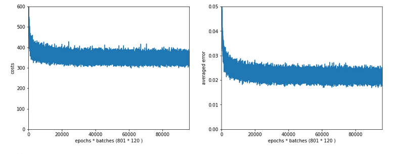
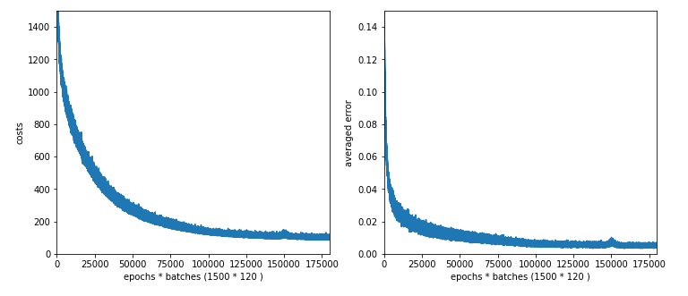
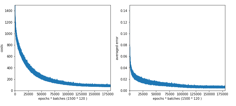
With shuffling we expect a slightly broader variation of the costs and the averaged error. But the accuracy should no change too much in the end. We start a new test run with the following parameters:
     ay_nodes_layers = [0, 70, 30, 0],
     n_nodes_layer_out = 10,
     my_loss_function = "LogLoss",
     n_size_mini_batch = 500,
     n_epochs = 1500,
     n_max_batches = 2000,  # small values only for test runs
     lambda2_reg = 0.1,
     lambda1_reg = 0.0,
     vect_mode = 'cols',
     learn_rate = 0.0001,
     decrease_const = 0.000001,
     mom_rate   = 0.00005,
     shuffle_batches = True,
     print_period = 20,
...
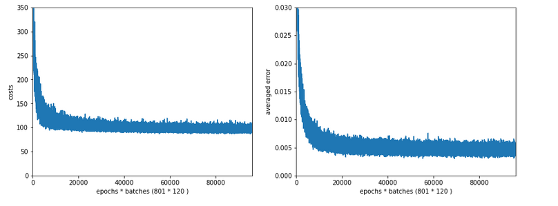
If we look at the intermediate printout for the last mini-batch of some epochs and compare it to the results given in the last article, we see a stronger variation in the costs and averaged error. The reason is that the composition of last mini-batch of an epoch changes with every epoch.
number of epochs = 1500
max number of batches = 120
---------
Starting epoch 1
total costs of mini_batch =  1757.7650929607967
avg total error of mini_batch =  0.17086198431410954
---------
Starting epoch 61
total costs of mini_batch =  511.7001121819204
avg total error of mini_batch =  0.030287362041332373
---------
Starting epoch 121
total costs of mini_batch =  435.2513093033654
avg total error of mini_batch =  0.023445601362614754
----------
Starting epoch 181
total costs of mini_batch =  361.8665831722295
avg total error of mini_batch =  0.018540003201911136
---------
Starting epoch 241
total costs of mini_batch =  293.31230634431023
avg total error of mini_batch =  0.0138237366634751
---------
Starting epoch 301
total costs of mini_batch =  332.70394217467936
avg total error of mini_batch =  0.017697548541363246
---------
Starting epoch 361
total costs of mini_batch =  249.26400606039937
avg total error of mini_batch =  0.011765164578232358
---------
Starting epoch 421
total costs of mini_batch =  240.0503762160913
avg total error of mini_batch =  0.011650843329895542
---------
Starting epoch 481
total costs of mini_batch =  222.89422430417295
avg total error of mini_batch =  0.011503859412784031
---------
Starting epoch 541
total costs of mini_batch =  200.1195962051405
avg total error of mini_batch =  0.009962020519104173
---------
tarting epoch 601
total costs of mini_batch =  206.74753168607685
avg total error of mini_batch =  0.01067995191155135
---------
Starting epoch 661
total costs of mini_batch =  171.14090717705736
avg total error of mini_batch =  0.0077091934178393105
---------
Starting epoch 721
total costs of mini_batch =  158.44967190977957
avg total error of mini_batch =  0.0070760922760890735
---------
Starting epoch 781
total costs of mini_batch =  165.4047453537401
avg total error of mini_batch =  0.008622788115637027
---------
Starting epoch 841
total costs of mini_batch =  140.52762105883642
avg total error of mini_batch =  0.0067360505574077766
---------
Starting epoch 901
total costs of mini_batch =  163.9117184790982
avg total error of mini_batch =  0.007431666926365192
---------
Starting epoch 961
total costs of mini_batch =  126.05539161877512
avg total error of mini_batch =  0.005982378079899406
---------
Starting epoch 1021
total costs of mini_batch =  114.89943308334199
avg total error of mini_batch =  0.005122976288751798
---------
Starting epoch 1081
total costs of mini_batch =  117.22051220670932
avg total error of mini_batch
=  0.005185936692097749
---------
Starting epoch 1141
total costs of mini_batch =  140.88969853048422
avg total error of mini_batch =  0.007665464508660714
---------
Starting epoch 1201
total costs of mini_batch =  113.27223303239667
avg total error of mini_batch =  0.0059791015452599705
---------
Starting epoch 1261
total costs of mini_batch =  105.55343407063131
avg total error of mini_batch =  0.005000503315756879
---------
Starting epoch 1321
total costs of mini_batch =  130.48116668827038
avg total error of mini_batch =  0.006287118265324945
---------
Starting epoch 1381
total costs of mini_batch =  109.04042315247389
avg total error of mini_batch =  0.005874339148860562
---------
Starting epoch 1441
total costs of mini_batch =  121.01379412127089
avg total error of mini_batch =  0.0065105907117289944
---------
Starting epoch 1461
total costs of mini_batch =  103.08774822996196
avg total error of mini_batch =  0.005299079778792264
---------
Starting epoch 1481
total costs of mini_batch =  106.21334182056928
avg total error of mini_batch =  0.005343967730134955
-------
Total training Time_CPU:  1963.8792177759988
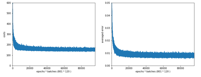
Note that the averaged error values result from averaging of the absolute values of the errors of all records in a batch! The small numbers are not due to a cancelling of positive by negative deviations. A contribution to the error at an output node is given by the absloute value of the difference between the predicted real output value and the encoded target output value. We then first calculate an average over all output nodes (=10) per record and then average these values over all records of a batch. Such an “averaged error” gives us a first indication of the accuracy level reached.
Note that this averaged error is not becoming a constant. The last values in the above list indicate that we do not get much better with the error than 0.0055 on the training data. Our approached minimum points on the various cost hyperplanes of the mini-batches obviously hop around the global minimum on the hyperplane of the total costs. One of the reasons is the varying composition of the mini-batches; another reason is that the cost hyperplanes of the various mini-batches themselves are different from the hyperplane of the total costs of all records of the test data set. We see the effects of a mixture of “batch gradient descent” and “stochastic gradient descent” here; i.e., we do not get rid of stochastic elements even if we are close to a global minimum.
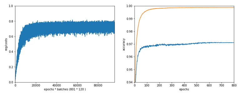
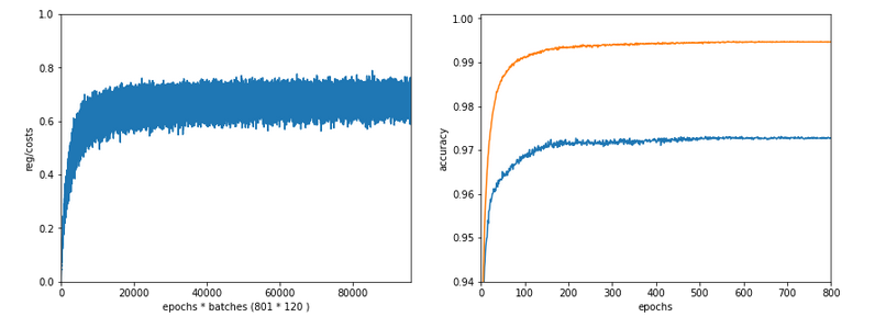
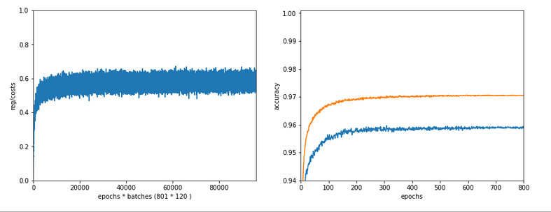
Still we observe an overall convergent behavior at around 1050 epochs. There our curves get relatively flat.
Accuracy values are:
total accuracy for training data = 0.9914
total accuracy for test data = 0.9611
So, this is pretty much the same as in our original run in the last article without data shuffling.
Dropping regularization
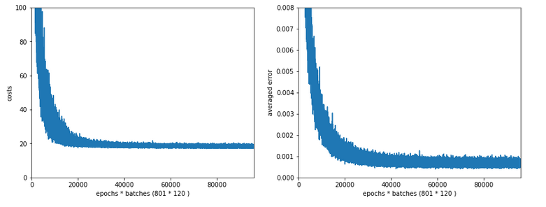
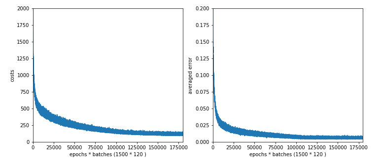
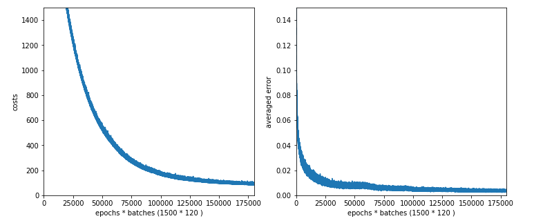
In the above run we had used a quadratic from of the regularization (often called Ridge regularization). In the next test run we shall drop regularization completely (Lambda2 = 0, Lambda1 = 0) and find out whether this hampers the generalization of our MLP and the resulting accuracy with respect to the test data set.
Resulting data for the last epochs of the test run are
Starting epoch 1001
total costs of mini_batch =  67.98542512352101
avg total error of mini_batch =  0.007449654093429594
---------
nStarting epoch 1051
total costs of mini_batch =  56.69195783294443
avg total error of mini_batch =  0.0063384571747725415
---------
Starting epoch 1101
total costs of mini_batch =  51.81035466850738
avg total error of mini_batch =  0.005939699354987233
---------
Starting epoch 1151
total costs of mini_batch =  52.23157716632318
avg total error of mini_batch =  0.006373981433882217
---------
Starting epoch 1201
total costs of mini_batch =  48.40298652277855
avg total error of mini_batch =  0.005653856253701317
---------
Starting epoch 1251
total costs of mini_batch =  45.00623540189525
avg total error of mini_batch =  0.005245339176038497
---------
Starting epoch 1301
total costs of mini_batch =  36.88409532579881
avg total error of mini_batch =  0.004600719544961844
---------
Starting epoch 1351
total costs of mini_batch =  36.53543045554845
avg total error of mini_batch =  0.003993852242709943
---------
Starting epoch 1401
total costs of mini_batch =  38.80422469954769
avg total error of mini_batch =  0.00464620714991714
---------
Starting epoch 1451
total costs of mini_batch =  42.39371261881638
avg total error of mini_batch =  0.005294796697150631
------
Total training Time_CPU:  2118.4527089519997
Note, by the way, that the absolute values of the costs depend on the regularization parameter; therefore we see somewhat lower values in the end than before. But the absolute cost values are not so important regarding the general convergence and the accuracy of the network reached.
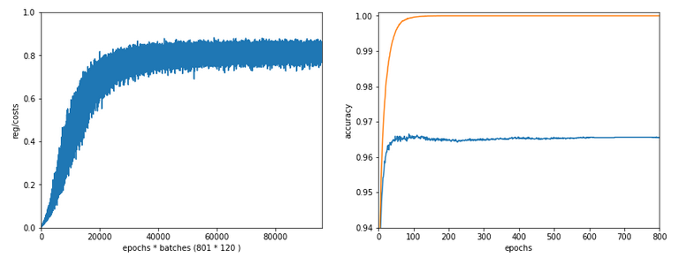
We omit the plots and just give the accuracy values:
total accuracy for training data = 0.9874
total accuracy for test data = 0.9514
We get a slight drop in accuracy for the test data set – small (1%), but notable. It is interesting the even the accuracy on the training data became influenced.
Why might it be interesting to check the impact of the regularization?
We learn from literature that regularization helps with overfitting. Another aspect discussed e.g. by Jörg Frochte in his book “Maschinelles Lernen” is, whether we have enough training data to determine the vast amount of weights in complicated networks. He suggests on page 190 of his book to consider the number of weights in an MLP and compare it with the number of available data points.
He suggests that one may run into trouble if the difference between the number of weights (number of degrees of freedom) and the number of data records (number of independent information data) becomes too big. However, his test example was a rather limited one and for regression not classification. He also notes that if the data are well distributed may not be as big as assumed. If one thinks about it, one may also come to the question whether the real amount of data provided by the records is not by a factor of 10 larger – as we use 10 output values per record ….
Anyway, I think it is worthwhile to have a look at regularization.
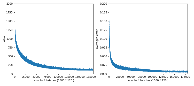
Enlarging the regularization factor
We double the value of Lambda2: Lambda2 = 0.2.
Starting epoch 1251
total costs of mini_batch =  128.00827405482318
avg total error of mini_batch =  0.007276206815511017
---------
Starting epoch 1301
total costs of mini_batch =  107.62983581797556
avg total error of mini_batch =  0.005535653858885446
---------
Starting epoch 1351
total costs of mini_batch =  107.83630092292944
avg total error of mini_batch =  0.
005446805325519184
---------
Starting epoch 1401
total costs of mini_batch =  119.7648277329852
avg total error of mini_batch =  0.00729466852297802
---------
Starting epoch 1451
total costs of mini_batch =  106.74254206278933
avg total error of mini_batch =  0.005343124456075227
We get a slight improvement of the accuracy compared to our first run with data shuffling:
total accuracy for training data = 0.9950
total accuracy for test data = 0.964
So, regularization does have its advantages. I recommend to investigate the impact of this parameter closely, if you need to get the “last percentages” in generalization and accuracy for a given MLP-model.
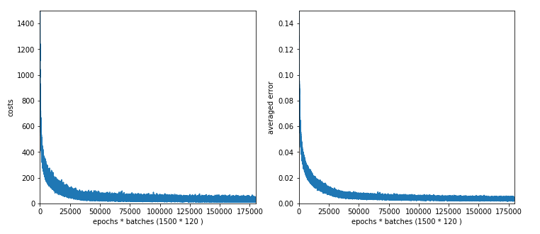
Enlarging node numbers
We have 60000 data records in the training set. In our example case we needed to fix around 784*70 + 70*30 + 30*10 = 57280 weight values. This is pretty close to the total amount of training data (60000). What happens if we extend the number of weights beyond the number of training records?
E.g. 784*100 + 100*50 + 50*10 = 83900. Do we get some trouble?
The results are:
Starting epoch 1151
total costs of mini_batch =  109.77341617599176
avg total error of mini_batch =  0.005494982077591186
---------
Starting epoch 1201
total costs of mini_batch =  113.5293680548904
avg total error of mini_batch =  0.005352117137100675
---------
Starting epoch 1251
total costs of mini_batch =  116.26371170820423
avg total error of mini_batch =  0.0072335516486698
---------
Starting epoch 1301
total costs of mini_batch =  99.7268420386945
avg total error of mini_batch =  0.004850817052601995
---------
Starting epoch 1351
total costs of mini_batch =  101.16579732551999
avg total error of mini_batch =  0.004831600835072556
---------
Starting epoch 1401
total costs of mini_batch =  98.45208584213253
avg total error of mini_batch =  0.004796133492821962
---------
Starting epoch 1451
total costs of mini_batch =  99.279344780807
avg total error of mini_batch =  0.005289728162205425
------
Total training Time_CPU:  2159.5880855739997
Ooops, there appears a glitch in the data around epoch 1250. Such things happen! So, we should have a look at the graphs before we decide to take the weights of a special epoch for our MLP model!
But in the end, i.e. with the weights at epoch 1500 the accuracy values are:
total accuracy for training data = 0.9962
total accuracy for test data = 0.9632
So, we were NOT punished by extending our network, but we gained nothing worth the effort.
Now, let us go up with node numbers much more: 300 and 100 => 784*300 + 300*100 + 100*10 = 266200; ie. substantially more individual weights than training samples! First with Lambda2 = 0.2:
Starting epoch 1201
total costs of mini_batch =  104.4420759423322
avg total error of mini_batch =  0.0037985801450468246
---------
Starting epoch 1251
total costs of mini_batch =  102.80878647657674
avg total error of mini_batch =  0.003926855904089417
---------
Starting epoch 1301
total costs of mini_batch =  100.01189950545002
avg total error of mini_batch =  0.0037743225368465773
---------
Starting epoch 1351
total
costs of mini_batch =  97.34294880936079
avg total error of mini_batch =  0.0035513092392408865
---------
Starting epoch 1401
total costs of mini_batch =  93.15432903284587
avg total error of mini_batch =  0.0032916082743134206
---------
Starting epoch 1451
total costs of mini_batch =  89.79127326241868
avg total error of mini_batch =  0.0033628384147655283
------
Total training Time_CPU:  4254.479082876998
total accuracy for training data = 0.9987
total accuracy for test data = 0.9630
So , much CPU-time for no gain!
Now, what happens if we set Lambda2 = 0? We get:
total accuracy for training data = 0.9955
total accuracy for test data = 0.9491
This is a small change around 1.4%! I would say:
In the special case of MNIST, a MLP-network with 2 hidden layers and a small learning rate we see neither a major problem regarding the amount of available data, nor a dramatic impact of the regularization. Regularization brings around a 1% gain in accuracy.
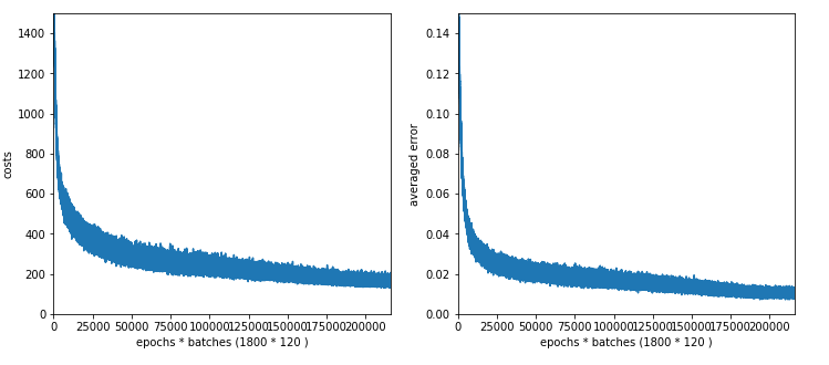
Reducing the node number on the hidden layers
Another experiment could be to reduce the number of nodes on the hidden layers. Let us go down to 40 nodes on L1 and 20 on L2, then to 30 and 20. Lambda2 is set to 0.2 in both runs. acc1 in the following listing means the accuracy for the training data, acc2 for the test data.
The results are:
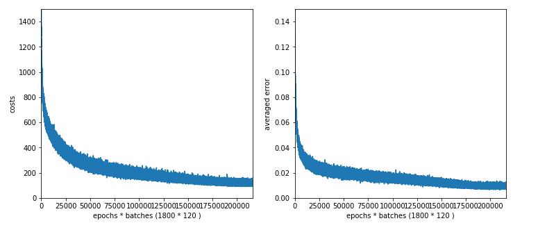
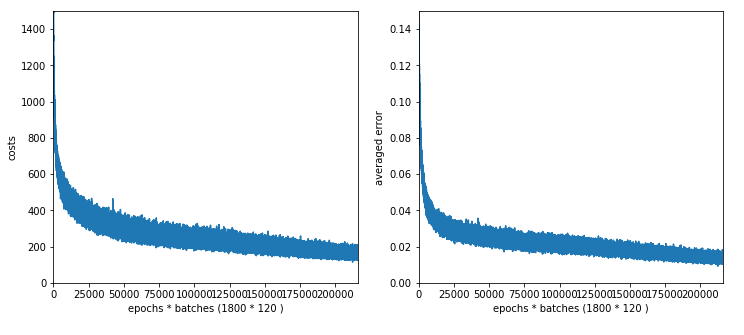
40 nodes on L1, 20 nodes on L2, 1500 epochs => 1600 sec, acc1 = 0.9898, acc2 = 0.9578
30 nodes on L1, 20 nodes on L2, 1800 epochs => 1864 sec, acc1 = 0.9861, acc2 = 0.9513
We loose around 1% in accuracy!
The plot for 30, 20 nodes on layers L1, L2 shows that we got a convergence only beyond 1500 epochs.
Working with just one hidden layer
To get some more indications regarding efficiency let us now turn to networks with just one layer.
We investigate three situations with the following node numbers on the hidden layer: 100, 50, 30
The plot for 100 nodes on the hidden layer; we get convergence at around 1050 epochs.
Interestingly the CPU time for 100 nodes is with 1850 secs not smaller than for the network with 70 and 30 nodes on the hidden layers. As the dominant matrices are the ones connecting layer L0 and layer L1 this is quite understandable. (Note the CPU time also depends on the consumption of other jobs on the system.
The plots for 50 and 30 nodes on the hidden layer; we get convergence at around 1450 epochs. The
CPU time for 1500 epochs goes down to 1500 sec and XXX sec, respectively.
Plot for 50 nodes on the hidden layer:
Plot for 30 nodes:
We get the following accuracy values:
100 nodes, 1950 sec (1500 epochs), acc1 = 0.9947, acc2 = 0.9619,
50 nodes, 1600 sec (1500 epochs), acc1 = 0.9880, acc2 = 0.9566,
30 nodes, 1450 sec (1500 epochs), acc1 = 0.9780, acc2 = 0.9436
Well, now we see a drop in the accuracy by around 2% compared to our best cases. You have to decide yourself whether the gain in CPU time is worth it.
Note, by the way, that the accuracy value for 50 nodes is pretty close to the value S. Rashka got in his book “Python Machine Learning”. If you compare such values with your own runs be aware of the rather small learning rate (0.0001) and momentum rates (0.00005) I used. You can probably become faster with smaller learning rates. But then you may need another type of adaption for the learning rate compared to our simple linear one.
Conclusion
We saw that our original guess of a network with 2 hidden layers with 70 and 30 nodes was not a bad one. A network with just one layer with just 50 nodes or below does not give us the same accuracy. However, we neither saw a major improvement if we went to grids with 300 nodes on layer L1 and 100 nodes on layer L2. Despite some discrepancy between the number of weights in comparison to the number of test records we saw no significant loss in accuracy either – with or without regularization.
We also learned that we should use regularization (here of the quadratic type) to get the last 1% to 2% bit of accuracy on the test data in our special MNIST case.
In the next article
A simple program for an ANN to cover the Mnist dataset – XI – confusion matrix
we shall have a closer look at those MNIST number images where our MLP got problems.