Multivariate Normal Distributions – II – random vectors and their covariance matrix

This post requires Javascript to display formulas!

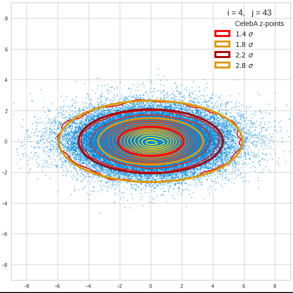
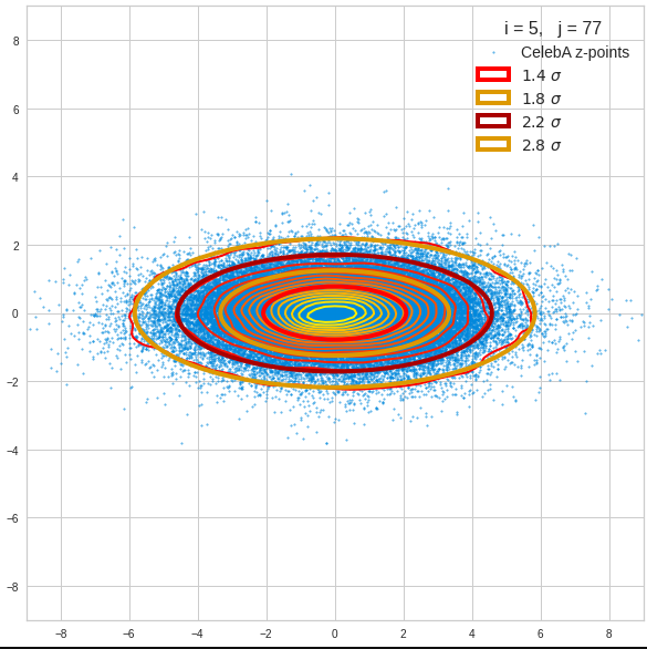
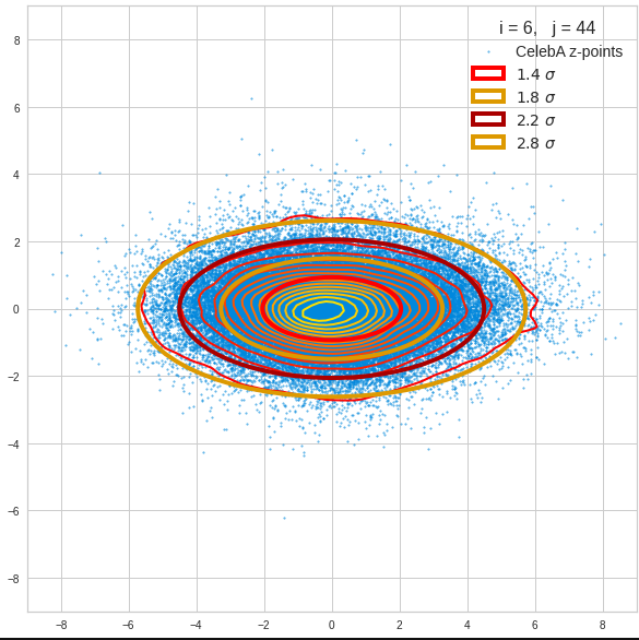
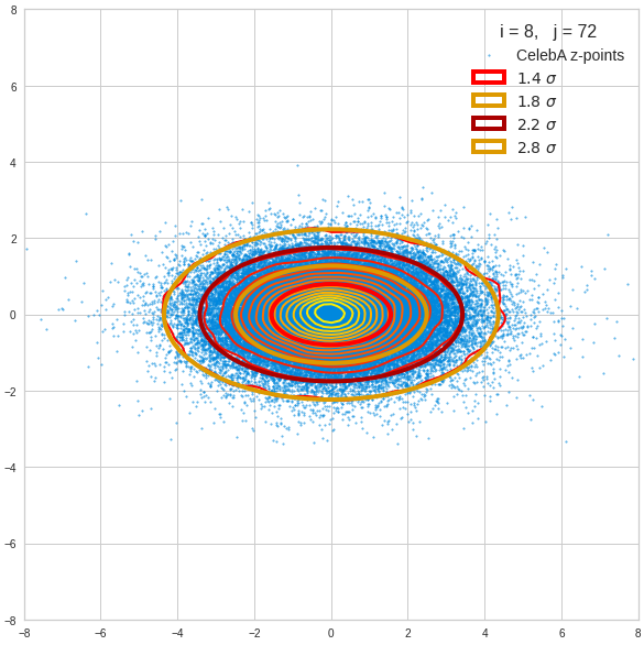
This post series is based on notes I took when I recently studied the mathematical properties of Multivariate Normal Distributions [MNDs]. A motivation to publish the notes came from the analysis of a Machine Learning experiment: A Convolutional Autoencoder [CAE] trained on human face images had produced a MND in its latent space. But MNDs are, of course, relevant in other contexts, too.

In this post we take some preparatory steps: I want to introduce the term “random vector” to describe statistical multivariate distributions in vector form. We then have a look at the definition of a probability density function [pdf] in multiple dimensions. Furthermore we discuss linear transformations of a random vector, its expectation values and its covariance matrix. The latter both marks and quantifies (linear) relations between its components. I will also point out a simple but useful equation for the behavior of the covariance matrix when a matrix operates on its random vector. Eventually we also have a look at marginal distributions and their probability density function.

I will proceed not too formally and my discussion of the topics will not be really complete in a pure mathematical sense. On our way I will also remind you of some basic ideas and equations from statistics. People who are familiar with all the terms named above can jump over this post.

Random Vectors and multivariate distributions

Let us assume that we can describe an object of interest, e.g. in the context of an ML problem, by a set of n indexed, real-value variables sj. Instead of a manifest object we could also use n variables to characterize the result of a well defined experiment. When I speak of “objects below I include this more abstract option.

Each object can mathematically be represented by a data point in the ℝn. We simply relate each of the indexed coordinate axes of a corresponding Euclidean coordinate system with a certain object property. The coordinates of the data points are then given by the variable values.

Let us now order a complete set of parallel measured property values sjc for a concrete object as indexed components of a vector sc. The vector then represents our object:

\[ \pmb{s}^c \: = \: \left( \, s_1^c, \, s_2^c, \, ….\, s_n^c\, \right)^T \,
\]

The T indicates the transposition operation. Note: Throughout this post series we assume that untransposed vectors are written in vertical form. I.e. the components are arranged as rows.

Samples

Let us assume that we have m concrete observations of individual objects (or experimental results). The values of the n real variables for each object are always measured or qualified in parallel:

  • We either randomly pick a bunch of m concrete objects out of a wider population of available objects and determine the values of their n characteristic sj-variables.
  • Or we repeat a concrete experiment, whose outcome is described by values for a set of n measurable sj-variables, many times. The setup for our experiment defines precisely what the variables are and how we measure their values. The experimental result can be interpreted as an abstract “object”.

Thus we get samples of object data. Our experimental setup and the properties of our objects define a sample space Ω we have a clear description of how we produce one or multiple vectors s. A particular observation maps Ω to an individual vector.

Let us assume that at least in principle our vector components can take any real value. Producing a vector s can then formally be regarded as a function to ℝ:

FS: Ω   =>   ℝn,     s = FS(Ω, experiment number, … ).

A sequence of many observations, i.e. creating a sample, formally corresponds to a sequence of many independent applications of this function. An implicit (and sometime problematic) assumption is that picking multiple objects or our experiments do not influence Ω and the statistics of the basic population.

The outcome, namely a set of resulting s-vectors, depends on the statistical properties of the underlying object population. We index the k-th vector by sk.

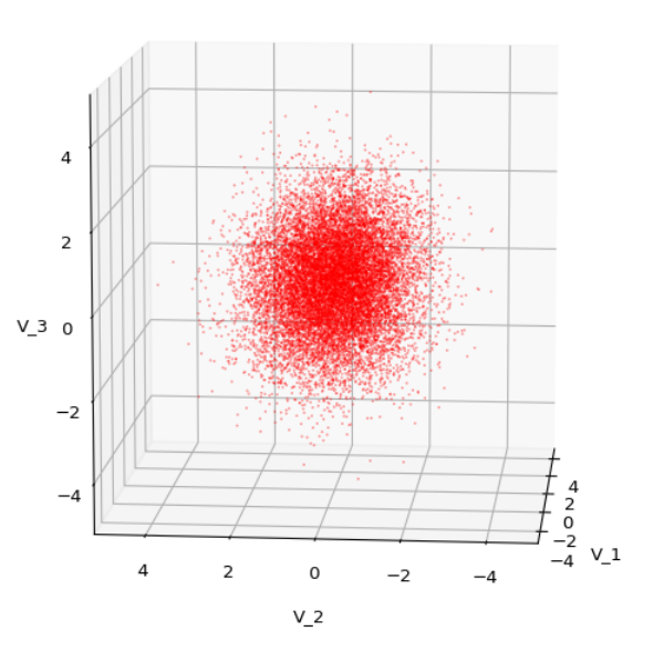
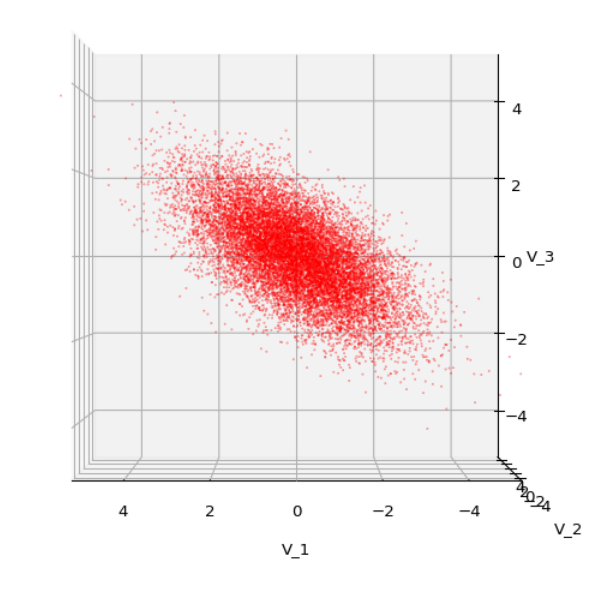
Each sample can be visualized by a bunch of data points in an n-dimensional space. A concrete sample in 3 dimensions may e.g. look like this from two perspectives:

But our sample can also be represented by a data matrix. We can e.g. arrange the columns to be given by the sk vectors. If we have a sample of m objects then we get a (n x m)- data matrix MS ∈ ℝnxm. A row with index j then provides us with a sample statistics for the j-th object property.

\[
\pmb{\operatorname{D}}_S \: = \: \begin{pmatrix}
s^1_1 & s^2_1 &\cdots & s^m_1 \\
s^1_2 & s^2_2 &\cdots & s^m_2 \\
\vdots &\vdots &\ddots &\vdots \\
s^1_n & s^2_n &\cdots & s^m_n \end{pmatrix}
\]
\[ \pmb{\operatorname{D}}_S \: = \: \left(\, \pmb{s}^1, \pmb{s}^2, \cdots …, \pmb{s}^m\right).
\]

Often you will find the transposed matrix for reasons of an efficient notation. I prefer this version as it later allows for matrix operations on the vector components from the left side, e.g. in a Python program.

Random vectors

We indicate the statistical element in creating a concrete vector from an underpinning population by a vector symbol S. By using this symbol we understand implicitly that any concrete vector S = sc is created by applying our well defined function FS.

It is natural to split S up into n individual univariate random variables Sj: Ω => ℝ, which represent the statistics per vector component. We write S in vector form:

\[ \pmb{S} \: = \: \left( \, S_1, \, S_2, \, ….\, S_n\, \right)^T
\]

So:

\[ \pmb{S} \:=\: \pmb{s}^c\: =: \left(\, S_1=s_1, S_2=s_2, \cdots …, S_n=s_n \, \right)^T.
\]

The vector variable S gets concrete component values by a well defined statistical process. But, if you like to see it more globally, S represents any object from the population and thus in a certain meaning the whole population – and its statistics.

We call S a multivariate random variable or a random vector.

Thus, our statistical multivariate distribution can now be represented by a random vector – and we know how to create samples by turning S repeatedly into concrete vectors. Why all the fuss?

Linear operations on random vectors

The vector notation allows us to combine a random vector with mathematical vector operations, in particular linear transformations. We implicitly understand that such an operation is applied to any vector of the population (and in certain contexts also to elements of our samples). Such a transformation consists of a mapping of vectors of the original population or a sample to new vectors in the same or a different vector space by one and the same linear transformation. The mapping gives us new component values.

In linear algebra we learn that a linear vector transformation can be represented by a matrix plus a translation vector. If the transformation maps a random vector S of the ℝm to a random vector X into the ℝn then the linear (affine) transformation is defined by a (n x m)-matrix A ∈ ℝnxm and a vector b ∈ ℝn:

\[ \begin{align}
\pmb{x} \,&=\, (x_1, x_2, …, x_n)^T \,=\, \pmb{\operatorname{A}} \pmb{s} \, + \, \pmb{b} \\
&\, \\
\pmb{X} \, &= \, \pmb{\operatorname{A}S} + \pmb{b} \end{align}
\]

In close similarity to standard operations in vector spaces a linear transformation of a random vector can have two meanings:

  • The operation either actively transforms our random vector (and the underlying vector distribution) – e.g. by a rotation in the ℝn.
  • Or we perform a passive switch to another Euclidean coordinate system (e.g. by a rotation of the coordinate axes) and the transformation adapts the component values accordingly.

Invertible transformations?

If and when we have a transformation within the ℝn the matrix A would typically be a real valued quadratic (n x n)-matrix. In many cases we will assume that the transformation and its matrix A are invertible. This imposes certain conditions on the matrix: A must then be positive definite and have a determinant det(A) ≠ 0.

\[ \operatorname{det}\left(\pmb{\operatorname{A}}\right) \, =\, \left|\pmb{\operatorname{A}}\right|
\, \ne \, 0
\]

But note that in the more general case also rectangular matrices can have a “left”- or a “right”-inverse matrices; see https://en.wikipedia.org/ wiki/ Generalized_ inverse.

Rectangular matrices, e.g. with m (< n) rows and n columns have a rank rm < n, and not all of the column vectors of the matrix are linearly independent.

Probability density functions in the ℝn

Let us assume that the population behind a random vector covers the ℝn completely and in a continuous way. By “continuous” we mean that a transition to infinitesimal small volumes at any position in the ℝn is possible: We still will find vectors of the population there and component values change smoothly between adjacent elements.

We can apply a frequency analysis to the vector component values of the objects of a huge sample or of a number of samples. E.g. we can define intervals into which the components may fall or not. The analysis gives us a probability P(S=sΔV) for the occurrence of position vectors sΔV which point into a certain finite region ΔV of the ℝn.

If you better like to think in terms of data points:

We get a probability that a data point representing a statistically picked object lies within a certain defined and finite region of the ℝn.

How we split up the ℝn into separate volume regions depends on available information about the object population or on an analysis of sufficiently large samples.

If each component of the vectors s can take any real value we may under certain circumstances make a transition to probability densities. Probability densities can be distilled from huge samples or alternatively very many samples picked from the underlying population. To get an idea of the density function we, in practice, raise the number of observations and reduce the volume regions of the ℝn to a proper averaging size that avoids wild fluctuations. The latter is called “sampling”.

If we by many experiments can assume a converging limiting process to infinitesimal real value intervals dsj for each of the vector components then we end up with a bunch of n continuous 1-dim probability density functions pj(sj): ℝ => ℝ. A concrete probability value for a component must be derived via integration of pj() over a finite interval a ≤ s_j ≤ b:

\[ \operatorname{P}(a \le s_j \le b) \,=\, \int_a^b p(s_j)ds_j
\]

An interpretation as a probability requires, of course, a normalization of such an integral over the whole ℝ.

It is clear that the full probability density function pS(s) of the vector distribution varies continuously with the 1-dim probability density functions of its components.

In this post series we are interested in examples of vector distributions which can be described by a continuous multidimensional probability density function [p.d.f] for infinitesimal volume elements dVS = ds1, ds2dsn:

\[ p_{\pmb{S}}(\pmb{s}) \: = \: p_{\pmb{S}} \left( \, s_1, \, s_2, \, ….\, s_n\, \right)
\]
\[ \begin{align} P(\pmb{s}, V) \, &= \, \int_V p_{\pmb{S}}(\pmb{s}) \, ds_1ds_2…ds_n \\
&= \, \int\int…\int_V p_{\pmb{S}} \left( \, s_1, \, s_2, \, ….\, s_n\, \right) \, ds_1ds_2 \cdots ds_n
\end{align}
\]

where V marks some finite volume element in ℝn. Note again: A normalization of such an integral over the whole ℝn is required to get well defined probability values. The normalization factor above is assumed to be integrated in the mathematical expression for pS(s).

For the purposes of this post series we assume that both pS and the pj() are differentiable.

Correlations of random vector components

There may be dependencies which control how the components of a random vector vary together. So the variation of pS(s) may depend in a rather complicated way on the density functions of their components pj(sj)

\[ p_{\pmb{S}}(\pmb{s}) \: = \: p_{\pmb{S}} \left( \, p_1(s_1), \, p_2(s_2), \, ….\, p_n(s_n) \, \right)
\]

The variation of components may e.g. happen in pairwise correlated or uncorrelated ways. I.e. we can in general not assume that the total probability density function pS(s) for a random vector is e.g. a product of the 1-dimensional density probability functions pj(sj for its components.

Such dependencies make the statistics of multivariate vector distributions more complex than the statistics of their constituting (marginal) univariate components. The relation between pS and the individual pj can be difficult to derive and it may even reflect non-linear component relations. Luckily we will see that MNDs contain only linear couplings of the components and thus simple correlations described by constant coefficients.

In ML we have only samples with a limited number of individual vectors available. The investigated samples have to be big enough to reveal the properties of the total probability density function pS(s), which assumedly describes the variation of the underlying continuous vector population in the ℝn.

Probability density after linear transformations and contour hyper-surfaces

A transformation of the components of a random vector has, of course, also an impact on the resulting probability density:

\[ p_{\pmb{X}}(\pmb{x}) \,=\, p_{\pmb{X}} \left( \pmb{\operatorname{A}s} \,+\, \pmb{b} \right) \, = \, p_{\pmb{X}} \left(\, x_1, \, x_2, \, ….\, x_n\, \right)
\]

and for a finite volume VX in the target space

\[ P\left(\pmb{x}, V_X\right) \,=\, \int\int…\int_{V_X} \, = \, p_{\pmb{X}} \left( x_1, \, x_2, \, ….\, x_n \right)\, dx_1dx_2 \cdots dx_n
\]

In case of a well defined distribution S we can hope to find an analytical expression for the multidimensional probability pX(x) of the transformed random vector X. But as we will see we have to invest some work into the calculation. And we will answer the question by what parameters the probability density of a MND is defined in a unique way.

We expect that the concrete form of pX is influenced in a characteristic way by the properties of the original pj(sj)-pdfs and, of course, by our transformation matrix A. This is the case for MNDs and we will study the effects of linear transformations on MNDs and their projections to sub-spaces in more detail in forthcoming posts.

As the matrix A mixes components we may also expect the creation of (linear) relations between the X-components. Therefore, the shape of the density distribution may change due to scaling, mirroring, shearing and rotation effects. This results from the fact that linear transformations are affine transformations in geometrical terms.

This leads to the question by what method we can describe the “shape” of a multivariate distribution. A simple method is to determine hyper-surfaces of constant probability density values. I.e. contour-surfaces:

\[ p_{\pmb{X}}(\pmb{x}) \, = \, p_{\pmb{X}} \left(\, x_1, \, x_2, \, ….\, x_n\, \right) \:=\: const.
\]

This actually is the definition of a (n-1)-dimensional hypersurface. The dependency on the component values can be complicated. But for the special case of a MND we will find a rather comprehensible form which we can interpret. So we will get a chance to understand and qualify the effects of a linear transformation by its impact on the contour hyper-surfaces of the probability density of a MND.

Expectation value and covariance of a statistical vector distribution

The covariance of two univariate distributions X and Y is defined as

\[
\begin{align}
\operatorname{cov}(X, Y)
&= \operatorname{\mathbb{E}}\left[\,\left(\,X \,-\, \operatorname{\mathbb{E}}\left(X\right)\,\right) \, \left(\,Y \,-\, \operatorname{\mathbb{E}}\left(Y\right)\, \right)\,\right] \\
&= \operatorname{\mathbb{E}}\left(X Y\right) \,-\, \operatorname{\mathbb{E}}\left(X\right) \operatorname{\mathbb{E}}\left(Y\right)
\end{align}
\]

The expectation value and the covariance of a general vector distribution S are defined by:

\[ \begin{align} \pmb{\mu}\left(\pmb{S}\right) \,=\, \pmb{\mu}_S \: &= \: \operatorname{\mathbb{E}}\left(\pmb{S} \right) \, := \, \left( \operatorname{\mathbb{E}}(S_1), \, \operatorname{\mathbb{E}}(S_2), …, \, \operatorname{\mathbb{E}}(S_n) \right)^T \\
\operatorname{Cov}\left(\pmb{S}\right) \: &:= \: \operatorname{\mathbb{E}}\left[\left(\pmb{S} – \operatorname{\mathbb{E}}(\pmb{S}) \right)\, \left(\pmb{S} – \operatorname{\mathbb{E}}(\pmb{S}) \right)^T \right] \end{align}
\]

Note the order of transposition in the definition of Cov! A (vertical) vector is combined with a transposed (horizontal) vector. The rules of a matrix-multiplication then give you a matrix as the result! And the expectation value has to be taken for every element of the matrix.

Thus, the interpretation of the notation given above is:

Pick all pairwise combinations (Sj, Sk) of the component distributions. Calculate the covariance of the pair cov(S_j, S_k) and put it at the (j,k)-place of the matrix.

Meaning:

\[ \begin{align}
\operatorname{Cov}\left(\pmb{S}\right)\:&=\:\operatorname{\mathbb{E}} {\begin{pmatrix} (S_{1}-\mu_{1})^{2}&(S_{1}-\mu_{1})(S_{2}-\mu_{2})&\cdots &(S_{1}-\mu_{1})(S_{n}-\mu_{n})\\(S_{2}-\mu_{2})(S_{1}-\mu_{1})&(S_{2}-\mu_{2})^{2}&\cdots &(S_{2}-\mu _{2})(S_{n}-\mu_{n})\\\vdots &\vdots &\ddots &\vdots \\(S_{n}-\mu_{n})(S_{1}-\mu_{1})&(S_{n}-\mu_{n})(S_{2}-\mu _{2})&\cdots &(X_{n}-\mu_{n})^{2} \end{pmatrix}}
\\\\
&=\quad {\begin{pmatrix} \operatorname{Var} (S_{1})&\operatorname{Cov} (S_{1},S_{2})&\cdots &\operatorname{Cov} (S_{1},S_{n})\\ \operatorname{Cov} (S_{2},S_{1})&\operatorname{Var} (S_{2})&\cdots &\operatorname{Cov} (S_{2},S_{n})\\\vdots &\vdots &\ddots &\vdots \\ \operatorname{Cov} (S_{n},S_{1})&\operatorname{Cov} (S_{n},S_{2})&\cdots &\operatorname {Var} (S_{n}) \end{pmatrix}}
\end{align}
\]

Keep the details of this definition in mind!

The above matrix is the (variance-) covariance matrix. As Wikipedia tells you, some people call it a bit different. I refer to it later on just as the covariance matrix (of a random vector).

Useful properties of the covariance matrix of a random vector

Note that the diagonal elements of the covariance matrix are just the variances of the individual component distributions, whilst the off diagonal elements contain the pairwise covariances of the vector components. In case of a vector distribution with uncorrelated (or even independent) Sj the matrix becomes diagonal:

\[
\begin{pmatrix}
(\sigma_1^s)^2 & 0 &\cdots & 0 \\
0 & (\sigma_2^s)^2 &\cdots & 0 \\
\vdots &\vdots &\ddots &\vdots \\
0 & 0 &\cdots & (\sigma_n^s)^2 \end{pmatrix}
\]


Other properties can be derived from the linearity of expectation values and the fact that

\[ \begin{align} \operatorname{Cov}\left(aX+bY,\,cW+dV\right) \,=\, ac*\operatorname{Cov}\left(X,\, W\right)\,&+\,ad*\operatorname{Cov}\left(X,\,V\right)\,\\ +\,bc*\operatorname{Cov}\left(Y,\,W\right)\,&+\,bd*\operatorname{Cov}\left(Y,\,V\right) \end{align}
\]

It is relatively easy to show that the defined expectation value of a vector distribution behaves linearly with respect to linear transformations of S with a matrix A:

\[
\operatorname{\mathbb{E}}\left( \pmb{\operatorname{A}S} + \pmb{b} \right) \, = \pmb{\operatorname{A}} \operatorname{\mathbb{E}}\left(\pmb{S} \right) \,+\, \pmb{b} \vphantom{(}
\]

And the covariance matrix Cov transforms as follows:

\[ \begin{align}
\operatorname{Cov}\left(\pmb{\operatorname{A}S}\right) \: &= \: \operatorname{\mathbb{E}}\left[\, \left( \pmb{\operatorname{A}} (\pmb{S} \,-\, \mu_S ) \right) \, \left( \pmb{\operatorname{A}} (\pmb{S} \,-\, \mu_S ) \right)^T \, \right] \\ &= \: \operatorname{\mathbb{E}}\left[\, \pmb{\operatorname{A}} ( \pmb{S} \,-\, \mu_S ) \, (\pmb{S} \,-\, \mu_S)^T \pmb{\operatorname{A}}^T \,\right] \\
&= \: \pmb{\operatorname{A}} \operatorname{\mathbb{E}}\left[\, ( \pmb{S} \,-\, \mu_S ) \, (\pmb{S} \,-\, \mu_S)^T \,\right] \pmb{\operatorname{A}}^T \\
\operatorname{Cov}\left(\pmb{\operatorname{A}S}\right) \: &= \: \pmb{\operatorname{A}} \operatorname{Cov}\left(\pmb{S}\right) \pmb{\operatorname{A}}^T \end{align}
\]

The intermediate steps for the Cov – and in particular the 3rd one – are in my opinion best understood when you just write the stuff down for e.g. (3×3)-matrices and carefully regard the Cov-definition for random vectors. You will see that the definition of Cov just allows for the right index juggling! The extension to more dimensions is straightforward and could formally be done by induction.

See e.g. also https://cds.nyu.edu/ wp-content/ uploads/ 2021/05/ covariance_matrix.pdf and https://stats.stackexchange.com/ questions/ 113700/ covariance-of-a-random-vector-after-a-linear-transformation.

Other useful properties are

\[
\begin{align}
\operatorname{Cov}\left(V_j,\, V_k\right) \,&=\, \operatorname{\mathbb{E}}\left(V_j, \,V_k\right) \,-\, \operatorname{\mathbb{E}}\left(V_j\right)\operatorname{\mathbb{E}}\left(V_k\right) \\
\operatorname{Cov}\left(\pmb{S}\right) \,=\,
\operatorname{Cov}\left(\pmb{S},\, \pmb{S}\right) \,&=\, \operatorname{\mathbb{E}}\left(\pmb{S}, \,\pmb{S}^T\right) \,-\, \operatorname{\mathbb{E}}\left(\pmb{S}\right)\operatorname{\mathbb{E}}\left(\pmb{S}\right)^T
\end{align}
\]

By the way, for two different random vectors X and Y the matrix

\[
\operatorname{Cov}\left(\pmb{X},\, \pmb{Y}\right) \,=\, \operatorname{\mathbb{E}}\left(\pmb{X}, \,\pmb{Y}^T\right) \,-\, \operatorname{\mathbb{E}}\left(\pmb{X}\right)\operatorname{\mathbb{E}}\left(\pmb{Y}\right)^T
\]

is called the cross-covariance matrix.

Remark on independence and correlation

Two univariate random variables X and Y are statistically (!) independent when their joint probability, i.e. their probability for the occurrence of a value pair (x,y) is the product of the individual probabilities for the occurrence of x and y:

\[
p_{X,Y}(x,y) \,=\, p_X(x)*p_Y(y)
\]

However, uncorrelatedness does mean something else, namely that the covariance of the distributions is 0:

\[ \begin{align}
\operatorname{Cov}\left(X,\, Y\right) \,&=\, 0 \\
\Rightarrow \: \operatorname{\mathbb{E}}\left(X Y\right) \,&=\, \operatorname{\mathbb{E}}\left(X\right) \operatorname{\mathbb{E}}\left(Y\right)
\end{align}
\]

Independence and uncorrelatedness are two different (!) things and uncorrelatedness does in general not imply statistical independence!

Thus the uncorrelatedness of a pair of components (Sj, Sk) of a random vector S does unfortunately not automatically imply their independence!

We shall later in this series that this is actually a bit different for a MND.

Conclusion

In this post we have collected and clarified some basic terms which we will use in forthcoming texts about multivariate normal distributions. An important step was to describe a statistical vector distribution in form of a random vector. We also have seen that a random vector can be subject to linear transformations.

We have discussed a limiting transition to probability density functions for statistical vector distributions. We understood that dependencies and correlations may make it difficult to derive the form of the probability density for the random vector from the probability density functions for the vector components.

In addition we have defined the mean value and the covariance matrix for a random vector. We saw how a linear transformation affects the covariance matrix.

In the next post we will apply our knowledge to a simple random vector based on Gaussian probability density functions without correlations. We will study what effects orthogonal and shearing transformations have on such a distribution.


Multivariate Normal Distributions – I – objectives

This post requires Javascript to display formulas!

Machine Learning [ML] algorithms are applied to multivariate data: Each individual object of interest (e.g. an image) is characterized by a set of n distinct and quantifiable variables. The variable values may e.g. come from measurements.

A sample of such objects corresponds to a data distribution in a multidimensional space, most often the ℝn. We can visualize our objects as data points in an Euclidean coordinate system of the ℝn: Each axis represents the values a specific variable can take; the position of a data point is given by the variable values.

Equivalently, we can use (position-) vectors to these data points. Thus, when training ML algorithms we typically deal with vector distributions, which by their very nature are multivariate. But also the outputs of some types of neural networks like Autoencoders [AE] form multivariate distributions in the networks’ latent spaces. For today’s ML-scenarios the number of dimensions n can become very big – even if we compress information in latent spaces. For a variety of tasks in generative ML we may need to understand the nature and shape of such distributions.

An elementary kind of a continuous multivariate vector distribution, for which major properties can be derived analytically, is the so called Multivariate Normal Distribution [MND]. MNDs, their marginal and their conditional distributions are of major importance both in the fields of statistics, Big Data and Machine Learning. One reason for this is the “central limit theorem” of statistics (in its vector form).

Some conventional ML-algorithms are even based on the assumption that the population behind the concrete data samples can be approximated by a MND. Due to the central limit theorem we find that averages of big samples of multivariate training data for a population of specific types of observed objects tend to form a MND. But also data samples in latent spaces of neural networks may show a multivariate normal distribution – at least in parts.

For the concrete problem of human face generation via a trained convolutional Autoencoder [CAE] I have actually found that the data produced in the CAE’s latent space can very well be described by a MND. See the posts on Autoencoders in this blog. This alone is motivation enough to dive a bit deeper into the (beautiful) mathematical properties of MNDs.

Just to illustrate it: The following plots show projections of the approximate MND onto coordinate planes.

We find the typical elliptic contour lines which are to be expected for a MND. And here are some generated face images from statistical vectors which I derived from an analysis of the characteristic features of the 2-dim projections of the latent MND which my CAE had produced:

ML is math in the end – and MNDs are no exception

Some of my readers may have noticed that I wanted to start a series on the topic of creating random vectors for a given MND-like vector distribution. The characteristic parameters for the n-dimensional MND can either stem from an analysis of experimental ML data or come from theoretical sources. This was in April. But, I have been silent on this topic for a while.

The reason was that I got caught up in the study of the math of MNDs, of their properties, their marginal distributions and of quadratic forms in multiple dimensions (ellipsoids and ellipses). I had to re-collect a lot of mathematical information which I once (45 years ago) had learned at university. Unfortunately, multivariate analysis (i.e. data analysis in multidimensional spaces) requires some (undergraduate) university math. Regarding MNDs, knowledge both in linear algebra, statistics and vector analysis is required. In particular matrices, their decomposition and their geometrical interpretation play a major role. And when you try to understand a particular problem which obviously is characterized by an overlap of multiple mathematical disciplines the amount of information can quickly grow – without the connections and consistency becoming clear at first sight.

This is in part due to the different fields the authors of papers on MNDs work in and the different focuses they have on properties of MNDs. Although many introductory information about MNDs is available on the Internet, I have so far missed a coherent and comprehensive presentation which illustrates the theoretical insights by both ideal and real world examples. Too often the texts are restricted to pure formal derivations. And none of the texts discussed the problem of vector generation within the limits of MND confidence levels. But this task can become important in generative ML: At high confidence levels outliers become a strong weight – and deviations from an ideal MND may cause disturbances.

One problem with appropriate vector generation for creative ML purposes is that ML experiments deliver (latent) data which are difficult to analyze as they reside in high-dimensional spaces. Even if we already knew that they form a MND in some parts of a latent space we would have to perform a drill down to analytic formulas which describe limiting conditions for the components of the statistical vectors we want to create.

The other problem is that we need a solid understanding of confidence levels for a multidimensional distribution of data points, which we approximate by a MND. And on one’s way to understanding related properties of MNDs you pass a lot of interesting side aspects – e.g. degenerate distributions, matrix decompositions, affine transformations and projections of multidimensional hypersurfaces onto coordinate planes. Far too interesting to refrain from not writing something about it …

After having read many publicly available articles on MNDs and related math I had collected a bunch of notes, formulas and numerical experiments. The idea of a general post series on MNDs grew in parallel. From my own experiences I thought that ML people who are confronted with latent representations of data and find indications of a MND would like to have an introduction which covers the most relevant aspects of MNDs. On a certain mathematical level, and supported by illustrations from a concrete example.

But I will not forget about my original objective, namely the generation of random vectors within confidence levels. In the end we will find two possible approaches: One is based on a particular linear transformation, whose mathematical form is determined by a covariance analysis of our data distribution, and random number generators for multiple Gaussian distributions. The other solution is based on a derivation of precise conditions on random vector components from ellipses which are produced by projections of our real experimental data distribution onto coordinate planes. Such limiting conditions can be given in form of analytic expressions.

The second approach can also be understood as a reconstruction of a multivariate distribution from low-dimensional projection data:

We create vectors of a concrete MND-like vector distribution in n dimensions by only referring to characteristic data of its two-dimensional projections onto coordinate planes.

This is an interesting objective in itself as the access to and the analysis of 2-dimensional (correlated) data may be a much easier endeavour than analyzing the full distribution. But such an approach has to be supported by mathematical arguments.

Objectives of this post series

Objectives of this post series are:

  1. We want to find out what a MND is in mathematical and statistical terms and how it can be based on a simpler vector distributions within the ℝn.
  2. We want to study the basic role of a standardized multivariate normal distribution in the game and the impact of linear affine transformations on such a distribution – in terms of linear algebra and from a geometrical point of view.
  3. We also want to describe and interpret the difference between normal MNDs and so called degenerate MNDs.
  4. We want to understand the most important mathematical properties of MNDs. In particular we want to better grasp the mathematical meaning of correlations between the vector components and their impact on the probability density function. Furthermore the relation of a MND to its marginal distributions in sub-spaces of lower dimensions is of major interest.
  5. We want to formally create a MND-approximation to a real multivariate data distribution by an analysis of real distribution’s properties and in particular from parameters describing the correlations between the vector components. Of particular interest are the covariance matrix and the precision or correlation matrix.
  6. We want to study the role of projections when turning from a MND to its marginal distributions and the impact of such projections on the matrices qualifying the original and its marginal distributions.
  7. We want to understand the form of contour hyper-surfaces for constant probability density values of a MND. We also want to derive what the projections of these hyper-surfaces onto coordinate planes look like.
  8. We want to show that both contour hyper-surfaces of the MND and of its projections in marginal distributions contain the same proportions of integrated data points and, equivalently, the same probability proportions resulting from an integration of the probability density from the distribution’s center up to the hyper-surfaces.
  9. We want to illustrate basic MND-creation principles and the effects of linear affine transformations during the construction process by an ideal 3-dimensional MND example and by projections of a real vector distribution from an ML-experiment onto 2-dimensional and 3-dimensional sub-spaces. We also want to illustrate the relation between the MND and its marginal distributions by plotting concrete 3-dimensional examples and their projections onto coordinate planes.
  10. We want to use the derived MND properties for the creation of statistical vectors v which fulfill the following conditions:
    • Each of the generated v is a member of a vector population, which has been derived from a ML experiment and which to a good approximation can be described by a MND (and its extracted basic parameters).
    • Each v has an endpoint within the multidimensional volume enclosed by a contour-hypersurface of the MND’s probability density function [p.d.f.],
    • The limiting hypersurface is defined by a chosen confidence level.
  11. We want to create statistical vectors within the limit of contour hyper-surfaces by using elementary construction principles of a MND.
  12. In a second approach we want to reduce vector creation to solving a sequence of 2-dimensional problems. I.e. we want to work with 2-dim marginal distributions in 2-dim sub-spaces of the ℝn. We hope that the probability density functions of the relevant distributions can be described analytically and provide computable limiting conditions on vector components.
    Note: The production of statistical vectors from data of projected low-dimensional marginal distributions corresponds to a reconstruction of the full MND from its projections.
  13. During random vector creation we want to avoid PCA-transformations of the whole real data distribution or of projections of it.
  14. Based on MND-parameters we want to find analytic expressions for the vector component limits whenever possible.

The attentive reader has noticed that the list above includes an assumption – namely that a multidimensional contour hypersurface of a MND can be associated with something like a confidence level. In addition we have to justify mathematically that the reduction to data of 2-dimensional projections of the full vector distribution is a real option for statistical vector creation.

The last three points are a bit tough: Even if we believe in math textbooks and get limiting hyper-curves of a quadratic form in our coordinate planes the main axes of the respective ellipses may show angles versus the coordinate axes (see the example images above). All this would have to be taken care of in a precise analytic form of the limits which we impose on the components of our aspired statistical vectors.

So, this series is, at least in parts, going to be a tough, but also very satisfactory journey. Eventually, after having clarified diverse properties of MNDs and their marginal distributions in lower dimensional spaces, we will end up with quadratic equations and some simple matrix operations.

Objectives of the next post

We must not forget that statistics plays a major role in our business. In ML we deal with finite collections (samples) of individual object data which are statistically picked from a greater population (with assumed statistical properties). An example is a concrete collection of images of human faces and/or their latent vectors. The data can be organized in form of a two-dimensional data matrix: Its rows may indicate individual objects and its columns properties of these objects (or vice versa). In either direction we have vectors which focus on a particular aspect of the data: Individual objects or the statistics of a specific object property.

While we are used to univariate “random variables” we have to turn to so called “random vectors” to describe multidimensional statistical distributions and respective samples picked from an underlying population. A proper vector notation will give us the advantage of writing down linear transformations of a whole multidimensional vector distribution in a short and concise form.

Besides introducing random vectors and their components the next post

Multivariate Normal Distributions – II – random vectors and their covariance matrix

will also discuss related probability densities, expectation values and the definition of a covariance matrix for a random vector. Some simple properties of the covariance matrix will help us in further posts.


Statistical vector generation for multivariate normal distributions – I – multivariate and bi-variate normal distributions from CAEs

This post requires Javascript to display formulas!

Convolutional Autoencoders and multivariate normal distributions

Experiments as with my own on convolutional Autoencoders [CAE] show: A CAE maps a training set of human face images (e.g. CelebA) onto an approximate multivariate vector distribution in the CAE’s latent space Z. Each image corresponds to a point (z-point) and a corresponding vector (z-vector) in the CAE’s multidimensional latent space. More precisely the results of numerical experiments showed:

The multidimensional density function which describes the inner dense core of the z-point distribution (containing more than 80% of all points) was (aside of normalization factors) equivalent to the density function of a multivariate normal distribution [MND] for the respective z-vectors in an Euclidean coordinate system.

For results of my numerical CAE-experiments see
Autoencoders and latent space fragmentation – X – a method to create suitable latent vectors for the generation of human face images
and related previous posts in this blog. After the removal of some outliers beyond a high sigma-level (≥ 3) of the original distribution the remaining core distribution fulfilled conditions of standard tests for multivariate normal distributions like the Shapiro-Wilk test or the Henze-Zirkler test.

After a normalization with an appropriate factor the continuous density functions controlling the multivariate vector distribution can be interpreted as a probability density function [p.d.f.]. The components vj (j=1, 2,…, n) of the vectors to the z-points are regarded as logically separate, but not uncorrelated variables. For each of these variables a component specific value distribution Vj is given. All these marginal distributions contribute to a random vector distribution V, in our case with the properties of a MND:

\[ \boldsymbol{V} \: = \: \left( \, V_1, \, V_2, \, ….\, V_n\, \right) \: \sim \: \boldsymbol{\mathcal{N_n}} \, \left( \, \boldsymbol{\mu} , \, \boldsymbol{\Sigma} \, \right), \\ \quad \mbox{with} \: \boldsymbol{\mathcal{N_n}} \: \mbox{symbolizing a MND in an n-dimensional space}
\]

μ is a vector with all mean values μj of the Vj component distributions as its components. Σ abbreviates the covariance matrix relating the distributions Vj with one another.

The point distribution of a CAE’s MND forms a complex rotated multidimensional ellipsoid with its center somewhere off the origin in the latent space. The latent space itself typically has many dimensions. In the case of my numerical experiments the number of dimension was n ≥ 256. The number of sample vectors used were between 80,000 and 200,000 – enough data to approximate the vector distribution by a continuous density function. The densities for the Vj-distributions formed a smooth Gaussian function (for a reasonable sampling interval). But note: One has to be careful: The fact that the Vj have a Gaussian form is not a sufficient condition for a MND. (See the next post.) But if a MND is given all Vj have a Gaussian form.

Generative use of MNDs in multidimensional latent spaces of high dimensionality

When we want to use a CAE as a generative tool we need to solve a problem: We must create statistical vectors which point into the (multidimensional) volume of our point distribution in the latent space of the encoding algorithm. Only such vectors provide useful information to the Decoder of the CAE. A full multivariate normal distribution and hyperplanes of its multidimensional density function are difficult to analyze and to control when developing a proper numerical algorithm. Therefore I want to reduce the problem of vector generation to a sequence of viewable and controllable 2-dimensional problems. How can this be achieved?

A central property of a multivariate normal distribution helps: Any sub-selection of m vector-component distributions forms a multivariate normal distribution, too (see below). For m=2 and for vector components indexed by (j,k) with respective distributions Vj, Vk we get a so called “bivariate normal distribution[BND]:

\[ V_{jk} \: \sim \: \mathcal{N}_2\left(\, (\mu_j, \mu_k), (\,\sigma_j, \sigma_k \,) \, \right)
\]

A MND has n*(n-1)/2 such subordinate BNDs. The 2-dim density function of a bivariate normal distribution

\[ g_{jk}\,\left( \, v_j, \, v_k\, \right) \: = \: g_{jk}\,\left( \, v_j, \, v_j, \, \mu_j, \, \mu_k, \, \sigma_j, \sigma_k, \, \sigma_{jk}, … \right)
\]

for vector component values vj, vk defines a point density of the sample data in the (j,k)-coordinate plane of the Euclidean coordinate system in which the MND is described. The density function of the marginal distributions Vj showed the typical Gaussian forms of a univariate normal distribution.

The density function of a BND has some interesting mathematical properties. Among other things: The hyperplanes of constant density of a BND’s density function form ellipses. This is illustrated by the following plots showing such contour lines for selected pairs (Vj, Vk) of a real point-distribution in a 256-dimensional latent space. The point distribution was created by a CAE in its latent space for the CelebA dataset.

Contour lines for selected (j,k)-pairs. The thick lines stem from theory and calculated correlation coefficients of the univariate distributions.

The next plot shows the contours of selected vector-component pairs after a PCA-transformation of the full MND. (Main ellipse axes are now aligned with the axes of the PCA-coordinate system):

These ellipses with axes along the coordinate axes are relatively easy to handle. They can be used for vector creation. But they require a full PCA transformation of the MND-distribution, a PCA-analysis for complexity reduction and an application of the inverse PCA-transformation. The plot below shows the point-density compared to a 2.2-σ-confidence ellipses. The orange points are the results of a proper statistical numerical vector generation algorithm based on a PCA-transformation of the MND.

See my post quoted above for the application of a PCA-transformation of the multidimensional MND for vector creation.

However, we get the impression that we could also use these rotated ellipses in projections of the MND onto coordinate planes of the original latent space system directly to impose limiting conditions on the component values of statistical vectors pointing to an inner regions of the MND. Of course, a generated statistical vector must then comply with the conditions of all such ellipses. This requires an analysis and combined use of the ellipses of all of the subordinate BNDs of a the original MND during an iterative or successive definition of the values for the vector components.

Objective of this post series

In my last post about CAEs (see the link given above) I have explicitly asked the question whether one can avoid performing a full PCA-transformation of the MND when creating statistical vectors pointing to a defined inner region of a MND.

The objective of this post series is to prove the answer: Yes, we can. And we will use the BNDs resulting from projections of the original MND onto coordinate planes. We will in particular explore the n*(n-1)/2 the properties of the BNDs’ confidence ellipses. As said: These ellipses are rotated against the coordinate system’s axes. We will have to deal with this in detail. We will also use properties of their 1-dimensional marginal distributions (projections onto the coordinate axes, i.e. the Vj.)

In addition we need to prepare a variety of formulas before we are able to define numerical procedure for the vector generation without a full PCA-transformation of the MND with around 100,000 vectors. Some of the derived formulas will also allow for a deeper insight into how the multiple BNDs of a MND are related between each other and with confidence hypersurfaces of the MND.

Ellipses in general lead to equations governed by quadratic or fourth power polynomials. We will in addition use some elementary correlation formula from statistics and for some exercises a simple optimization via derivatives. The series can be regarded as an excursion into some of the math which governs bivariate distributions resulting from a MND.

As MNDs may also be the result of other generative Machine Learning algorithms in respective latent spaces, the whole approach to statistical vector generation for such cases should be of general interest. Note also that the so called “central limit theorem” almost guarantees the appearance of MNDs in many multivariate datasets with sufficiently large samples and value dependencies on many singular observations.

Distributions of a variety of variables may result in a MND if the variables themselves depend on many individual observables with limited covariance values of their distributions. In particular pairwise linearly correlated Gaussian density distributions individual variables (seen as vector components) may constitute a MND if the conditional probabilities fulfill some rules. We will see a glimpse of this in 2 dimensions when we analyze integrals over Gaussians in the bivariate normal case.

Other approaches to statistical vector generation?

Well, we could try to reconstruct the multidimensional density function of the MND. This is a challenge which appears in some problems of pure statistics, but also in experimental physics. See e.g. a paper of Rafey Anwar, Madeline Hamilton, Pavel M. Nadolsky (2019, Department of Physics, Southern Methodist University, Dallas; https://arxiv.org/pdf/1901.05511.pdf). Then we would have to find the elements of the (inverse) covariance matrix or – equivalently – the elements of a multidimensional rotation matrix. But the most efficient algorithms to get the matrix coefficients again work with projections onto coordinate planes. I prefer to use properties of the ellipses of the bivariate distributions directly.

Note that using the multidimensional density function of the MND directly is not of much help if we want to keep the vectors’ end points within a defined multidimensional inner region of the distribution. E.g.: You want to limit the vectors to some confidence region of the MND, i.e. to keep them inside a certain multidimensional ellipsoidal contour hyper-surface. The BND-ellipses in the coordinate planes reflect the multidimensional ellipsoidally shaped contour hyperplanes of the full distribution. Actually, when we vertically project a multidimensional hyperplane onto a coordinate plane then the outer 2-dim border line coincides with a contour ellipse of the respective BND. (This is due to properties of a MND. We will come back to this in a future post.) The problem of proper limiting individual vector component values thus again is best solved by analyzing properties of the BNDs.

Steps, methods, mathematical level

As a first step I will, for the sake of completeness, write down the formula for a multivariate normal distribution, discuss a bit its mathematical construction from uncorrelated univariate normal distribution. I will also list up some basic properties of a MND (without proof!). These properties will justify our approach to create statistical vectors pointing into a defined inner region of the MND by investigating projected contour ellipses of all subordinate BNDs. As a special aspect I want to make it at least plausible, why the projected contour ellipses define infinitesimal regions of the same relative probability level as their multidimensional counterparts – namely the multidimensional ellipsoidal hypersurfaces which were projected onto coordinate planes.

Then as a first productive step I want to motivate the specific mathematical form of the probability density function [p.d.f] of a bivariate normal distribution. In contrast to many of the math papers I have read on the topic I want to use a symmetry argument to derive the basic form of the p.d.f. I will point out an important, but plausible assumption about conditional distributions. An analogous assumption on the multidimensional level is central for the properties of a MND.

As the distributions Vj and Vk can be correlated we then want to understand the impact of the correlation coefficients on the parameters of the 2-dimensional density function. To achieve this I will again derive the density function by using our previous central assumption and some simple relations between the expectation values of the constituting two univariate distributions in the linear correlation regime. This concludes the part of the series where we get familiar with BNDs.

Furthermore we are interested in features and consequences of the 2-dimensional density functions. The contour lines of the 2-dim density function are ellipses – rotated by some specific angle. I will look at a formal mathematical process to construct such ellipses – in particular confidence ellipses. I will refer to the results Carsten Schelp has provided in an Internet article on this topic.

His construction process starts with a basic ellipse, which I will call base correlation ellipse [BCE]. The length of the axes of this ellipse are eigenvalues of the covariance matrix of the standardized marginal distributions constituting the BND. The main axes of this elementary ellipse are in addition aligned with the two selected axes of a basic Euclidean coordinate system in which the bivariate distribution is defined. The length of the BCE’s main axes can be shown to depend on the correlation coefficient for the two vector component distributions Vj and Vk. This coefficient also appears in the precision matrix of the BND. Points on the base correlation ellipse can be mapped with two steps of an affine transformation onto points on the real contour ellipses, in particular to points of the confidence ellipses.

The whole construction process is not only of immense help when designing visualization programs for the contour ellipses of our distribution with many (around 100,000) individual vectors. The process itself gives us some direct geometrical insights. It also helps to avoid finding a numerical solution of the usual eigenvector-problems when answering some specific questions about the rotated contour ellipses. Normally we solve an eigenvalue-problem for the covariance matrix of the multi- or the many subordinate bi-variate distributions to get precise information about contour ellipses. This corresponds to a transformation of the distributions to a new coordinate system whose axes are aligned to the main axes of the ellipses. Numerically this transformation is directly related to a PCA transformation of the vector distributions. However, such a PCA-transformation can be costly in terms of CPU time.

Instead, we only need a numerical determination of all the mutual the correlation coefficients of the univariate marginal distributions of the MND. Then the eigenvalue problem on the BND-level is already analytically solved. We therefore neither perform a full numerical PCA analysis of the MND and multidimensional rotation of the vectors of around 100,000 samples. Nor do we analyze explained variance ratios to determine the most important PCA components for dimensionality reduction. We neither need to perform a numerical PCA analysis of the BNDs.

Most important: Our problem of vector generation is formulated in the original latent space coordinate system and it gets a direct solution there. The nice thing is that Schelp’s construction mechanism reduces the math to the solution of quadratic polynomial equations for the BNDs. The solutions of those equations, which are required for our ultimate purpose of vector generation, can be stated in an explicit form.

Therefore, the math in this series will mostly remain on high school level (at least at a level given when I was young). Actually, it was fun to dive back into exercises reminding me of school 50 years ago. I hope the interested reader has some fun, too.

Solutions to some particular problems with respect to the confidence ellipses of the MND’s BNDs

In particular we will solve the following problems:

  • Problem 1: The two points on the BCE-ellipse with the same vj-value are not mapped onto points with the same vj-value on the confidence ellipse. We therefore derive the coordinates of points on the BCE-ellipse that give us one and the same vj-value on the real confidence ellipse.
  • Problem 2: Plots for a real MND vector distribution indicate that all (n-1) confidence ellipses of distribution pairs of a common Vj with other marginal distributions Vk (for the same confidence level and with k ≠ j) have a common tangent parallel to one coordinate axis. We will derive the value of a maximum v_j-value for all ellipses of (j,k)-pairs of vector component distributions. We will prove that it is identical for all k. This will define the common interval of allowed vj-component-values for a bunch of confidence ellipses for all (Vj, Vk)-pairs with a common Vj.
  • Problem 3: The BCE-ellipses for a common j-, but different k-values depend on different values for the correlation coefficients ρj,k of Vj with its various Vk counterparts. Therefore we need a formula that relates a point on the BCE-ellipse leading to a concrete v_j-value of the mapped point on the confidence ellipse of a particular (Vj, Vk)-pair to respective points on other BCE-ellipses of different (Vj, Vm)-pair with the same resulting v_j-value on their confidence ellipses. I will derive such a formula. It will help us to apply multiple conditions onto the vector component values.
  • Problem 4: As a supplemental exercise we will derive a mathematical expression for the size of the main axes and the rotation angle of the ellipses. We should, of course, get values that are identical to results of the eigenwert-problem for the correlation matrix (describing a PCA coordinate transformation). This gives us additional confidence in Schelps’ approach.

In the end we can use our results to define a numerical algorithm for the direct creation of vectors pointing to a defined inner region of the multivariate normal distribution. As said, this algorithms does not require a costly PCA transformations of the full MND or many, namely n*(n-1)/2 such PCA-transformations of its BNDs.

I intend to visualize all results with the help of a concrete example of a multivariate example distribution created by a CAE for the CelebA dataset. The plots will use Schelp’s construction algorithm for the confidence ellipses extensively.

Conclusion and outlook

Convolutional Autoencoders create approximate multivariate normal distributions [MND] for certain input data (with Gaussian pattern properties) in their latent space. MNDs appear in other contexts of machine learning and statistics, too. For evaluation and generative purposes one may need statistical vectors with end points inside a defined multidimensional hypersurface corresponding to a certain confidence level and a certain constant density value of the MND’s density function. These hypersurfaces are multidimensional ellipsoids.

We have the hope that we can use mathematical properties of the MND’s subordinate bivariate normal distributions [BNDs] to create statistical vectors with end points inside the multidimensional confidence ellipsoids of a MND. Typically such an ellipsoid resides off the origin of the latent space’s coordinate system and the ellipsoid’s main axes are rotated against the axes of the coordinate system. We intend to base the confining conditions on the components of the aspired statistical vectors on correlation coefficients of the marginal vector component distributions. Our numerical algorithm should avoid a full PCA-transformation of the multidimensional vector distribution.

In the next post of this series I give a formula for the density function of a multivariate normal distribution. In addition I will list up some basic properties which justify the vector generation approach via bivariate normal distributions.