This post requires Javascript to display formulas!
For my two current post series on multivariate normal distributions [MNDs] and on shear operations
Multivariate Normal Distributions – II – random vectors and their covariance matrix
Fun with shear operations and SVD
some geometrical and algebraic properties of ellipses are of interest.
Geometrically, we think of an ellipse in terms of their perpendicular two principal axes, focal points, ellipticity and rotation angles with respect to a coordinate system. As elliptic data appear in many contexts of physics, chaos theory, engineering, optics … ellipses are well studied mathematical objects. So, why a post about ellipses in the Machine Learning section of a blog?
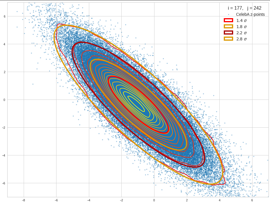
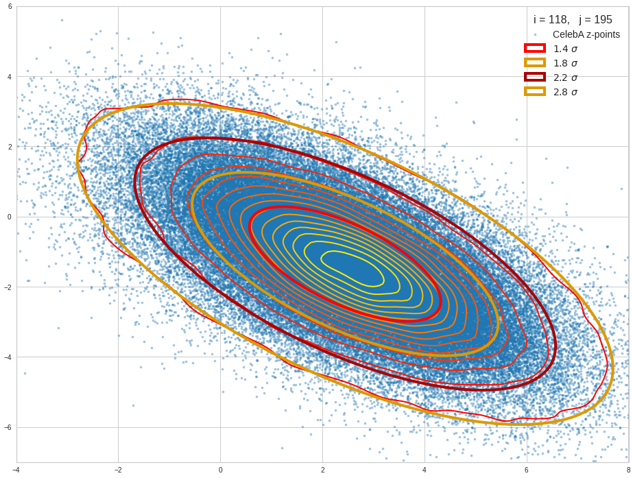
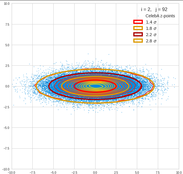
In my present working context ellipses appear as a side result of statistical multivariate normal distributions [MNDs]. The projections of multidimensional contour hyper-surfaces of a MND within the ℝn onto coordinate planes of an Cartesian Coordinate System [CCS] result in 2-dimensional ellipses. These ellipses are typically rotated against the axes of the CCS – and their rotation angles reflect data correlations. The general relations of statistical vector data with projections of multidimensional MNDs are somewhat intricate.
Data produced in numerical experiments, e.g. in a Machine Learning context, most often do not give you the geometrical properties of ellipses, which some theory may have predicted, directly. Instead you may get numerical values of statistical vector distributions which correspond to algebraic coefficients. Examples of such coefficients are e.g. correlation coefficients. These coefficients can often be regarded as elements of a matrix. In case of an underlying MND of your statistical variables these matrices indirectly and approximately describe contour surfaces – namely ellipsoids. Or regarding projections of the data on 2-dim coordinate planes “ellipses”.
Ellipsoids/ellipses can in general be defined by matrices operating on position vectors. In particular: Coefficients of quadratic polynomial expressions used to describe ellipses as conic sections correspond to the coefficients of a matrix operating on position vectors.
So, when I became confronted with multidimensional MNDs and their projections on coordinate planes the following questions became interesting:
- How can one derive the lengths σ1, σ2 of the perpendicular principal axes of an ellipse from data for the coefficients of a matrix which defines the ellipse by a polynomial expression?
- By which formula do the matrix coefficients provide the inclination angle of the ellipse’s primary axes with the x-axis of a chosen coordinate system?
You may have to dig a bit to find correct and reproducible answers in your math books. Regarding the resulting mathematical expressions I have had some bad experiences with ChatGPT. But as a former physicist I take the above questions as a welcome exercise in solving quadratic equations and doing some linear algebra. So, for those of my readers who are a bit interested in elementary math I want to answer the posed questions step by step and indicate how one can derive the respective formulas. The level is moderate – you need some knowledge in trigonometry and/or linear algebra.
Centered ellipses and two related matrices
Below I regard ellipses whose centers coincide with the origin of a chosen CCS. For our present purpose we thus get rid of some boring linear terms in the equations we have to solve. We do not loose much of general validity by this step: Results of an off-center ellipse follow from applying a simple translation operation to the resulting vector data. But I admit: Your (statistical) data must give you some relatively precis information about the center of your ellipse. We assume that this is the case.
Our ellipses can be rotated with respect to a chosen CCS. I.e., their longer principal axes may be inclined by some angle φ towards the x-axis of our CCS.
There are actually two different ways to define a centered ellipse by a matrix:
- Alternative 1: We define the (rotated) ellipse by a matrix AE which results from the (matrix) product of two simpler matrices: AE = Rφ ○ Dσ1, σ2.
Dσ1, σ2 corresponds to a scaling operation applied to position vectors for points located on a centered unit circle. Aφ describes a subsequent rotation. AE summarizes these geometrical operations in a compact form. - Alternative 2: We define the (rotated) ellipse by a matrix Aq which combines the x- and y-elements of position vectors in a polynomial equation with quadratic terms in the components (see below). The matrix defines a so called quadratic form. Geometrically interpreted, a quadratic form describes an ellipse as a special case of a conic section. The coefficients of the polynomial and the matrix must, of course, fulfill some particular properties.
While it is relatively simple to derive the matrix elements from known values for σ1, σ2 and φ it is a bit harder to derive the ellipse’s properties from the elements of either of the two defining matrices. I will cover both matrices in this post.
For many practical purposes the derivation of central elliptic properties from given elements of Aq is more relevant and thus of special interest in the following discussion.
Matrix AE of a centered and rotated ellipse: Scaling of a unit circle followed by a rotation
Our starting point is a unit circle C whose center coincides with our CCS’s origin. The components of vectors vc to points on the circle C fulfill the following conditions:
\pmb{C} \::\: \left\{ \pmb{v}_c \:=\: \begin{pmatrix} x_c \\ y_c \end{pmatrix} \:=\: \begin{pmatrix} \operatorname{cos}(\psi) \\ \operatorname{sin}(\psi) \end{pmatrix}, \quad 0\,\leq\,\psi\, \le 2\pi \right\}
\]
and
x_c^2 \, +\, y_c^2 \,=\; 1 \,.
\]
We define an ellipse E(σ1, σ2) by the application of two linear operations to the vectors of the unit circle:
\pmb{E}_{\sigma_1, \, \sigma_2} \::\: \left\{ \, \pmb{v}_E \:=\: \begin{pmatrix} x_E \\ y_E \end{pmatrix} \:=\: \pmb{\operatorname{R}}_{\phi} \circ \pmb{\operatorname{D}}_E \circ \pmb{v}_c , \quad \pmb{v_c} \in \pmb{C} \, \right\} \,.
\]
DE is a diagonal matrix which describes a stretching of the circle along the CCS-axes, and Rφ is an orthogonal rotation matrix. The stretching (or scaling) of the vector-components is done by
\pmb{\operatorname{D}}_E \:=\: \begin{pmatrix} \sigma_1 & 0 \\ 0 & \sigma_2 \end{pmatrix} \,,
\]
\pmb{\operatorname{D}}_E^{-1} \:=\: \begin{pmatrix} {1 / \sigma_1} & 0 \\ 0 & {1 / \sigma_2} \end{pmatrix} \,.
\]
The coefficients σ1, σ2 obviously define the lengths of the principal axes of the yet unrotated ellipse.
To be more precise: σ2 is half of the diameter in y-direction. I.e. σ1 and σ2 refer to the half-axes of the ellipse.
The subsequent rotation by an angle φ against the x-axis of the CCS is done by
\pmb{\operatorname{R}}_{\phi} \:=\:
\begin{pmatrix} \operatorname{cos}(\phi) & – \,\operatorname{sin}(\phi) \\ \operatorname{sin}(\phi) & \operatorname{cos}(\phi)\end{pmatrix}
\:=\: \begin{pmatrix} u_1 & -\,u_2 \\ u_2 & u_1 \end{pmatrix} \,,
\]
\pmb{\operatorname{R}}_{\phi}^T \:=\: \pmb{\operatorname{R}}_{\phi}^{-1} \:=\: \pmb{\operatorname{R}}_{-\,\phi} \,\,.
\]
The combined linear transformation results in a matrix AE with coefficients ((a, b), (c, d)):
\pmb{\operatorname{A}}_E \:=\: \pmb{\operatorname{R}}_{\phi} \circ \pmb{\operatorname{D}}_E \:=\:
\begin{pmatrix} \sigma_1\,u_1 & -\,\sigma_2\,u_2 \\ \sigma_1\,u_2 & \sigma_2\,u_1 \end{pmatrix} \:=\:: \begin{pmatrix} a & b \\ c & d \end{pmatrix} \,\,.
\end{align}
\]
These is the first set of matrix coefficients we are interested in.
Note:
\begin{pmatrix} {1 \over \sigma_1} \,u_1 & {1 \over \sigma_1}\,u_2 \\ -{1 \over \sigma_2}\,u_2 & {1 \over \sigma_2}\,u_1 \end{pmatrix} \, ,
\]
\pmb{v}_E \:=\: \begin{pmatrix} x_E \\ y_E \end{pmatrix} \:=\: \pmb{\operatorname{A}}_E \circ \begin{pmatrix} x_c \\ y_c \end{pmatrix} \,,
\]
\pmb{v}_c \:=\: \begin{pmatrix} x_c \\ y_c \end{pmatrix} \:=\: \pmb{\operatorname{A}}_E^{-1} \circ \begin{pmatrix} x_E \\ y_E \end{pmatrix} \, .
\]
We use
&u_1 \,=\, \operatorname{cos}(\phi),\quad u_2 \,=\,\operatorname{sin}(\phi), \quad u_1^2 \,+\, u_2^2 \,=\, 1 \,,\\[8pt]
&(1/\lambda_1) \,: =\, \sigma_1^2, \quad\quad (1/\lambda_2) \,: =\, \sigma_2^2
\end{align}
\]
and find
a \,&=\, \sigma_1\,u_1, \quad b \,=\, -\, \sigma_2\,u_2 \,, \\[8pt]
c \,&=\, \sigma_1\,u_2, \quad d \,=\, \sigma_2\,u_1 \,,
\end{align}
\]
\operatorname{det}\left( \pmb{\operatorname{A}}_E \right) \:=\: a\,d \,-\, b\,c \:=\: \sigma_1\, \sigma_2 \,.
\]
As we already know, σ1 and σ2 are factors which give us the lengths of the principal axes of the ellipse. σ1 and σ2 have positive values. We, therefore, can safely assume:
\operatorname{det}\left( \pmb{\operatorname{A}}_E \right) \:=\: a\,d \,-\, b\,c \:\gt\: 0
\]
Ok, we have defined an ellipse via an invertible matrix AE, whose coefficients are directly based on geometrical properties.
But as said: Often an ellipse is described by a an equation with quadratic terms in x and y coordinates of data points. The quadratic form has its background in algebraic properties of conic sections. As a next step we derive such a quadratic equation and relate the coefficients of the quadratic polynomial with the elements of our matrix AE. The result will in turn define another very useful matrix Aq.
Quadratic forms – Case 1: Centered ellipse, principal axes aligned with CCS-axes
We start with a simple case. We take a so called axis-parallel ellipse which results from applying only a scaling matrix DE onto our unit circle C. I.e., in this case, the rotation matrix is assumed to be just the identity matrix. We can omit it from further calculations:
\pmb{\operatorname{R}}_{\phi} \:=\:
\begin{pmatrix} 1 & 0 \\ 0 & 1 \end{pmatrix} \,=\, \pmb{\operatorname{I}}, \quad u_1 \,=\, 1,\: u_2 \,=\, 0, \: \phi = 0 \,.
\]
We need an expression in terms of (xE, yE).
To get quadratic terms of vector components it often helps to invoke a scalar product. The scalar product of a vector with itself gives us the squared norm or length of a vector. In our case the norms of the inversely re-scaled vectors obviously have to fulfill:
\left[\, \pmb{\operatorname{D}}_E^{-1} \circ \begin{pmatrix} x_E \\ y_E \end{pmatrix} \, \right]^T \,\bullet \, \left[\, \pmb{\operatorname{D}}_E^{-1} \circ \begin{pmatrix} x_E \\ y_E \end{pmatrix} \,\right] \:=\: 1 \,\,.
\]
(The bullet represents the scalar product of the vectors.) This directly results in:
{1 \over \sigma_1^2} * x_E^2 \, + \, {1 \over \sigma_2^2} * y_E^2 \:=\: 1 \,.
\]
We eliminate the denominator to get a convenient quadratic form:
\lambda_1 * x_E^2 \,+\, \lambda_2 * y_E^2 \:=1 \,.
\]
If we were given the quadratic form more generally by coefficients α, β and γ
\alpha * x_E^2 \,+\, \beta * x_E \, y_E \,+\, \gamma * y_E^2 \,:=\, 1 \,,
\]
we could directly relate these coefficients with the geometrical properties of our ellipse:
Axis-parallel ellipse:
\alpha \,&=\, 1 / a^2 \,=\, 1 / \sigma_1^2 \,=\, \lambda_1 \,, \\[8pt]
\gamma \,&=\, 1 / d^2 \,=\, 1 / \sigma_2^2 \,=\, \lambda_2 \,, \\[8pt]
\beta \,&=\, b \,=\, c \,=\, 0 \,, \\[8pt]
\phi &= 0 \,.
\end{align}
\]
I.e., we can directly derive σ1, σ2 and φ from the coefficients of the quadratic form. But an axis-parallel ellipse is a very simple ellipse. Things get more difficult for a rotated ellipse.
Quadratic forms – Case 2: General centered and rotated ellipse
We perform the same trick with the vectors vE to get a quadratic polynomial for a rotated ellipse:
\left[ \,\pmb{\operatorname{A}}_E^{-1} \circ \begin{pmatrix} x_E \\ y_E \end{pmatrix} \, \right]^T \, \bullet \,
\left[ \, \pmb{\operatorname{A}}_E^{-1} \circ \begin{pmatrix} x_E \\ y_E \end{pmatrix} \,\right] \:=\: 1 \,\,.
\]
I skip the lengthy, but simple algebraic calculation. We get (with our matrix elements a, b, c, d):
{1 \over \sigma_1^2 \, \sigma_2^2 } \, \left[ \,
\left( c^2 \,+\, d^2 \right) * x_E^2 \,\, – \,\, 2\left( a\,c\, +\, b\,d \right)* x_E \, y_E \,\, + \,\, \left(a^2 \,+\, b^2\right) * y_E^2 \, \right]
\,=\, 1 \, .
\]
The rotation has obviously lead to mixing of components in the polynomial. The coefficient for xE * yE is > 0 for the non-trivial case.
Quadratic form: A matrix equation to define an ellipse
We rewrite our equation again with general coefficients α, β and γ
\alpha * x_E^2 \, + \, \beta * x_E \, y_E \, + \, \gamma * y_E^2 \,=\, 1 \,.
\]
These are coefficients which may come from some theory or from averages of numerical data.
The quadratic polynomial can in turn be reformulated as a matrix operation with a symmetric matrix Aq:
\pmb{v}_E^T \circ \pmb{\operatorname{A}}_q \circ \pmb{v}_E \:=\: 1 \,,
\]
with
\begin{pmatrix} \alpha & \beta / 2 \\ \beta / 2 & \gamma \end{pmatrix} \,\,,
\]
\begin{pmatrix} c^2 \,+\, d^2 & a\,c \, +\, b\,d \\ a\,c \, +\, b\,d & a^2 \,+\, b^2 \end{pmatrix} \, .
\]
This means
\alpha \:&=\: { 1 \over \sigma_1^2 \, \sigma_2^2} \, \left(\, c^2 \,+\, d^2 \,\right) \:=\: \lambda_2 * u_2^2 \, + \, \lambda_1 * u_1^2 \,, \\[8pt]
\gamma \:&=\: { 1 \over \sigma_1^2 \, \sigma_2^2} \, \left(\, a^2 \,+\, b^2 \,\right) \:=\: \lambda_2 * u_1^2 \, + \, \lambda_1 * u_2^2 \,, \\[8pt]
\beta \:&=\: – \, 2\, { 1 \over \sigma_1^2 \, \sigma_2^2} \, \left(\,a \,c \,+\, b \, d \,\right) \:=\: – \, 2 \, \left( \lambda_2 \,-\, \lambda_1 \right)\, u_1 \, u_2 \,.
\end{align}
\]
With
\]
it follows that
\alpha \:&=\: \lambda_2 * \sin^2 \phi \, + \, \lambda_1 * \cos^2 \phi \,, \\[8pt]
\gamma \:&=\: \lambda_2 * \cos^2 \phi \, + \, \lambda_1 * \sin^2 \phi \,, \\[8pt]
\beta \:&=\: – \, 2 \, \left( \lambda_2 \,-\, \lambda_1 \right)\, \cos \phi \, \sin \phi \,.
\end{align}
\]
These terms are intimately related to the geometrical data; expect them to play a major role in further considerations.
With the help of the coefficients of AE we can also show that det(Aq) > 0:
\operatorname{det}\left( \pmb{\operatorname{A}}_q \right) \:=\: \left(\,\alpha \, \gamma \,-\, {1\over 4}\, \beta^2 \, \right) \:=\: { 1 \over \sigma_1^2 \, \sigma_2^2} \, \left(\, b\,c \,-\, a\,d \, \right)^2 \, \gt \, 0 \,.
\]
Thus Aq is an invertible matrix if AE is invertible. For standard conditions (σ1 >0, σ2 > 0) this is the case (see above). Furthermore, Aq is symmetric and thus its own transposed matrix.
Above we have got α, β, γ as some relatively simple functions of a, b, c, d. The inversion is not so trivial and we do not even try it here.
Instead we focus on how we can express σ1, σ2 and φ as functions of either (a, b, c, d) or (α, β, γ).
How to derive σ1, σ2 and φ from the coefficients of AE or Aq in the general case?
Let us assume we have (numerical) data for the coefficients of the quadratic form. Then we may want to calculate values for the length of the principal axes and the rotation angle φ of the corresponding ellipse. There are two ways to derive respective formulas:
- Approach 1: Use trigonometric relations to directly solve the equation system.
- Approach 2: Use an eigenvector decomposition of Aq.
Both ways are fun!
Direct derivation of σ1, σ2 and φ from Aq by using trigonometric relations
Trigonometric relations which we can use are:
\sin (2 \, \phi) \:&=\: 2 \,\cos (\phi)\, \sin(\phi) \,, \\[8pt]
\cos (2 \, \phi) \:&=\: 2 \,\cos^2 (\phi)\, -\, 1 \\[8pt]
\:&=\: 1 \,-\, 2\,\sin^2(\phi) \\[8pt]
\:&=\: \cos^2 (\phi)\, -\, \sin^2 (\phi) \,.
\end{align}
\]
Without loosing much of generality we further assume
\lambda_2 \:\ge \lambda_1 \,.
\]
This affects some aspects of the following derivations and should be kept in mind whilst reading. In the end, our results would only differ by a rotation of π/2, if we had chosen otherwise.
Note, however, that due to our assumption we discuss ellipses whose half-axis σ1 in x-direction is longer than the half-axis σ2 in y-direction!
By combining the above relations for the Aq-coefficients we find
\alpha \, + \, \gamma \,&=\, \lambda_1 \,+\, \lambda_2 \,, \\[8pt]
\gamma \,\, – \, \alpha \,&=\, \left( \, \lambda_2 \,-\, \lambda_1\,\right) \, \cos (2\,\phi) \,, \\[8pt]
\,-\, \beta \:&=\: \left( \, \lambda_2 \,-\, \lambda_1 \, \right)\, \sin (2\,\phi) \,.
\end{align}
\]
By squaring and adding the last two equations we further get
\lambda_2 \,+\, \lambda_1 \,&=\, \alpha \, + \gamma \,, \\[8pt]
\lambda_2 \,-\, \lambda_1 \,&=\, \left[\, \beta^2 \,+\, \left(\,\gamma \,-\,\alpha \,\right)^2\, \right]^{1/2} \,.
\end{align}
\]
Eventually we conclude:
\lambda_1 \,&=\, {1\over 2}\, \left[\, (\,\alpha\,+\,\gamma\,) \,-\, \left[\, \beta^2 \,+\, \left(\,\gamma \,-\,\alpha \,\right)^2\, \right]^{1/2} \, \right] \,, \\[8pt]
\lambda_2 \,&=\, {1\over 2}\, \left[\, (\,\alpha\,+\,\gamma\,) \,+\, \left[\, \beta^2 \,+\, \left(\,\gamma \,-\,\alpha \,\right)^2\, \right]^{1/2} \, \right] \,.
\end{align}
\]
Note that λ1 indeed is smaller than λ2! This reflects our assumption made above about the lengths of the ellipse’s axes.
For λ2 ≥ λ1 the rotation angle is given by
\phi \:=\: \, {1 \over 2} \operatorname{arcsin}\left( {-\, \beta \over \left[ \beta^2 \, +\, \left( \gamma \,-\, \alpha \right)^2 \, \right]^{1/2} } \right) \,.
\]
See a later section below for ambiguities coming from the arcsin-function. A proper analysis and interpretation of this formula for the rotation angle is necessary, when you want to reconstruct ellipses by numerical methods from a given matrix Aq. Some matrices may describe ellipses with their half-axis in y-direction being longer than the half-axis in x-direction. Then λ1 and λ2 would change their role with respect to x,y.
Example:
A typical example for a matrix would be one that appears in the context of a standardized (!) bivariate normal distribution with some correlation imposed onto the statistical variables:
\begin{pmatrix} 1 & -\,\rho \\ -\,\rho & 1 \end{pmatrix} \,\,,
\]
with ρ > 0 being the Pearson correlation coefficient. For this case we get for the half axes of a respective ellipse and the angle :
\sigma_1 \,& =\, \sqrt{\left(\, 1\,+\, \rho\,\right)\, } \,, \\[8pt]
\sigma_2 \,& =\, \sqrt{\left(\, 1\,-\, \rho\,\right)\, } \,, \\[8pt]
\phi \,& =\, \pi / 4 \,. \\[8pt]
\end{align}
\]
Direct derivation of σ1, σ2 and φ from AE by using trigonometric relations
We set
\epsilon_1 \,&=\, \sigma_1^2 \,=\, {1 \over \lambda_1 } \,, \\[8pt]
\epsilon_2 \,&=\, \sigma_2^2 \,=\, {1 \over \lambda_2 } \,.
\end{align}
\]
We have:
a^2 \,+\, b^2 \:&=\: \epsilon_1 * \cos^2 \phi \, + \, \epsilon_2 * \sin^2 \phi \,, \\[8pt]
c^2 \,+\, d^2 \:&=\: \epsilon_1 * \sin^2 \phi \, + \, \epsilon_2 * \cos^2 \phi \,, \\[8pt]
a\, c \,+\, b\, d \:&=\: \left( \, \epsilon_1 \,-\, \epsilon_2 \, \right) * \cos \phi * \sin \phi \,.
\end{align}
\]
This leads to
2 \,\left( \, a^2 \,+\, b^2 \, \right) \:&=\: \epsilon_1 * \left(\, 1 \,+\, \cos (2\phi) \, \right) \, + \, \epsilon_2 * \left( \, 1 \,-\, \cos (2\phi) \, \right) \,, \\[8pt]
2 \,\left( \, c^2 \,+\, d^2 \, \right) \:&=\: \epsilon_2 * \left(\, 1 \,+\, \cos (2\phi) \, \right) \, + \, \epsilon_1 * \left( \, 1 \,-\, \cos (2\phi)\, \right) \,, \\[8pt]
2 \, \left(\,a \,c \,+\, b\, d \,\right) \:&=\: \left(\, \epsilon_1 \,-\, \epsilon_2 \, \right) * \sin (2\phi) \,.
\end{align}
\]
We rearrange terms and get:
\epsilon_1 \,+\, \epsilon_2 \, +\, \left( \epsilon_1 \,-\, \epsilon_2 \right) * \cos (2\phi) \:&=\: \,+ 2 \, \left( \, a^2 \,+\, b^2 \, \right) \,, \\[8pt]
\,-\, \epsilon_1 \,-\, \epsilon_2 \,+\, \left( \epsilon_1 \,-\, \epsilon_2 \right) * \cos (2\phi) \:&=\: \,- 2 \, \left( \, c^2 \,+\, d^2 \, \right) \,, \\[8pt]
\left(\, \epsilon_1 \,-\, \epsilon_2 \, \right) * \sin (2\phi) \:&=\: \,+ 2 \, \left( \, a\,c \,+\, b\,d \, \right) \,.
\end{align}
\]
Let us define some further variables before we add and subtract the first two of the above equations:
r \:&=\: {1 \over 2} \left(\, a^2 \,+\, b^2 \,+\, c^2 \,+\, d^2 \, \right) \,, \\[8pt]
s_1 \:&=\: {1 \over 2} \left(\, a^2 \,+\, b^2 \,-\, c^2 \,-\, d^2 \, \right) \,, \\[8pt]
s_2 \:&=\: \left(\, a\,c \,+\, b\,d \, \right) \,, \\[8pt]
\pmb{s} \:&=\: \begin{pmatrix} s_1 \\ s_2 \end{pmatrix} \,, \\[8pt]
s \:&=\: \sqrt{ s_1^2 \,+\, s_2^2 } \, .
\end{align}
\]
Adding two of the equations with the sin(2φ) and cos(2φ) above and using the third equation results in:
{1 \over 2} \, \left( \epsilon_1 \,-\, \epsilon_2 \right) \begin{pmatrix} \cos (2\phi) \\ \sin (2\phi) \end{pmatrix} \:=\: \begin{pmatrix} s_1 \\ s_2 \end{pmatrix} \,.
\]
Taking the vector norm on both sides (with ε1 ≥ ε2) and adding two of the equations above results in:
\epsilon_1 \,\, – \,\, \epsilon_2 \:&=\: 2 * s \,, \\[8pt]
\epsilon_1 \, + \, \epsilon_2 \:&=\: 2 * r \,.
\end{align}
\]
This gives us:
\sigma_1^2 \,=\, \epsilon_1 \:&=\: r \,+\, s \,, \\[8pt]
\sigma_2^2 \,=\, \epsilon_2 \:&=\: r \,-\, s \,.
\end{align}
\]
In terms of the coefficients a, b, c, d:
\sigma_1^2 \,=\, {1 \over \lambda_1} \:&=\: {1 \over 2} \left[ \, a^2+b^2+c^2 +d^2 \,+\, \left[ 4 (ac + bd)^2 \, +\, \left( c^2+d^2 -a^2 -b^2\right)^2 \, \right]^{1/2} \right] \,, \\[8pt]
\sigma_2^2 \,=\, {1 \over \lambda_2} \:&=\: {1 \over 2} \left[ \, a^2+b^2+c^2 +d^2 \,-\, \left[ 4 (ac + bd)^2 \, +\, \left( c^2+d^2 -a^2 -b^2\right)^2 \, \right]^{1/2} \right] \,.
\end{align}
\]
Who said that life had to be easy?
But, it is relatively easy to prove:
\sigma_1^2 * \sigma_2^2 \,=\, {1 \over \lambda_1^2 \, \lambda_2^2} \,=\, \left(\, a\,d\,-\, b\,c\ \, \right)^2 \,=\, \left[\operatorname{det}\left(\pmb{\operatorname{A}}_q \right)\right]^2 \,.
\]
So, we can indeed confirm :
\alpha \:&=\: { 1 \over \left(\,a\,d \,-\, b\,c\,\right)^2 } \, \left(\, c^2 \,+\, d^2 \,\right) \,, \\[8pt]
\gamma \:&=\: { 1 \over \left(\,a\,d \,-\, b\,c\,\right)^2 } \, \left(\, a^2 \,+\, b^2 \,\right) \,, \\[8pt]
\beta \:&=\: – \, 2\, { 1 \over \left(\,a\,d \,-\, b\,c\,\right)^2 } \, \left(\,a \,c \,+\, b \, d \,\right)\,.
\end{align}
\]
Determination of the inclination angle φ
For the determination of the angle φ we use:
\begin{pmatrix} \operatorname{cos}(2\phi) \\ \operatorname{sin}(2\phi) \end{pmatrix} \:=\: {1 \over s} \begin{pmatrix} s_1 \\ s_2 \end{pmatrix} \,.
\]
We choose
-\pi/2 \,\lt\, \phi \le \pi/2 \,,
\]
and get:
\phi \:=\: {1 \over 2} \operatorname{arctan}\left({s_2 \over s_1}\right) \:=\: {1 \over 2} \, \operatorname{arctan}\left( { 2\left(ac \,+\, bd\right) \over (a^2 \,+\, b^2 \,-\, c^2 \,-\, d^2) } \right) \,.
\]
Note: All in all there are four different solutions. The reason is that we alternatively could have requested λ2 ≥ λ1 and also chosen the angle π + φ. So, the ambiguity is due to a selection of the considered principal axis and rotational symmetries.
2nd way to a solution for σ1, σ2 and φ via eigendecomposition
For our second way of deriving formulas for σ1, σ2 and φ we use some linear algebra.
This approach is interesting for two reasons: It indicates how we can use the Python “linalg”-package together with Numpy to get results numerically. In addition we get familiar with a representation of the ellipse in a properly rotated CCS.
Above we have written down a symmetric matrix Aq describing an operation on the position vectors of points on our rotated ellipse:
\pmb{v}_E^T \circ \pmb{\operatorname{A}}_q \circ \pmb{v}_E \:=\: 1 \,.
\]
We know from linear algebra that every symmetric matrix can be decomposed into a product of orthogonal matrices O, OT and a diagonal matrix. This reflects the so called eigendecomposition of a symmetric matrix. It is a unique decomposition in the sense that it has a uniquely defined solution in terms of the coefficients of the following matrices:
\pmb{\operatorname{A}}_q \:=\: \pmb{\operatorname{O}} \circ \pmb{\operatorname{D}}_{diag} \circ \pmb{\operatorname{O}}^T
\]
with
\pmb{\operatorname{D}}_{diag} \:=\: \begin{pmatrix} \lambda_{u} & 0 \\ 0 & \lambda_{d} \end{pmatrix}
\]
The coefficients λu and λd are eigenvalues of both Ddiag and Aq.
Reason:
Orthogonal matrices do not change eigenvalues of a transformed matrix. So, the diagonal elements of Ddiag are the eigenvalues of Aq. Linear algebra also tells us that the columns of the matrix O are given by the components of the normalized eigenvectors of Aq.
We can interpret O as a rotation matrix Rψ for some angle ψ:
\pmb{v}_E^T \circ \pmb{\operatorname{A}}_q \circ \pmb{v}_E \:=\: \pmb{v}_E^T \circ
\pmb{\operatorname{R}}_{\psi} \circ \pmb{\operatorname{D}}_{diag} \circ \pmb{\operatorname{R}}_{\psi}^T \circ \pmb{v}_E \:=\: 1 \,.
\]
This means
\left[ \pmb{\operatorname{R}}_{-\psi} \circ \pmb{v}_E \right]^T \circ
\pmb{\operatorname{D}}_{diag} \circ \left[ \pmb{\operatorname{R}}_{-\psi} \circ \pmb{v}_E \right] \:=\: 1 \,.
\]
The whole operation tells us a simple truth, which we are already familiar with. By our construction procedure for a rotated ellipse we know that a rotated CCS exists, in which the ellipse can be described as the result of a scaling operation (along the coordinate axes of the rotated CCS) applied to a unit circle. (This CCS is, of course, rotated by an angle φ against our working CCS in which the ellipse appears rotated.)
Above we had found
\left[ \,\pmb{\operatorname{A}}_E^{-1} \circ \begin{pmatrix} x_E \\ y_E \end{pmatrix} \, \right]^T \, \bullet \,
\left[ \, \pmb{\operatorname{A}}_E^{-1} \circ \begin{pmatrix} x_E \\ y_E \end{pmatrix} \,\right] \:=\: 1
\]
With our matrices Rφ and scaling matrix DE we can rewrite this as
\left[ \begin{pmatrix} x_E \\ y_E \end{pmatrix} \, \right]^T \, \circ \,
\left[ \pmb{\operatorname{D}}_E^{-1} \circ \pmb{\operatorname{R}}_{-\phi} \right]^T \bullet
\left[ \pmb{\operatorname{D}}_E^{-1} \circ \pmb{\operatorname{R}}_{-\phi} \right] \circ \begin{pmatrix} x_E \\ y_E \end{pmatrix} \:=\: 1 \,.
\]
So:
\left[ \begin{pmatrix} x_E \\ y_E \end{pmatrix} \, \right]^T \, \circ \,
\left[ \pmb{\operatorname{R}}_{-\phi} \right]^T \circ \left[ \pmb{\operatorname{D}}_E^{-1} \right]^T \circ
\pmb{\operatorname{D}}_E^{-1} \circ \pmb{\operatorname{R}}_{-\phi} \circ \begin{pmatrix} x_E \\ y_E \end{pmatrix} \:=\: 1 \,.
\]
Remembering that a diagonal matrix is its own transposed matrix and that the inverse of an orthogonal matrix (rotation) is its transposed matrix, we get:
\left[ \begin{pmatrix} x_E \\ y_E \end{pmatrix} \, \right]^T \, \circ \,
\left[ \pmb{\operatorname{R}}_{\phi} \right] \circ \left[ \pmb{\operatorname{D}}_E^{-1} \circ
\pmb{\operatorname{D}}_E^{-1} \right] \circ \pmb{\operatorname{R}}_{\phi}^T \circ \begin{pmatrix} x_E \\ y_E \end{pmatrix} \:=\: 1 \,.
\]
Comparing expressions, we find
\pmb{\operatorname{D}}_{diag} \:=\: \left[ \pmb{\operatorname{D}}_E^{-1} \circ
\pmb{\operatorname{D}}_E^{-1} \right] \,.
\]
And thus, following our old assumption λ1 ≤ λ2 (!) – we set
\lambda_u \,=\, \lambda_1 \,&=\, {1 \over \sigma_1^2} \,, \\[8pt]
\lambda_d \,=\, \lambda_2 \,&=\, {1 \over \sigma_2^2} \,.
\end{align} \]
The eigenvalues of our symmetric matrix Aq are just our parameters λ1 and λ2.
It is really noteworthy that the half-axes of the ellipse are given by the reciprocate value of the square root of the matrix’ eigenvalues:
\sigma_1 \:&=\: {1 \over \sqrt{\lambda_1} } \,, \\[8pt]
\sigma_2 \:&=\: {1 \over \sqrt{\lambda_2} } \,.
\end{align} \]
Mathematically, a lengthy calculation (see below) will indeed reveal that the eigenvalues of a symmetric matrix Aq with coefficients α, 1/2*β and γ have the following form:
\lambda_{1/2} \:=\: \lambda_{u/d} \:=\: {1 \over 2} \left[\, \left(\alpha \,+\, \gamma \right) \,\mp\, \left[ \beta^2 + \left(\gamma \,-\, \alpha \right)^2 \,\right]^{1/2} \, \right]
\]
Side remark: You can derive this results a bit easier with solving the so called “characteristic equation” of the matrix. For more details see e.g.:
Eigenvalues and eigenvector of a positive-definite, real valued and symmetric matrix
This is, of course, exactly what we have found some minutes ago by solving respective equations with the help of trigonometric terms. Remember, however, the assumptions about the λ-values and lengths of the ellipse’s axes!
We will prove the fact that these indeed are valid eigenvalues in a minute. Let us first look at respective eigenvectors ξ1/2. To get them we must solve the equations resulting from
\left( \begin{pmatrix} \alpha & \beta / 2 \\ \beta / 2 & \gamma \end{pmatrix} \,-\, \begin{pmatrix} \lambda_{1/2} & 0 \\ 0 & \lambda_{1/2} \end{pmatrix} \right) \,\circ \, \pmb{\xi_{1/2}} \:=\: \pmb{0},
\]
with
\pmb{\xi_1} \,=\, \begin{pmatrix} \xi_{1,x} \\ \xi_{1,y} \end{pmatrix}, \quad \pmb{\xi_2} \,=\, \begin{pmatrix} \xi_{2,x} \\ \xi_{2,y} \end{pmatrix}
\]
Below we will show that the following vectors fulfill the conditions (up to a common factor in the components):
\lambda_1 \: &: \quad \pmb{\xi_1} \:=\: \left(\, {1 \over \beta} \left( (\alpha \,-\, \gamma) \,-\, \left[\, \beta^2 \,+\, \left(\gamma \,-\, \alpha \right)^2\,\right]^{1/2} \right), \: 1 \, \right)^T \,, \\[8pt]
\lambda_2 \: &: \quad \pmb{\xi_2} \:=\: \left(\, {1 \over \beta} \left( (\alpha \,-\, \gamma) \,+\, \left[\, \beta^2 \,+\, \left(\gamma \,-\, \alpha \right)^2\,\right]^{1/2} \right), \: 1 \, \right)^T \,.
\end{align}
\]
for the eigenvalues
\lambda_1 \:&=\: {1 \over 2} \left(\, \left(\alpha \,+\, \gamma \right) \,-\, \left[ \beta^2 \,+\, \left(\gamma \,-\, \alpha \right)^2 \,\right]^{1/2} \, \right) \,, \\[8pt]
\lambda_2 \:&=\: {1 \over 2} \left(\, \left(\alpha \,+\, \gamma \right) \,+\, \left[ \beta^2 \,+\, \left(\gamma \,-\, \alpha \right)^2 \,\right]^{1/2} \, \right) \,.
\end{align}
\]
As usual, the T at the formulas for the vectors symbolizes a transposition operation.
Note again that we have
\lambda_1 \:\le\: \lambda_2 \,.
\]
This reflects our initial assumptions about the axes-lenghts of our ellipses. It means that the eigenvalue λ1 and the respective eigenvector ξ1 are associated with the longer half-axis of the ellipse! We had assumed that this half-axis is aligned with the x-coordinate axis.
Note also that the vector components given above are not normalized. This is important for performing numerical checks as Numpy and linear algebra programs would typically give you normalized eigenvectors with a length = 1. But you can easily compensate for this by working with
\lambda_1 \: &: \quad \pmb{\xi_1^n} \:=\: {1 \over \|\pmb{\xi_1}\|}\, \pmb{\xi_1} \,, \\[8pt]
\lambda_2 \: &: \quad \pmb{\xi_2^n} \:=\: {1 \over \|\pmb{\xi_2}\|}\, \pmb{\xi_2} \,.
\end{align}
\]
Proof for the eigenvalues and eigenvector components
We just prove that the eigenvector conditions are e.g. fulfilled for the components of the first eigenvector ξ1 and λ1 = λu.
\left(\alpha \,-\, \lambda_1 \right) * \xi_{1,x} \,+\, {1 \over 2} \beta * \xi_{1,y} \,&=\, 0 \\[8pt]
{1 \over 2} \beta * \xi_{1,x} \,+\, \left( \gamma \,-\, \lambda_1 \right) * \xi_{2,y} \,&=\, 0
\end{align}
\]
(The steps for the second eigenvector are completely analogous).
We start with the condition for the first component:
&\left( \alpha \,-\,
{1\over 2}\left[\,\left(\alpha \, + \, \gamma\right) \,-\, \left[ \beta^2 \,+\, \left( \alpha \,-\, \gamma \right)^2 \right]^{1/2} \right] \right) * \\[8pt]
& {1 \over \beta}\,
\left[\, \left(\alpha \,-\, \gamma\right) \,-\, \left[ \beta^2 \,+\, \left(\alpha \,-\, \gamma \right)^2 \right]^{1/2} \,\right] \,+\, {\beta \over 2 }
\,=\, 0
\end{align}
\]
& {1 \over 2 } \left[ \left(\alpha \,-\,\gamma\right) \,+\, \left[ \beta^2 \,+\, \left( \alpha \,-\, \gamma \right)^2 \right]^{1/2} \right] * \\[8pt]
& {1 \over \beta}\,
\left[\, \left(\alpha \,-\, \gamma\right) \,-\, \left[ \beta^2 \,+\, \left(\alpha \,-\, \gamma \right)^2 \right]^{1/2} \,\right] \,+\, {\beta \over 2 }
\,=\, 0 \,.
\end{align}
\]
{1 \over 2 \, \beta} \left[ (\alpha \,-\,\gamma)^2 \,-\, \beta^2 \,-\, (\alpha \,-\,\gamma)^2 \right] \,+\, {\beta \over 2 } \,=\, 0
\]
The last relation is obviously true.
You can perform a similar calculation for the other eigenvector component:
{1 \over 2} \, \beta & {1 \over \beta}\,
\left[\, \left(\alpha \,-\, \gamma\right) \,-\, \left[ \beta^2 \,+\, \left(\alpha \,-\, \gamma \right)^2 \right]^{1/2} \,\right] \,+\, \\
&
\left( \gamma \, -\,
{1\over 2}\left[\,\left(\alpha \, + \, \gamma\right) \,-\, \left[ \beta^2 \,+\, \left( \alpha \,-\, \gamma \right)^2 \right]^{1/2} \right] \right) * 1 \,=\, 0
\end{align}
\]
Thus:
&{1 \over 2} \, \left(\alpha \,-\, \gamma\right) \,-\, {1 \over 2} \left[ \beta^2 \,+\, \left(\alpha \,-\, \gamma \right)^2 \right]^{1/2} \\
-\, &{1\over 2}\left(\alpha \,-\, \gamma\right) \,+\, {1\over 2}\left[ \beta^2 \,+\, \left( \alpha \,-\, \gamma \right)^2 \right]^{1/2} \,=\, 0
\end{align}
\]
True, again.
In a very similar exercise one can show that the scalar product of the eigenvectors is equal to zero:
& {1 \over \beta^2}\,
\left[\, \left(\alpha \,-\, \gamma\right)^2 \,-\, \beta^2 \,+\, \left(\alpha \,-\, \gamma \right)^2 /\,\right] \,+\, 1 \\[8pt]
& – {1 \over \beta^2} * \beta^2 \,*\,1 \,=\, 0 \,.
\end{align}
\]
I.e.,
\pmb{\xi_1} \bullet \pmb{\xi_1} \,=\, \left( \xi_{1,x}, \, \xi_{1,y} \right) \circ \begin{pmatrix} \xi_{2,x} \\ \xi_{2,y} \end{pmatrix} \,= \, 0 \,.
\]
The eigenvectors are perpendicular to each other. Exactly, what we expect for the orientations of the principal axes of an ellipse against each other.
Rotation angle from coefficients of Aq
We still need a formula for the rotation angle(s). From linear algebra results related to an eigendecomposition we know that the orthogonal (rotation) matrices consist of columns of the normalized eigenvectors. With the components given in terms of our un-rotated CCS, in which we basically work. These vectors point along the principal axes of our ellipse. Thus the components of these eigenvectors define our aspired rotation angles of the ellipse’s principal axes against the x-axis of our CCS.
Let us prove this. By assuming
\cos (\phi_1) \,&=\, \xi_{1,x}^n \,, \\[8pt]
\sin (\phi_1) \,&=\, \xi_{1,y}^n
\end{align}
\]
and using
\sin(2\phi_1) \,=\, 2\, \sin (\phi_1) \, \cos (\phi_1) \,,
\]
we get
\sin (2 \phi_1) \,=\,
2 * { \xi_{1,x} * \xi_{1,y} \over \left[\, \xi_{1,x}^2 \, + \, \xi_{1,y}^2 \,\right] } \,.
\end{align}
\]
Thus
\operatorname{sin}(2 \phi_1) \,&=\,
2 \,\, { {1 \over \large{\beta}} \left( (\alpha \,-\, \gamma) \,-\, \left[\, \beta^2 \,+\, \left(\gamma \,-\, \alpha \right)^2\,\right]^{1/2} \right) \,*\, 1
\over
\left[\, \left( {1 \over \large{\beta}} \left( (\alpha \,-\, \gamma) \,-\, \left[\, \beta^2 \,+\, \left(\gamma \,-\, \alpha \right)^2\,\right]^{1/2} \right) \right)^2
\,+\, 1^2 \right] } \\[8pt]
&=\, 2\,\, { {1 \over \large{\beta}} \left( t \,-\, z \right)
\over
{1 \over \large{\beta}^2 \phantom{\large{]}} } \left[\, \beta^2 \,+\, \left(\, t \,-\, z \,\right)^2 \right] } \,,
\end{align}
\]
with
t \,&=\, (\alpha \,-\, \gamma) \,, \\[8pt]
z \,&=\, \left[\, \beta^2 \,+\, \left(\gamma \,-\, \alpha \right)^2\,\right]^{1/2} \,.
\end{align}
\]
This looks very differently from the simple expression we got above. And a direct approach is cumbersome. The trick is to multiply nominator and denominator by a convenience factor
\left( t \,+\, z \right),
\]
and exploit
\left( t \,-\, z \right) \, \left( t \,+\, z \right) \,&=\, t^2 \,-\, z^2 \,, \\[8pt]
\left( t \,-\, z \right) \, \left( t \,+\, z \right) \,&=\,\, – \,\beta^2
\end{align}
\]
to get
&2 * \beta \, { (t\,-\, z) * ( t\,+\, z) \over \left[ \beta^2 \, + \,( t \,-\, z )^2 \right] * (t \,+\, z) } \\[8pt]
&=\: 2 * \beta \, { – \beta^2 \over \beta^2 (t\,+\,z) \,-\, \beta^2 (t\,-\,z) } \\
&=\: – \, {\beta \over \left[\, \beta^2 \,+\, (\alpha \,-\, \gamma)^2 \,\right]^{1/2} } \,.
\end{align}
\]
This means that our 2nd approach gives us the result
\operatorname{sin}\, (2 \phi_1) \:=\: \, – \, { \beta \over \left[\, \beta^2 \,+\, (\alpha \,-\, \gamma)^2 \,\right]^{1/2} }\,,
\]
which is of course identical to the result we got with our first solution approach. It is clear that the second axis has an inclination by φ +- π / 2:
\phi_2\, =\, \phi_1 \,\pm\, \pi/2.
\]
In general the angles have a natural ambiguity of π. This makes life a bit harder when you get a matrix, use the formulas above and try to construct the matrix with correct orientation.
Addendum 07/05/2025: Getting the right orientation of the ellipses when constructing them via eigenvalues of a matrix Aq
The formulas for the rotation angle of the ellipse look simple. However, some pitfalls may await you, when you want to use the formula to construct your ellipses after having determined its half-axes from the eignevalues of a given matrix Aq. If you are not careful and forget to take into account our special assumptions on axis-length and orientation of the eigenvectors you may get the ellipses orientation wrong.
Most often this happens when working with contour ellipses of BivariateNormal Distributions [BVDs] and their central covariance matrices, which correspond to our Aq-matrix. In the case of BVDs the matrix coefficients have an association with the standard-deviations of the BVDs marginal distributions and this may lead to confusion.
The important points to take care of are the following:
- The arcsin-function allows for multiple equivalent values – and we have to choose the right one. To do this you should analyze both of the key equations determining the angle Φ:
\[ \begin{align}
\gamma \,\, – \, \alpha \,&=\, \left( \, \lambda_2 \,-\, \lambda_1\,\right) \, \cos (2\,\phi) \,, \\[8pt]
\,-\, \beta \:&=\: \left( \, \lambda_2 \,-\, \lambda_1 \, \right)\, \sin (2\,\phi) \,.
\end{align}
\]This will narrow down the interval in which Φ resides.
- Throughout our text, we have used the assumption λ1 = λu ≤ λ2 = λd. A priori it is questionable whether this covers all necessary cases during the reconstruction of an ellipse properly.
Not all given matrices may fulfill the assumption about the λ-values. Instead, for certain matrices the eigenvalues λ1 and λ2 may switch their position in the central diagonal matrix of the eigendecomposition. This must be analyzed.
It can, however, be shown that cases with λ1 < λ2 can be mapped 1:1 onto certain cases with λ1 > λ2. A proper analysis is given in an extensive post in another blog. - The eigenvalue λ1 and the respective eigenvector ξ1 were in our considerations always associated with the longer half-axis of the ellipse! This has the consequence that the meaning of Φ1 during reonstruction can change with respect to the real situation given by the matrix.
A thorough analysis of how the matrix elements determine the angle of the ellipse and respective recipes has meanwhile benn provided by myself in a related post in another blog. There you find also arguments why it is justified to focus on cases with (λ2 – λ1) ≥ 0.
Conclusion
In this post I have shown how one can derive essential properties of centered, but rotated ellipses from matrix-based representations. Such calculations become relevant when e.g. experimental or numerical data only deliver the coefficients of a quadratic form for the ellipse.
We have first established the relation of the coefficients of a matrix that defines an ellipse by a combined scaling and rotation operation with the coefficients of a matrix which defines an ellipse as a quadratic form of the components of position vectors. In addition we have shown how the coefficients of both matrices are related to quantities like the lengths of the principal axes of the ellipse and the inclination of these axes against the x-axis of the Cartesian coordinate system in which the ellipse is described via position vectors. So, if one of our two defining matrices is given we can numerically calculate the ellipse’s main properties.
Regarding the ellipses orientation we have to be careful and check which of its eigenvalues describes the longer axis.
In the next post of this mini-series
Properties of ellipses by matrix coefficients – II – coordinates of points with extremal y-values
we have a look at the x- and y-coordinates of points on an ellipse with extremal y-values. All in terms of the matrix coefficients we are now familiar with.