
This post requires Javascript to display formulas!
In the previous posts of this series we got acquainted with shear operations:
Fun with shear operations and SVD – I – shear matrices and examples created with Blender
Fun with shear operations and SVD – II – Shearing of rectangles and cubes with Python and Matplotlib
Fun with shear operations and SVD – III – Shearing of circles
Already established results for shearing a circle
Post III focused on the shearing of a circle, which was centered in the Euclidean coordinate system [ECS] we worked with. The shear operation resulted in an ellipse with an inclination against the coordinate axes of our ECS. This was interesting regarding four points:
- A circle, which is centered in a chosen ECS, exhibits a continuous rotational symmetry (isotropy). This obviously allows for a decomposition of a shear operation into a sequence of two affine operations in the chosen ECS: a scaling operation (with different factors along the coordinate axes) followed by a rotation (or the other way round). Equivalently: We could switch to another specific ECS which is already rotated by a proper angle against our originally chosen ECS and just perform a scaling operation there.
The rotation angle is determined by the shear parameter λ.
This seems to stand in some contrast to the shearing of figures with only discrete rotational symmetries: We saw for rectangles and cubes that an additional rotation was required to replace the shear operation by a sequence of scaling and rotation operations. - Points (x, y) of circles and ellipses are described by quadratic forms in two dimensions (with some real coefficients α, β, γ, δ):
\[
\alpha \,x^2 \, + \, \beta \, x \, y \, + \, \gamma \, y^2 \:=\: \delta
\]Quadratic forms play a general role in the mathematical description of cone-sections. (Ellipses are the results of specific cone-sections.)
- Ellipses also result from projections of multi-dimensional ellipsoids onto two-dimensional coordinate planes. Multi-dimensional ellipsoids are described by quadratic forms in an ECS covering the ℝn.
- Hyper-surfaces for constant probability density values of multivariate normal vector distributions form multi-dimensional ellipsoids. Here we have a link to Machine Learning where key properties of certain objects are often ruled by Gaussian distributions.
From the first point we may expect that a shear operation applied to a multi-dimensional sphere will result in a multi-dimensional ellipsoid – and that such an operation could be replaced by scaling the original sphere (with different factors along n coordinate axes of a n-dimensional ECS) followed by a rotation (or vice versa). We will explicitly investigate this for a 3-dimensional sphere in the next post.
If our assumption were true we would get a first glimpse of the fact that a general multivariate standard distribution can be created by applying a sequence of distinct affine (i.e. linear) operations to a spherical probability distribution. This is discussed in detail in another post-series in this blog.
What is a bit confusing at the moment is that a replacement of a shear operation by simpler affine operations in general seems to require at least two rotations, but only one when we work with centered isotropic bodies. We come back to this point when we discuss the decomposition of a shear matrix by the so called SVD-procedure.
In the previous post of this series we have used the radius of the circle and the shearing parameter λ to derive analytical expressions for the coordinates of special points with extremal values on our ellipse
- Points with maximal and minimal y-coordinate values.
- Points with a maximal or minimal distance to the symmetry center of the ellipse. I.e. the end-points of the principal diameters of the ellipse.
From the fact that shearing does not change extremal values along the axis perpendicular to the sharing direction we could easily determine the lengths of the ellipse’s principal axes and the inclination angle of the longer axis with the x-axis of our Euclidean coordinate system [ECS].
What do we have in addition? In another mini-series on ellipses
Properties of ellipses by matrix coefficients – I – Two defining matrices (and two more posts)
I have meanwhile described how the geometry of an ellipse is related to its quadratic form and respective coefficients of a symmetric matrix. I call this matrix Aq. It forces the components of position vectors to fulfill an equation based on a quadratic polynomial. Furthermore Aq‘s eigenvalues and eigenvectors define the lengths of the ellipse’s principal axes and their inclination to the axes of our chosen ECS. The matrix coefficients in addition allow us to determine the coordinates of the points with extremal y-values on an ellipse. We will use these results later in the present post.
Objectives of this post: Shearing of a centered, rotated ellipse
In this post I want to show that shearing a given centered, but rotated original ellipse EO results in another ellipse ES with a different inclination angle and different sizes of the principal axes.
In addition we will derive the relations of the shearing parameter λS with the coefficients of the symmetric matrix \(\pmb{\operatorname{A}}_q^S \) that defines ES. I also provide formulas for the dependence of ES‘s geometrical properties on the shear parameter λS.
There are two basic prerequisites:
- We must show that the application of a shear transformation to the variables of the quadratic form which describes an ellipse EO results in another proper quadratic form and a related matrix \(\pmb{\operatorname{A}}_q^S \).
- The coefficients of the resulting quadratic form and of \(\pmb{\operatorname{A}}_q^S \) must fulfill a mathematical criterion for an ellipse.
We expect point 1 to be valid because a shear operation is just a linear operation.
To get some exercise we approach our goals by first looking at the simple case of shearing an axis-parallel ellipse before extending our considerations to general ellipses with an inclination angle against the coordinate axes of our chosen ECS.
Step 1: Shearing of an axis-parallel ellipse
By an “axis-parallel” ellipse I mean an ellipse whose principal axes are aligned with the axes of the 2-dimensional ECS we work in. We can construct such an ellipse Ea by applying a scaling operation to a unit circle. The unit circle may be described by a set of specific position vectors
\pmb{C} \::\: \left\{ \pmb{v}_c \:=\: \begin{pmatrix} x_c \\ y_c \end{pmatrix} \:=\: \begin{pmatrix} \operatorname{cos}(\psi) \\ \operatorname{sin}(\psi) \end{pmatrix}, \quad 0\,\leq\,\psi\, \le 2\pi \right\}
\]
with
x_c^2 \, +\, y_c^2 \,=\; 1
\]
We get an axis-parallel ellipse Ea by applying a scaling matrix
\pmb{E_a} \::\: \left\{ \, \pmb{v}_a \:=\: \begin{pmatrix} x_a \\ y_a \end{pmatrix} \:=\: \pmb{\operatorname{D}} \circ \pmb{v_c} , \quad \pmb{v_c} \in \pmb{C} \, \right\}
\]
D is a diagonal matrix which describes a stretching of the circle along the ECS-axes
\pmb{\operatorname{D}} \:=\: \begin{pmatrix} a_a & 0 \\ 0 & b_a \end{pmatrix},
\]
The matrix coefficients aa and ba obviously define the lengths of the principal axes of our axis-parallel ellipse Ea in x– and y-direction. Let us look at an example
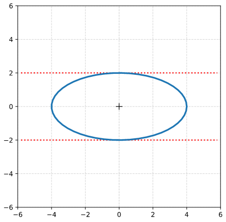
In the depicted case we scaled a unit circle by a factor 2 in y-direction and by a factor 4 in x-direction. I.e.: aa = 4.0 and ba = 2.0.
Mathematically Ea is also defined by a quadratic equation for points (xa, ya) on the ellipse. The position vectors for these points fulfill
b_a^2 \, x_a^2 \,+ \, a_a^2 \, y_a^2 \:=\: a_a^2 \, b_a^2
\]
We apply a shear-operation, i.e. a unipotent matrix with a filled upper triangular part (see post I of this series)
\pmb{\operatorname{M}}_{sh} \: = \: \begin{pmatrix} 1 & \lambda_S \\ 0 & 1 \end{pmatrix}
\]
with a shear-factor λS to the position vectors to get a set ES of sheared vectors
\pmb{E_S} = \left\{\, \pmb{v_S} = \begin{pmatrix} x_S \\ y_S \end{pmatrix}, \right\} \quad \operatorname{with}
\]
\pmb{v_a} \,=\, \begin{pmatrix} x_a \\ y_a \end{pmatrix} \quad \rightarrow \quad \pmb{v_S} \,=\, \begin{pmatrix} x_S \\ y_S \end{pmatrix}
\]
\pmb{v_S} \:=\: \pmb{\operatorname{M}}_{sh} \circ \pmb{v_a}.
\]
I.e.:
\begin{align}
x_S \: &= \: x_a \, + \, \lambda_S * y_a \\
y_S \: &= \: y_a.
\end{align}
\]
We use the quadratic equation for Ea, replace xa, ya by xS and yS and reorder the resulting terms to get
b_a^2 \, x_S^2 \,-\, 2\,b_a^2 \,\lambda_S\,x_S\,y_S \,+\, a_a^2 \, y_S^2 \:=\: a_a^2 \, b_a^2
\]
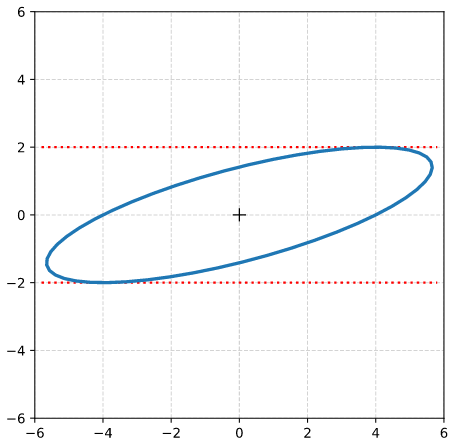
This obviously is a quadratic form again – but with partially different coefficients. The new coefficients actually fulfill the requirement for an ellipse. We will prove this for the general case in the section on step 2, below. So, shearing an axis-parallel ellipse results in a new ellipse with a different geometry.
For our example case we set λS = 2.0 and get:
Next we calculate the components of position vectors to extremal points on ES.
Location of the points with maximum absolute y-values on a sheared, originally axis-parallel ellipse
We know already that
y_S^{ymax} \, = \, y_a \,=\, b_a
\]
We directly get
x_S^{ymax} \, = \, \pm \, \lambda_S \, b_a
\]
Another solution approach is based on a derivative of yS with respect to xS. We define
\eta_a \:=\: {a_a \over b_a}
\]
and reorder terms to get an expression for yS:
y_S \:=\: {1 \over \eta_a^2 \,+\, \lambda_S^2 } \, \left(\, \lambda_S \, x_S \,\pm\, \left[\, a_a^2 \left(\, \eta_a^2 \,+\, \lambda_S^2 \,\right) \,-\, \eta_a^2 \, x_S^2 \,\right]^2 \,\right)
\]
We differentiate and set the derivative to zero:
\begin{align}
{\partial\, y_S \over \partial \, x_S } \:&=\: 0 \\
\Rightarrow \quad \lambda_S \:&=\: \pm\, { -\, \eta_a^2 \, x_S \over \left[\, a_a^2 \left(\, \eta_a^2 \,+\, \lambda_S^2 \,\right) \,-\, \eta_a^2 \, x_S^2 \,\right]^{1/2} }
\end{align}
\]
Getting rid of the denominator and working with a quadratic supplement eventually results in:
\lambda_S^2 \, \left[\, a_a^2 \left(\, \eta_a^2 \,+\, \lambda_S^2 \,\right) \,-\, \eta_a^2 \, x_S^2 \,\right] \:=\: \eta_a 2 \, x_S^2
\]
This again gives us:
\begin{align} x_S^{max} \:&=\: \pm\, \lambda * b_a \\
y_S^{max} \:&=\: \pm \, b_a
\end{align}
\]
Location of the points with maximum radial distance on a sheared, originally axis-parallel ellipse
To determine the position vectors to the end-points of the principal axes we follow the same calculational steps as in the previous post of this series. I.e.:
We express the radial values of points on the sheared ellipse in terms of the (original) xa-coordinate values and differentiate with respect to xa. With the basic transformation rules this gives us:
{\partial \over \partial x_a} \left( \, \left[x_a \,+\, \lambda_S \,y_a\,\right]^2 \,+\, y_a^2 \, \right) \:= \: 0
\]
{\partial \over \partial x_a} \left[ \, x_a^2 \,+\, 2 \, \lambda_S \,x_a \, y_a \,+\, \left( 1 \,+\, \lambda_S^2 \right) \, y_a^2 \, \right] \, \,= \, 0
\]
We define some convenient variables, which absorb some of our parameters:
\begin{align} \eta_a \,&=\, {b_a \over a_a}, \\
{\large{\epsilon}}_S \,&=\, 1\,+\, \lambda^2_S, \\
\xi_1 \,&=\, {1 \over 2} {\left( {\large{\epsilon}}_S \,\eta_a^2 \,-\, 1\right) \over \lambda_S \, \eta_a },
\phantom{\huge{)}^2}\\
\xi_2 \,&=\, -\,\xi_1 \\
f_1 \,&=\, \left(\, 1 \,+\, \xi_1^2 \, \right)^{1/2} \,-\, \xi_1 \\
f_2 \,&=\, \left(\, 1 \,+\, \xi_2^2 \, \right)^{1/2} \,-\, \xi_2
\end{align}
\]
Using
y_S \,=\, y_a \,=\, \pm\, \eta_a \, \left( a_a^2 \,-\, x_a^2 \right)
\]
we get after some ordering of the terms:
{\partial \over \partial x} \left[ \, {\large{\epsilon}}_S \,\eta_a^2 \, a_a^2 \,+\, x_a^2 \left( 1 \,-\, {\large \epsilon}_S \eta_a^2 \right) \,\pm\,
2 \,\lambda_S \,\eta_a \,x_a \, \left(\, a_a^2 \,-\, x_a^2 \,\right)^{1/2} \, \right] \:=\: 0
\]
We follow the variant with the positive sign and evaluate the differentiation:
&2 \left( 1 \,-\, {\large{\epsilon}}_S \, \eta_a^2 \right) x \,+\, 2 \,\lambda \,\eta_a \, \left( a_a^2 \,-\, x_a^2 \right)^{1/2} \,-\, \\
&2 \,\lambda_S \, \eta_a \,x_a \, {x_a \over \left( a_a^2 \,-\, x_a^2 \right)^{1/2} } \:=\: 0
\end{align}
\]
We get rid of the denominator and rearrange. This results in
\lambda_S \,\eta_a \, \left(\, a_a^2 \,-\, x_a^2 \,\right) \:=\: \lambda_S \,\eta_a \,x_a^2 \,+\,
\left( \, {\large \epsilon}_S \, \eta_a^2 \,-\, 1 \, \right)\, x_a \, \left(\, a_a^2 \,-\, x_a^2 \, \right)^{1/2}
\]
and
\left( \, a_a^2 \,-\, x_a^2 \, \right) \:=\: x_a^2 \,+\, 2 \, \xi_1 \, x_a \, \left(\, a_a^2 \,-\, x_a^2 \, \right)^{1/2}
\]
We supplement on both sides to get a full square term:
\left(\, a_a^2 \,-\, x_a^2 \, \right) \, \left[\, 1 \,+\, \xi_1^2\, \right] \:=\: \left[\, x_a \,+\, \xi_1 \, \left( \, a_a^2 \,-\, x_a^2 \, \right)^{1/2}\,\right]^2
\]
We take the square root and necessarily the positive solution (as we came from it). After some further rearrangements:
x_a \:=\: \left(\, a_a^2 \,-\, x_a^2 \,\right)^{1/2}\, \left[ \, \left(\, 1 \,+\, \xi_1^2 \, \right)^{1/2} \,-\, \xi_1\, \right]
\]
Thus we get a first solution
\left( x_a^{rmax1} \right)^2 \:=\: a_a^2 \, {f_1^2 \over 1 \,+\, f_1^2}
\]
Analogously following the path with the negative sign gives us:
\left( x_a^{rmax2} \right)^2 \:=\: a_a^2 \, {f_2^2 \over 1 \,+\, f_2^2}
\]
We now retransform to the xS and yS vector components:
End points of 1st main axis
\begin{align}
x_a^{rmax1} \,&=\,\, \: a_a\, \sqrt{ {f_1^2 \over 1\,+\, f_1^2} \phantom{\large{(}} }, \\
y_a^{rmax1} \,&=\, \: \eta_a \, \sqrt{a_a^2 \,-\, \left(x_a^{rmax1}\right)^2 \phantom{\Large{(}} }, \\
x_{S}^{rmax1} \,&=\, x_a^{rmax1} \,+\, \lambda_S \, y_a^{rmax1}, \phantom{\Huge{(}} \\
y_{S}^{rmax1} \,&=\, y_a^{rmax1}, \\
x_{S}^{rmax2} \,&=\,- x_{S}^{rmax1}, \phantom{\Huge{(}} \\
y_{S}^{rmax2} \,&=\,- y_{S}^{rmax1}
\end{align}
\]
End points of 2nd main axis
\begin{align}
x_a^{rmax3} \,&=\,a_a\, \sqrt{ {f_2^2 \over 1\,+\, f_2^2 } \phantom{\large{(}} }, \\
y_a^{rmax3} \,&=\, – \eta_a \, \sqrt{a_a^2 \,-\, \left(x_a^{rmax3}\right)^2 \phantom{\large{(}} }, \\
x_{S}^{rmax3} \,&=\, x_a^{rmax3} \,+\, \lambda_S \, y_a^{rmax3}, \phantom{\Huge{(}} \\
y_{S}^{rmax3} \,&=\, y_a^{rmax3}, \\
x_{S}^{rmax4} \,&=\, – x_{S}^{rmax3}, \phantom{\Huge{(}} \\
y_{S}^{rmax4} \,&=\, – y_{S}^{rmax3}
\end{align}
\]
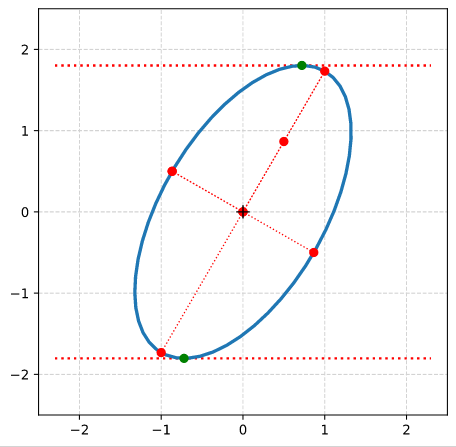
With the results above we can plot the special extremal points on our resulting ellipse ES:
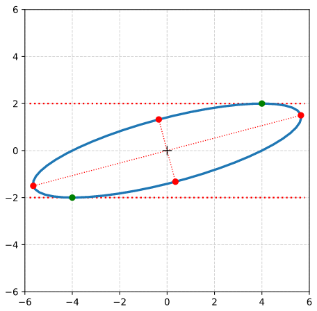
This plot reminds very much about a corresponding plot in the previous post where we sheared a circle. But note, that our present ellipse has a different shape and longer main axes. And again we can calculate the angle by which the ellipse is rotated against the x-axis.
\alpha \,=\, \arctan \left( { y_{s1} \over x_{s1} } \right) , \quad \left( \,\approx 14.9 \deg \right)
\]
I leave details to the reader. Note that the angle is different from what we got in the previous post.
Step 2: Shearing of a general centered and rotated ellipse
The ellipse above was a special one whose axes were aligned with the coordinate axes of the ECS. But also a general centered, but rotated ellipse can be represented by a quadratic form like:
\alpha_o\,x_o^2 \, + \, \beta_o \, x_o y_o \, + \, \gamma_o \, y_o^2 \:=\: \delta_o
\]
The coefficients can be regarded as elements of a symmetric matrix, which characterizes a conic section:
\pmb{\operatorname{A}}_q^O \: = \: \begin{pmatrix} \alpha_o & 1/2\, \beta_o \\ 1/2\,\beta_o & \gamma_o \end{pmatrix}
\]
with
\left(\,x_o,\, y_o\,\right) \,\circ\, \pmb{\operatorname{A}}_q^O \,\circ\, \left(\,x_o,\, y_o\,\right)^T \: = \: \delta_o
\]
The condition for an ellipse as a special case of a conic section is:
det\left(\pmb{\operatorname{A}}_q^O \right) \: \gt \: 0 \quad \Rightarrow \quad \alpha_o \, \gamma_o \,-\, {1\over4}\,\beta_o^2 \,\gt\, 0.
\]
Now, we can easily prove that a shear transformation does not change the basic form of the equation and that it preserves the determinant of the characteristic matrix. With our transformation rules we get
\alpha_o\, \left(\, x_S\,-\, \lambda_S\, y_S\, \right)^2 \, + \, \beta_o \, \left(\, x_S \,-\, \lambda_S\, y_S \,\right)\,y_S \, + \, \gamma_o \, y_S^2 \:=\: \delta_o
\]
&\alpha_o\, x_S^2 \,+\, \left(\, \beta_o \,-\, 2\,\lambda_S\, \alpha_o \, \right) \, x_S \, y_S \, + \, \left(\, \gamma_o \,-\, \lambda_S\, \beta_o \,+\, \alpha_o\,\lambda_S^2 \,\right)\, y_S^2 \:=\: \delta_o \\
\end{align}
\]
This is the regular quadratic form for a new ellipse ES with a definition matrix
\pmb{\operatorname{A}}_q^S \: = \: \begin{pmatrix} \alpha_o & 1/2\,\left(\beta_o \,-\,2 \alpha_o \lambda_S \right) \\
1/2\,\left(\beta_o \,-\,2 a_o \lambda_S \right) & \alpha_o \, \lambda_S^2 \, -\, \beta_o \lambda_S \,+\, \gamma_o \end{pmatrix}
\]
And the new determinant is:
\begin{align}
det\left( \pmb{\operatorname{A}}_q^S \right) \,&=\, \alpha_o\,\left(\alpha_o\, \lambda_S^2 \, -\, \beta_o \lambda_S \,+\, \gamma_o \right) \,-\,
{1\over 4}\,\left(\beta_o \,-\,2 \alpha_o \lambda_S \right)^2 \\
&= \, \alpha_o^2 \, \lambda_S^2 \,-\, \alpha_o\,\beta_o \, \lambda_S \,+\, \alpha_o \, \gamma_o \,-\, {1\over 4} \, \beta_o^2 \,+\, \alpha_o \, \beta_o\, \lambda_S \, -\,\ \alpha_o^2 \, \lambda_S^2 \\
&= \, \alpha_o\, \gamma_o \,-\, {1\over 4}\,\beta_o^2 \:=\: det\left( \pmb{\operatorname{A}}_q^O \right) \:\gt\: 0
\end{align}
\]
Nice, isn’t it? So it is definitely an ellipse again.
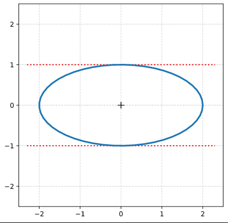
Shearing of a rotated example ellipse
Let apply these results for a concrete example ellipse, which we construct by rotating an axis-parallel ellipse with aa = 2.0 and ba = 1.0: The longer principal axis a=2.0 of the ellipse is assumed to be oriented in x-direction; in y-direction we have the shorter ellipse-axis. The points (xa, ya) on this axis-parallel ellipse fulfill
{x_a^2 \over a_a^2} \,+\, {y_a^2 \over b_a^2} \:=\: 1
\]
Now we rotate this ellipse by an angle Ψ = 60°. The resulting ellipse EO,
which we will shear in a minute, is described by the following matrix
\pmb{\operatorname{A}}_q^O \:=\:
\begin{pmatrix} \alpha_o & \beta_o / 2 \\ \beta_o / 2 & \gamma_o \end{pmatrix}
\]
with the following numerical values of its coefficients
\begin{align}
\alpha_o \:&=\: 3.25 \\
\beta_o \:&=\: -1.29903811 \\
\gamma_o \:&=\: 1.75 \\
\delta_o \:&=\: 4.0
\end{align}
\]
For details of the required formulas and calculation steps (application of scaling and rotation matrices) see here.
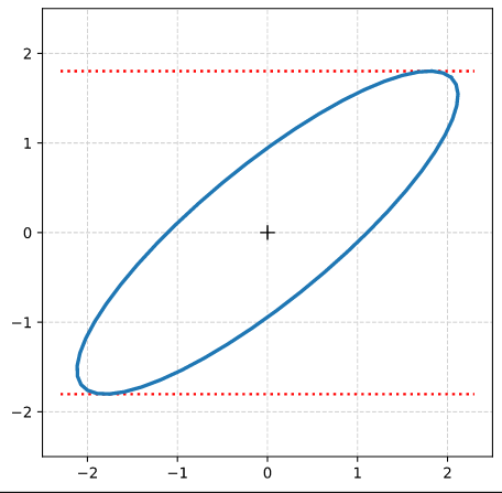
Application of the shear operation on the rotated ellipse
We now apply a shear operation with a shear parameter λS = 0.6 to our rotated example ellipse. The transformation rules for the components of the original ellipse’s position vectors of course are:
\pmb{v_o} \,=\, \begin{pmatrix} x_o \\ y_o \end{pmatrix}
\]
x_S \: &= \: x_o \, + \, \lambda_S * y_o \\
y_S \: &= \: y_o
\end{align}
\]
A plot shows that the shear operation indeed result in a new, elongated and rotated ellipse ES:
Transformation of the matrix coefficients
We repeat the quadratic equation for points of the original centered and rotated ellipse EO:
\alpha_o\,x_o^2 \, + \, \beta_o \, x_o \, y_o \, + \, \gamma_o \, y_o^2 \:=\: \delta_o
\]
For the sake of completeness we look at the coefficients of the quadratic form for ES: .
\alpha_o\, \left(\, x_S\,-\, \lambda_S\, y_S\, \right)^2 \, + \, \beta_o \, \left(\, x_S \,-\, \lambda_S\, y_S \,\right)\,y_S \, + \, \gamma_o \, y_S^2 \:=\: \delta_o
\]
Rearranging indeed leads to a new quadratic form:
&\alpha_o\, x_S^2 \,+\, \left(\, \beta_o \,-\, 2\,\lambda_S\, \alpha_o \, \right) \, x_S \, y_S \, + \, \left(\, \gamma_o \,-\, \lambda_S\, \beta_o \,+\, \alpha_o\,\lambda_S^2 \,\right)\, y_S^2 \:=\: \delta_S, \\
&\left( \operatorname{with}\: \delta_S \,=\, \delta_o\, \right)
\end{align}
\]
The coefficients \(\alpha_S \), \(\beta_S \), \(\gamma_S \) of \(\pmb{\operatorname{A}}_q^S \) and \(\delta_S \) are given by
\begin{align}
\alpha_S \:&=\: \alpha_0 \\
\beta_S \:&=\: \beta_o \,-\, 2\,\lambda_S\, \alpha_o \, \phantom{\large{)}} \\
\gamma_S \:&=\: \gamma_o \,-\, \lambda_S\, \beta_o \,+\, \alpha_o\,\lambda_S^2 \,\phantom{\large{)}} \\
\delta_S \:&=\: \delta_o
\end{align}
\]
These coefficients allow us to numerically calculate the basic geometrical properties of the new ellipse ES. As soon as you have the coefficients of the quadratic form of a transformed ellipse you (of course) also know its geometric properties. See my post series on ellipses and matrix coefficients for all required formulas that relate the geometrical properties of an ellipse to the coefficients of its defining matrix \(\pmb{\operatorname{A}}_q^S \) and the related quadratic form.
The following plot marks the coordinates of key points on the sheared ellipse. All data were calculated from the numerical values of the \(\pmb{\operatorname{A}}_q^O \)- and the \(\pmb{\operatorname{A}}_q^S \)-coefficients.
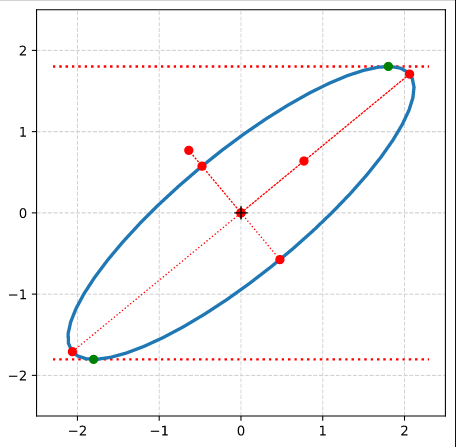
The red dots outside and inside the ellipse mark the end-points of the normalized eigenvectors of \(\pmb{\operatorname{A}}_q^S \).
The inclination angle of the major axis of ES with the x-axis of the ECS was determined to be
\psi \:=\: – 0.5 * {\pi \over 180} * \operatorname{arcsin} \left( {\beta_S \over \sqrt{\beta_S^2 + (\gamma_S – \alpha_S)^2} } \right) \:\approx\: 39.65
\]
The lengths of the new principal axes are given by
\sigma_1^S \,=\, \sqrt{\lambda_1^S} \:&=\: \sqrt{\, {1 \over 2} \left[ \, \left( \gamma_S \,+\, \alpha_S \right) \,+\, \left[ \beta^2_S \, +\, \left( \gamma_S \,-\, \alpha_S \right)^2 \, \right]^{1/2} \right] \,} \:\approx\: 0.747 \\
\sigma_2^S \,=\, \sqrt{\lambda_2^S} \:&=\: \sqrt{\, {1 \over 2} \left[ \, \left( \gamma_S \,+\, \alpha_S \right) \,-\, \left[ \beta^2_S \, +\, \left( \gamma_S \,-\, \alpha_S \right)^2 \, \right]^{1/2} \right] \,} \:\approx\: 2.678
\end{align}
\]
We are back to two (!) rotations
Let us think a bit of what we have achieved. Our perspective here is a one from a chosen static ECS whose origin coincides with the original ellipse or circle:
- Shearing of a centered circle results in a centered, rotated ellipse. We can replace the shear-operation by a sequence of an asymmetric scaling operation followed by one rotation.
- A shear operation transforms an original axis-parallel ellipse into a rotated ellipse. Again we could have replaced the operation by a scaling followed by one rotation.
- Shearing of a centered ellipse, but with axes already rotated against the coordinate-axes of the ECS, again leads to a centered ellipse, but differently scaled and rotated by a new angle against the ECS-axes. A replacement of the shear operation by simpler affine operations would have required the following steps:
- First we would have to rotate the ellipse such that its axes afterward were aligned with the ECS-axes,
- then we would scale its axes asymmetrically
- and eventually we would rotate the intermediate ellipse to its final inclination angle against the ECS-axes.
Note that we do not change the once selected ECS during these steps. Now, you could ask: Why can’t we just rotate the original ellipse into its final orientation and then scale it? Answer: A scaling of x- and y-coordinates of the points on the ellipse
x_{scale} \,= \, \eta_x \,*\, x, \quad y_{scale} \,= \, \eta_y \,*\, y
\]
by some constant factors ηx and ηy would distort the ellipse in our fixed ECS and again rotate it. Scaling of an ellipse without rotating it only works in an ECS whose coordinate axes are aligned with the ellipse’s primary axes.
Therefore a synonym formulation of what we said about shearing a general ellipse rotated against the ECS’s coordinate axes would be:
There is another ECS, lets call it ECS-PCA, which is rotated against our chosen ECS and whose coordinate axes are aligned with the primary axis of our original ellipse. In ECS-PCA the shear operation can be replaced by scaling plus one rotation.
Summary: Because as our original, rotated ellipse does not exhibit isotropy, we find that shearing in an arbitrarily chosen ECS can not be reduced to just one rotation plus scaling. One of the required rotations will correspond to a so called primary axis-transformation (PCA-transformation). The other rotation reflects the shear effect in a certain direction. Even if we had by chance chosen the specific ECS-PCA to be our working ECS we would at least have to perform one rotation.
A shear operation of a non-isotropic figure can in no ECS be reduced to just a scaling operation. We expect that this will show up in a matrix decomposition like SVD.
Conclusion
In this post we have extended the results of previous posts. Not only does the application of a shear operation on a circle produce an ellipse. We also get a centered ellipse when we apply a shear operation onto an original centered ellipse with an inclination angle against the coordinate axes of our ECS. The coefficients of the quadratic form and its related matrix, which describe the sheared ellipse, can easily be derived from the coefficients for the original ellipse and the shear parameter λ. From the resulting coefficients one can in turn determine the most relevant geometrical properties of the sheared ellipse.
In the next posts of this series we first clarify the connection between the defining matrix of the sheared ellipse with the defining matrix of the original ellipse. It is clear that the relation will be given in terms of the shear matrix Msh.
In a subsequent post we will then have a look at 3-dimensional ellipsoids and apply a shear operation to them.