
I continue my small series on a single neuron perceptron to study the positive effects of the normalization of input data in combination with the use of the sigmoid function as the activation function. In the last article
we have seen that the saturation of the sigmoid function for big positive or negative arguments can prevent a smooth gradient descent under certain conditions – even if a global minimum clearly exists.
A perceptron with just one computing neuron is just a primitive example which demonstrates what can happen at the neurons of the first computing layer after the input layer of a real “Artificial Neural Network” [ANN]. We should really avoid to provide too big input values there and take into account that input values for different features get added up.
Measures against saturation at neurons in the first computing layer
There are two elementary methods to avoid saturation of sigmoid like functions at neurons of the first hidden layer:
- Normalization: One measure to avoid big input values is to normalize the input data. Normalization can be understood as a transformation of given real input values for all of the features into an interval [0, 1] or [-1, 1]. There are of course many transformations which map a real number distribution into a given limited interval. Some keep up the relative distance of data points, some not. We shall have a look at some standard normalization variants used in Machine Learning [ML] during this and the next article .
The effect with respect to a sigmoidal activation function is that the gradient for arguments in the range [-1, 1] is relatively big. The sigmoid function behaves almost as a linear function in this argument region; see the plot in the last article. - Choosing an appropriate (statistical) initial weight distribution: If we have a relatively big feature space as e.g. for the MNIST dataset with 784 features, normalization alone is not enough. The initial value distribution for weights must also be taken care of as we add up contributions of all input nodes (multiplied by the weights). We can follow a recommendation of LeCun (1990); see the book of Aurelien Geron recommended (here) for more details.
Then we would choose a uniform distribution of values in a range [-alpha*sqrt(1/num_inp_nodes), alpha*sqrt(1/num_inp_nodes)], with alpha $asymp; 1.73 and num_inp_nodes giving the number of input nodes, which typically is the number of features plus 1, if you use a bias neuron. As a rule of thumb I personally take [-0.5*sqrt(1/num_inp_nodes, 0.5*sqrt[1/num_inp_nodes].
Normalization functions
The following quick&dirty Python code for a Jupyter cell calls some normalization functions for our simple perceptron scenario and directly executes the transformation; I have provided the required import statements for libraries already in the last article.
# ********
# Scaling
# ********

b_scale = True
scale_method = 3
# 0: Normalizer (standard), 1: StandardScaler, 2. By factor, 3: Normalizer per pair
# 4: Min_Max, 5: Identity (no transformation) - just there for convenience

shape_ay = (num_samples,)
ay_K1 = np.zeros(shape_ay)
ay_K2 = np.zeros(shape_ay)

# apply scaling
if b_scale:
    # shape_input = (num_samples,2)
    rg_idx = range(num_samples)
    if scale_method == 0:

        shape_input = (2, num_samples)
        ay_K = np.zeros(shape_input)
        for idx in rg_idx:
            ay_K[0][idx] = li_K1[idx]
            ay_K[1][idx] = li_K2[idx]
        scaler = Normalizer()
        ay_K = scaler.fit_transform(ay_K)
        for idx in rg_idx:
            ay_K1[idx] = ay_K[0][idx]
            ay_K2[idx] = ay_K[1][idx]
        print(ay_K1)
        print("\n")
        print(ay_K2)
    elif scale_method == 1:
        shape_input = (num_samples,2)
        ay_K = np.zeros(shape_input)
        for idx in rg_idx:
            ay_K[idx][0] = li_K1[idx]
            ay_K[idx][1] = li_K2[idx]
        scaler = StandardScaler()
        ay_K = scaler.fit_transform(ay_K)
        for idx in rg_idx:
            ay_K1[idx] = ay_K[idx][0]
            ay_K2[idx] = ay_K[idx][1]
    elif scale_method == 2:
        dmax = max(li_K1.max() - li_K1.min(), li_K2.max() - li_K2.min())
        ay_K1 = 1.0/dmax * li_K1
        ay_K2 = 1.0/dmax * li_K2
    elif scale_method == 3:
        shape_input = (num_samples,2)
        ay_K = np.zeros(shape_input)
        for idx in rg_idx:
            ay_K[idx][0] = li_K1[idx]
            ay_K[idx][1] = li_K2[idx]
        scaler = Normalizer()
        ay_K = scaler.fit_transform(ay_K)
        for idx in rg_idx:
            ay_K1[idx] = ay_K[idx][0]
            ay_K2[idx] = ay_K[idx][1]
    elif scale_method == 4:
        shape_input = (num_samples,2)
        ay_K = np.zeros(shape_input)
        for idx in rg_idx:
            ay_K[idx][0] = li_K1[idx]
            ay_K[idx][1] = li_K2[idx]
        scaler = MinMaxScaler()
        ay_K = scaler.fit_transform(ay_K)
        for idx in rg_idx:
            ay_K1[idx] = ay_K[idx][0]
            ay_K2[idx] = ay_K[idx][1]
    elif scale_method == 5:
        ay_K1 = li_K1
        ay_K2 = li_K2


# Get overview over costs on weight-mesh
wm1 = np.arange(-5.0,5.0,0.002)
wm2 = np.arange(-5.0,5.0,0.002)
#wm1 = np.arange(-0.3,0.3,0.002)
#wm2 = np.arange(-0.3,0.3,0.002)
W1, W2 = np.meshgrid(wm1, wm2)
C, li_C_sgl = costs_mesh(num_samples = num_samples, W1=W1, W2=W2, li_K1 = ay_K1, li_K2 = ay_K2, \
                               li_a_tgt = li_a_tgt)


C_min = np.amin(C)
print("C_min = ", C_min)
IDX = np.argwhere(C==C_min)
print ("Coordinates: ", IDX)
wmin1 = W1[IDX[0][0]][IDX[0][1]]
wmin2 = W2[IDX[0][0]][IDX[0][1]]
print("Weight values at cost minimum:",  wmin1, wmin2)

# Plots
# ******
fig_size = plt.rcParams["figure.figsize"]
#print(fig_size)
fig_size[0] = 19; fig_size[1] = 19

fig3 = plt.figure(3); fig4 = plt.figure(4)

ax3 = fig3.gca(projection='3d')
ax3.get_proj = lambda: np.dot(Axes3D.get_proj(ax3), np.diag([1.0, 1.0, 1, 1]))
ax3.view_init(25,135)
ax3.set_xlabel('w1', fontsize=16)
ax3.set_ylabel('w2', fontsize=16)
ax3.set_zlabel('Total costs', fontsize=16)
ax3.plot_wireframe(W1, W2, 1.2*C, colors=('green'))


ax4 = fig4.gca(projection='3d')
ax4.get_proj = lambda: np.dot(Axes3D.get_proj(ax4), np.diag([1.0, 1.0, 1, 1]))
ax4.view_init(25,135)
ax4.set_xlabel('w1', fontsize=16)
ax4.set_ylabel('w2', fontsize=16)
ax4.set_zlabel('Single costs', fontsize=16)
ax4.plot_wireframe(W1, W2, li_C_sgl[0], colors=('blue'))
#ax4.plot_wireframe(W1, W2, li_C_sgl[1], colors=('red'))
ax4.plot_wireframe(W1, W2, li_C_sgl[5], colors=('orange'))
#ax4.plot_wireframe(W1, W2, li_C_sgl[6], colors=('yellow'))
#ax4.plot_wireframe(W1, W2, li_C_sgl[9], colors=('magenta'))
#ax4.plot_wireframe(W1, W2, li_C_sgl[12], colors=('green'))

plt.show()
The results of the transformation for our two features are available in the arrays “ay_K1” and “ay_K2”. These arrays will then be used as an input to gradient descent.
Some
remarks on some normalization methods:
Normalizer: It is in the above code called by setting “scale_method=0”. The “Normalizer” with standard parameters scales by applying a division by an averaged L2-norm distance. However, its application is different from other SciKit-Learn scalers:
It normalizes over all data given in a sample. The dimensions beyond 1 are NOT interpreted as features which have to be normalizes separately – as e.g. the “StandardScaler” does. So, you have to be careful with index handling! This explains the different index-operation for “scale_method = 0” compared to other cases.
StandardScaler: Called by setting “scale_method=1”. The StandardScaler accepts arrays of samples with columns for features. It scales all features separately. It subtracts the mean average of all feature values of all samples and divides afterwards by the standard deviation. It thus centers the value distribution with a mean value of zero and a variance of 1. Note however that it does not limit all transformed values to the interval [-1, 1].
MinMaxScaler: Called by setting “scale_method=4”. The MinMaxScaler
works similar to the StandardScaler but subtracts the minimum and divides by the (max-min)-difference. It therefore does not center the distribution and does not set the variance to 1. However, it limits the transformed values to the interval [-1, 1].
Normalizer per sample: Called by setting “scale_method=3”. This applies the Normalizer per sample! I.e., it scales in our case both the given feature values for one single by their mean and standard deviation. This may at first sound totally meaningless. But we shall see in the next article that it is not in case for our special set of 14 input samples.
Hint: For the rest of this article we shall only work with the StandardScaler.
Input data transformed by the StandardScaler
The following plot shows the input clusters after a transformation with the “StandardScaler”:
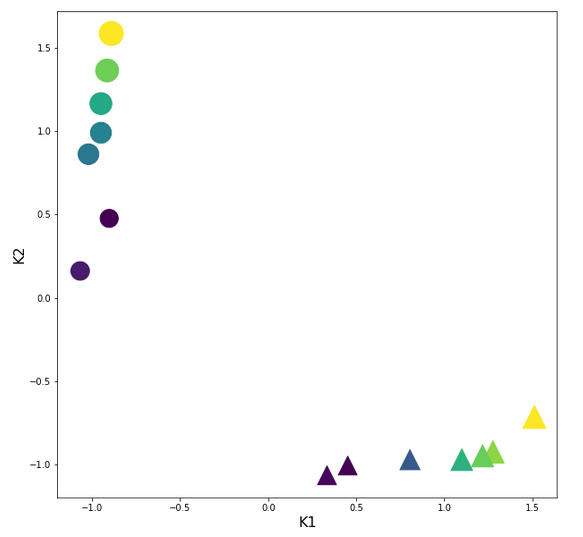
You should recognize two things: The centralization of the features and the structural consistence of the clusters to the original distribution before scaling!
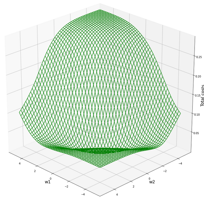
The cost hyperplane over the {w1, w2}-space after the application of the StandardScaler to our input data
Let us apply the StandardScaler and look at the resulting cost hyperplane. When we set the parameters for a mesh display to
wm1 = np.arange(-5.0,5.0,0.002), wm2 = np.arange(-5.0,5.0,0.002)
we get the following results:
C_min =  0.0006239618496774544
Coordinates:  [[2695 2259]]
Weight values at cost minimum: -0.4820000000004976 0.3899999999994064
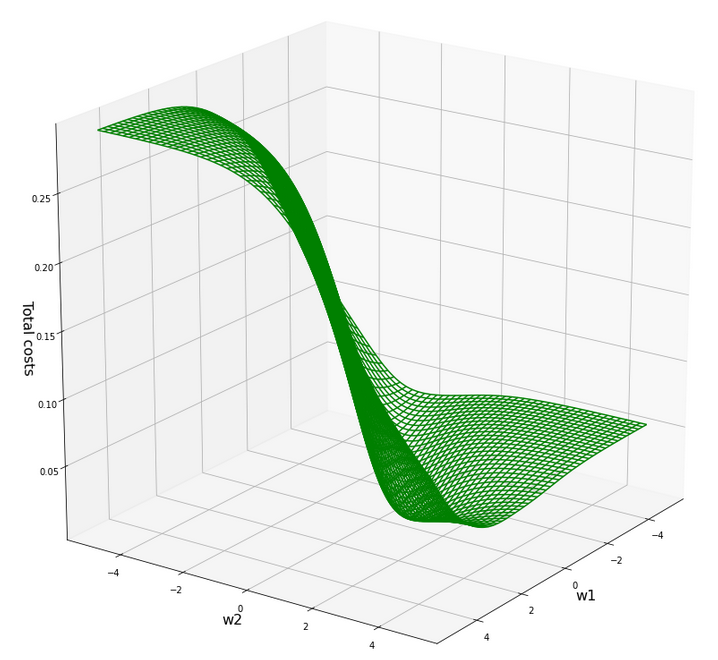
Plots for total costs over the {w1, w2}-space from different angles
Plot for individual costs (i=0, i=5) over the {w1, w2}-space
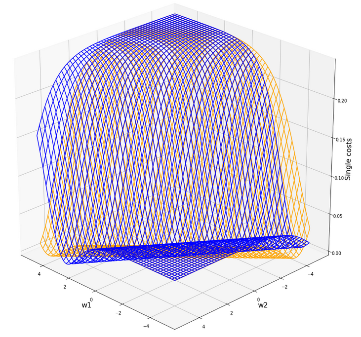
The index “i” refers to our sample-array (see the last article).
Gradient descent after scaling with the “StandardScaler”
Ok, let us now try gradient descent again. We set the following parameters:
w1_start = -0.20, w2_start = 0.25 eta = 0.1, decrease_rate = 0.000001, num_steps = 2000
Results:
Stoachastic Descent
          Kt1       Kt2     K1     K2  Tgt       Res       Err
0   1.276259 -0.924692  200.0   14.0  0.3  0.273761  0.087463
1  -1.067616  0.160925    1.0  107.0  0.7  0.640346  0.085220
2   0.805129 -0.971385  160.0   10.0  0.3  0.317122  0.057074
3  -0.949833  1.164828   11.0  193.0  0.7  0.713461  0.019230
4   1.511825 -0.714572  220.0   32.0  0.3  0.267573  0.108090
5  -0.949833  0.989729   11.0  178.0  0.7  0.699278  0.001031
6   0.333998 -1.064771  120.0    2.0  0.3  0.359699  0.198995
7  -0.914498  1.363274   14.0  210.0  0.7  0.725667  0.036666
8   1.217368 -0.948038  195.0   12.0  0.3  0.277602  0.074660
9  -0.902720  0.476104   15.0  134.0  0.7  0.650349  0.070930
10  0.451781 -1.006405  130.0    7.0  0.3  0.351926  0.173086
11 -1.020503  0.861322    5.0  167.0  0.7  0.695876  0.005891
12  1.099585 -0.971385  185.0   10.0  0.3  0.287246  0.042514
13 -0.890942  1.585067   16.0  229.0  0.7  0.740396  0.057709

Batch Descent
          Kt1       Kt2     K1     K2  Tgt       Res       Err
0   1.276259 -0.924692  200.0   14.0  0.3  0.273755  0.087482
1  -1.067616  0.160925    1.0  107.0  0.7  0.640352  0.085212
2   0.805129 -0.971385  160.0   10.0  0.3  0.317118  0.057061
3  -0.949833  1.164828   11.0  193.0  0.7  0.713465  0.019236
4   1.511825 -0.714572  220.0   32.0  0.3  0.267566  0.108113
5  -0.949833  0.989729   11.0  178.0  0.7  0.699283  0.001025
6   0.333998 -1.064771  120.0    2.0  0.3  0.359697  0.198990
7  -0.914498  1.363274   14.0  210.0  0.7  0.725670  0.036672
8   1.217368 -0.948038  195.0   12.0  0.3  0.277597  0.074678
9  -0.902720  0.476104   15.0  134.0  0.7  0.650354  0.070923
10  0.451781 -1.006405  130.0    7.0  0.3  0.351924  0.173080
11 -1.020503  0.861322    5.0  167.0  0.7  0.695881  0.005884
12  1.099585 -0.971385  185.0   10.0  0.3  0.287241  0.042531
13 -0.890942  1.585067   16.0  229.0  0.7  0.740400  0.057714

Total error stoch descent:  0.07275422919538276
Total error batch descent:  0.07275715820661666
The attentive reader has noticed that I extended my code to include the columns with the original (K1, K2)-values into the Pandas dataframe. The code of the new function “predict_batch()” is given below. Do not forget to change the function calls at the end of the gradient descent code, too.
Now we obviously can speak of a result! The calculated (w1, w2)-data are:
Final (w1,w2)-values stoch : ( -0.4816 ,  0.3908 )
Final (w1,w2)-values batch : ( -0.4815 ,  0.3906 )
Yeah, this is pretty close to the values we got via the fine grained mesh analysis of the cost function before! And within the error range!
Changed code for two of our functions in the last article
def predict_batch(num_samples, w1, w2, ay_k_1, ay_k_2, li_K1, li_K2, li_a_tgt):
    shape_res = (num_samples, 7)
    ResData = np.zeros(shape_
res)
    rg_idx = range(num_samples)
    err = 0.0
    for idx in rg_idx:
        z_in  = w1 * ay_k_1[idx] + w2 * ay_k_2[idx]
        a_out = expit(z_in)
        a_tgt = li_a_tgt[idx]
        err_idx = np.absolute(a_out - a_tgt) / a_tgt
        err += err_idx
        ResData[idx][0] = ay_k_1[idx]
        ResData[idx][1] = ay_k_2[idx]
        ResData[idx][2] = li_K1[idx]
        ResData[idx][3] = li_K2[idx]
        ResData[idx][4] = a_tgt
        ResData[idx][5] = a_out
        ResData[idx][6] = err_idx
    err /= float(num_samples)
    return err, ResData

def create_df(ResData):
    ''' ResData: Array with result values K1, K2, Tgt, A, rel.err
    '''
    cols=["Kt1", "Kt2", "K1", "K2", "Tgt", "Res", "Err"]
    df = pd.DataFrame(ResData, columns=cols)
    return df
How does the epoch evolution after the application of the StandardScaler look like?
Let us plot the evolution for the stochastic gradient descent:
Cost and weight evolution during stochastic gradient descent
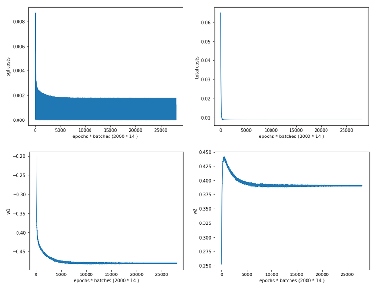
Ok, we see that despite convergence the difference in the costs for different samples cannot be eliminated. It should be clear to the reader, why, and that this was to be expected.
We also see that the total costs (calculated from the individual costs) seemingly converges much faster than the weight values! Our gradient descent path obviously follows a big slope into a rather flat valley first (see the plot of the total costs above). Afterwards there is a small gradient sideways and down into the real minimum – and it obviously takes some epochs to get there. We also understand that we have to keep up a significant “learning rate” to follow the gradient in the flat valley. In addition the following rule seems to be appropriate sometimes:
We must not only watch the cost evolution but also the weight evolution – to avoid stopping gradient descent too early!
We shall keep this in mind for experiments with real multi-layer “Artificial Neural Networks” later on!
And how does the gradient descent based on the full “batch” of 14 samples look like?
Cost and weight evolution during batch gradient descent
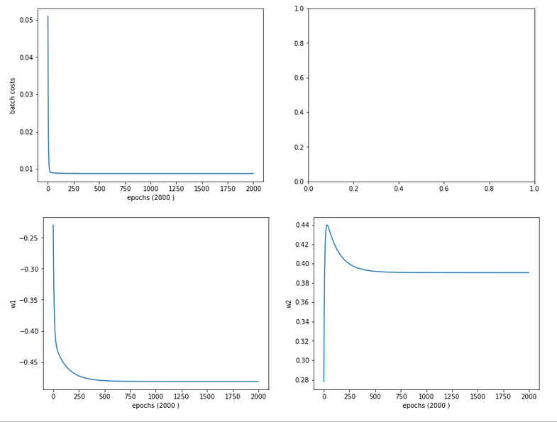
A smooth beauty!
Contour plot for separation curves in the {K1, K2}-plane
We add the following code to our Jupyter notebook:
# ***********
# Contours
# ***********

from matplotlib import ticker, cm

# Take w1/w2-vals from above w1f, w2f
w1_len = len(li_w1_ba)
w2_len = len(li_w1_ba)
w1f = li_w1_ba[w1_len -1]
w2f = li_w2_ba[w2_len -1]

def A_mesh(w1,w2, Km1, Km2):
    kshape = Km1.shape
    A = np.zeros(kshape)

    Km1V = Km1.reshape(kshape[0]*kshape[1], )
    Km2V = Km2.reshape(kshape[0]*kshape[1], )
    # print("km1V.shape = ", Km1V.shape, "\nkm1V.shape = ", Km2V.shape )

    KmV = np.column_stack((Km1V, Km2V))

    # scaling trafo
    KmT = scaler.transform(KmV)

    Km1T, Km2T = KmT.T
    Km1TR = Km1T.reshape(
kshape)
    Km2TR = Km2T.reshape(kshape)
    #print("km1TR.shape = ", Km1TR.shape, "\nkm2TR.shape = ", Km2TR.shape )

    rg_idx = range(num_samples)
    Z      = w1 * Km1TR + w2 * Km2TR
    A = expit(Z)
    return A

#Build K1/K2-mesh
minK1, maxK1 = li_K1.min()-20, li_K1.max()+20
minK2, maxK2 = li_K2.min()-20, li_K2.max()+20
resolution = 0.1
Km1, Km2 = np.meshgrid( np.arange(minK1, maxK1, resolution),
                        np.arange(minK2, maxK2, resolution))

A = A_mesh(w1f, w2f, Km1, Km2 )

fig_size = plt.rcParams["figure.figsize"]
fig_size[0] = 14
fig_size[1] = 11
fig, ax = plt.subplots()
cmap=cm.PuBu_r
cmap=cm.RdYlBu
#cs = plt.contourf(X, Y, Z1, levels=25, alpha=1.0, cmap=cm.PuBu_r)
cs = ax.contourf(Km1, Km2, A, levels=25, alpha=1.0, cmap=cmap)
cbar = fig.colorbar(cs)
N = 14
r0 = 0.6
x = li_K1
y = li_K2
area = 6*np.sqrt(x ** 2 + y ** 2)  # 0 to 10 point radii
c = np.sqrt(area)
r = np.sqrt(x ** 2 + y ** 2)
area1 = np.ma.masked_where(x < 100, area)
area2 = np.ma.masked_where(x >= 100, area)
ax.scatter(x, y, s=area1, marker='^', c=c)
ax.scatter(x, y, s=area2, marker='o', c=c)
# Show the boundary between the regions:
ax.set_xlabel("K1", fontsize=16)
ax.set_ylabel("K2", fontsize=16)
This code enables us to plot contours of predicted output values of our solitary neuron, i.e. A-values, on a mesh of the original {K1, K2}-plane. As we classified after a transformation of our input data, the following hint should be obvious:
Important hint: Of course you have to apply your scaling method to all the new input data created by the mesh-function! This is done in the above code in the “A_mesh()”-function with the following lines:
    # scaling trafo
    if (scale_method == 3):
        KmT = scaler.fit_transform(KmV)
    else:
        KmT = scaler.transform(KmV)
We can directly apply the StandardScaler on our new data via its method transform(); the scaler will use the parameters it found during his first “scaler.fit_transform()”-operation on our input samples. However, we cannot do it this way when using the Normalizer for each individual new data sample via “scale_method =3”. I shall come back to this point in a later article.
The careful reader also sees that our code will, for the time being, not work for scale_method=0, scale_method=2 and scale_method=5. Reason: I was too lazy to write a class or code suitable for these normalizing operations. I shall correct this when we need it.
But at least I added our input samples via scatter plotting to the final output. The result is:
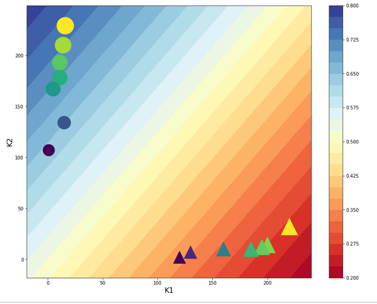
The deviations from our target values is to be expected. With a given pair of (w1, w2)-values we cannot do much better with a single neuron and a linear weight impact on the input data.
But we see: If we set up a criterion like:
- A > 0.5 => sample belongs to the left cluster,
- A ≤ 0.5 => sample belongs to the right cluster
we would have a relatively good classificator available – based on one neuron only!
Intermediate Conclusion
In this article I have shown that the “standardization” of input data, which are fed into a perceptron ahead of a gradient descent calculation, helps to circumvent problems with the saturation of the sigmoid function at the computing neuron following the input layer. We achieved this by applying the ”
StandardScaler” of Scikit-Learn. We got a smooth development of both the cost function and the weight parameters during gradient descent in the transformed data space.
We also learned another important thing:
An apparent convergence of the cost function in the vicinity of a minimum value does not always mean that we have reached the global minimum, yet. The evolution of the weight parameters may not yet have come to an end! Therefore, it is important to watch both the evolution of the costs AND the evolution of the weights during gradient descent. A too fast decline of the learning rate may not be good either under certain conditions.
In the next article
A single neuron perceptron with sigmoid activation function – III – two ways of applying Normalizer
we shall look at two other normalization methods for our simplistic scenario. One of them will give us an even better classificator.
Stay tuned and remain healthy …
And Mr Trump:
One neuron can obviously learn something about the difference of big and small numbers. This leads me to two questions, which you as a “natural talent” on epidemics can certainly answer: How many neurons are necessary to understand something about an exponential epidemic development? And why did it take so much time to activate them?