This post series studies the (in-) ability of a trained Autoencoder [AE] to create reasonable human face images from statistical vectors placed in its latent space. In my last post
Autoencoders and latent space fragmentation – I – Encoder, Decoder, latent space
I have described what the purposes of the two sub-networks of an AE, i.e. the Encoder and the Decoder, are. We saw that the so called latent space plays an important role for the interplay of these sub-networks: Vectors in the latent space – z-points – encode properties of objects presented to the Autoencoder, more precisely to its Encoder. The bunch of objects used during training thus gives us a distribution of vectors and respective z-points within certain regions of the latent space. The Decoder reconstructs objects from latent vectors.
One of my eventual objectives in this series is the creation of new objects of the same class presented to the AE during its training. I focus on the special case of images displaying human faces. Therefore, I have trained a convolutional AE with the so called CelebA dataset. After training one may hope that an AE will be able to produce images with new faces, which are not present in CelebA, when we feed the Decoder with suitable z-points. The question is what “suitable z-points” are and where they are located in the latent space.
Of course, I want to use the Decoder’s reconstruction abilities to achieve my goal. To get new faces, a statistical element is a must. The basic idea is to use statistically created z-points as input for the Decoder.
Objective of this post
In the first post of this series I have already indicated that not all vectors in the AE’s latent space may lead to the production of reasonable images. It might well be that we must hit certain confined regions of the latent space. An interesting question, therefore, is the following:
Are all generators of statistical vectors suitable to hit the regions of a latent space which an Autoencoder will fill for certain training objects?
In this and further posts I want to show you that this is not the case. A bad choice of a statistical generating method in combination with the high number of latent space dimensions may lead to a complete failure.
To achieve this insight we must study both the real z-point distribution which an AE creates for CelebA images and the artificial vector or z-point distribution coming from a specific statistical generator. In this post I study a generator which assigns the vector components values which are taken from a real number interval with a constant probability. The number of dimensions N of the latent space shall be N=256.
We shall see that we indeed get confronted with a special side of the curse of high dimensionality and that our artificial z-point distribution does not match the real one for CelebA at all if we do not restrict parameters in a somewhat counter-intuitive way. As a side effect we will learn that our AE organizes the latent vector distributions for CelebA images via functions very similar to Gaussians. Furthermore, we shall see that we speak of just one coherent and confined z-point region with very small extensions. The center of this region sits close to a hypervolume spanned by only a few (out of 256) coordinate axes.
Methods to create statistical z-points
To create statistical z-points in a latent space we have to employ some generating mechanism for respective statistical vectors. See my first post for the correspondence of z-points to latent vectors. There are multiple ways available to create latent vectors. I just name 3 popular ones:
- Create a dense homogeneous distribution by filling some volume around the origin with a grid of points.
- Use a constant probability density for values in a real number interval [-b, b], pick such values statistically and assign them to individual vector components.
- Use one or multiple Gaussian distributions to define the vector component values.
Note that when applying the second and the third method the statistics works on the level of the vector components. These components are handled as independent variables, each obeying a certain probability distribution of assignable real values.
A small calculation shows that method 1 will not work in practice, as such a distribution requires an enormous number of points for high dimensions and a decent resolution. Method 2 looks simple and works well in 2D- and 3D-spaces. The third method requires assumptions about the mean values and standard deviations to take – per vector coordinate.
Therefore it is tempting to use method 2 to create one or more artificial statistical distribution of random vectors in the latent space. This is exactly what we will try in this post – in the hope that a significant part of the resulting points will hit regions which give us reasonable images.
If you are interested in mathematical properties of vector distributions created by method 2 in multi-dimensional spaces, you will find them in the following posts of this blog:
Latent spaces – pitfalls of distributing points in multi dimensions – I – constant probability density per dimension
Latent spaces – pitfalls of distributing points in multi dimensions – II – missing specific regions
Why must we hit specific regions of the latent space?
Experience tells us that we will not get reasonable images from arbitrarily and randomly placed z-points in the latent space.. (Concrete examples will be given in the next post.) What could a plausible reason be?
Convolutional networks [CNNs] extract patterns and save them in parameters of their layer filters (or neural maps). In another post series I have shown such elementary patterns, which the innermost convolutional layers react sensitively to, for the simple case of MNIST. Patterns correspond to correlations between constituting elements of the objects we present to the neural networks. Such patterns reflect certain features of the objects. The number of elementary patterns a CNN can handle depends on the number of available kernel filters – which is fixed by the network structure. For a trained convolutional Autoencoder it is therefore reasonable to assume that a latent space vector encodes a prescription for the superposition of certain elementary patterns by which the Decoder eventually creates an image. The information for the pattern mixture is encoded both by the length and angles of latent vectors. The latter with respect to the many coordinate axes; the multitude of angles describes the orientation of a latent vector in its multi-dimensional space.
It is clear that not all prescriptions for a mixture of elementary patterns will reflect the real pixel correlations of a human face in front of some background. We must therefore assume that the latent space regions filled by a trained AE-Encoder for the training objects are the ones which give us reasonable Decoder results. In principle we could find multiple such regions in different parts of the latent space. They could have particular locations and could be confined to a relatively small volume. Therefore, we should really check that at least a part of our statistical vectors points to those regions.
Number distributions for vector components
A priori we do not know anything about the shape of z-point distribution which an Autoencoder will create in its latent space for CelebA data. Therefore, we need to get an overview over some properties of such a z-point distribution. As multidimensional spaces with a high number of dimensions like N ≥ 256 can not be presented in 3D, we need some other kind of visualization. What we shall use is a kind of spectral display for the coordinate values of our vectors:
We are going to analyze the number distribution for the values of each of the vector components.
I.e., we count the numbers of latent vectors which have values for a certain component in a series of sampling intervals for real values. We do this for all components and for a reasonable total range of values. Note that a distribution for a specific component is a one-dimensional function over ℜ.
Below we will first derive the component related distributions from real Autoencoder vectors for CelebA images. This will tell us already a lot about the orientation, the off-center location and the extensions of the real z-point distribution for CelebA.
Afterward, we will compare the CelebA specific distributions to the number distributions for artificial statistical vector distributions created by method 2.
Number distributions for vector lengths
Another nice and simple method to analyze the compatibility of vector distributions is to compare the number distributions for the vector lengths. For an orthogonal coordinate system of the latent space we can compute the length of a multi-dimensional vector by an Euclidean L2-norm. We will compare the number distribution for the lengths of latent CelebA vectors with the distribution for the lengths of vectors created by method 2. We will call the length of a vector also its “radius”.
Network setup
The basic layer structure of my AE was described already in the last post. It is relatively simple. I employ only a few Encoder and Decoder layers. I have ensured the Encoder and Decoder are actually able to solve the basic task of encoding and decoding data of real CelebA images.
We look at the results of two AE networks which differ in the number of convolutional kernel filters used:
- Test case I: We use 4 Conv2D layers in the Encoder with 32, 64, 128, 256 filters and 4 TransposeConv2D layers in the Decoder with 256, 128, 64, 32 filters, respectively.
- Test case II: We use 4 Conv2D layers in the Encoder with 64, 64, 128, 128 filters and 4 TransposeConv2D layers in the Decoder with 128, 128, 64, 64 filters, respectively.
This is reflected in the following code snippet. There you also get information on the kernel sizes, strides and padding-methods. The number of dimensions of the latent space is N = z_dim = 256. The activation function is a chosen to be Leaky Relu.
        # Test case I
        AE1 = Autoencoder(
            input_dim                  = INPUT_DIM
            , encoder_conv_filters     = [32,64,128,256]       # We take a bit bigger than D. Foster
            , encoder_conv_kernel_size = [3,3,3,3]
            , encoder_conv_strides     = [2,2,2,2]
            , encoder_conv_padding     = ['same','same','same','same']

            , decoder_conv_t_filters     = [128,64,32,n_ch]    # !!! n_ch = 1 or 3
            , decoder_conv_t_kernel_size = [3,3,3,3]
            , decoder_conv_t_strides     = [2,2,2,2]
            , decoder_conv_t_padding     = ['same','same','same','same']
            , z_dim = 256
            , act   = 0                  # activation 0:Leaky ReLU (standard), 1: ReLU, 2: SELU
        )
        # test case II
        AE2 = Autoencoder(
            input_dim                  = INPUT_DIM
            , encoder_conv_filters     = [64,64,128,128]       # We take a bit bigger than D. Foster
            , encoder_conv_kernel_size = [5,5,3,3]
            , encoder_conv_strides     = [2,2,2,2]
            , encoder_conv_padding     = ['same','same','same','same']

            , decoder_conv_t_filters     = [128,64,64,n_ch]    # !!! n_ch = 1 or 3
            , decoder_conv_t_kernel_size = [3,3,5,5]
            , decoder_conv_t_strides     = [2,2,2,2]
            , decoder_conv_t_padding     = ['same','same','same','same']
            , z_dim = 256
            , act   = 0                  # activation 0:Leaky ReLU (standard), 1: ReLU, 2: SELU
        )
A method to analyze the vector distribution in a high-dimensional vector space
The components of our latent vectors determine their angle and length. We base our analysis of corresponding z-points on the number distribution per component-value. To do this we select a suitable real value interval covering all the values for vector components which the AE actually uses. We divide this interval into a series of sufficient sub-intervals for data sampling. In our case around 100 sub-intervals.
After training of our AE we once again feed all training objects (in our case > 170,000 CelebA images) into the Encoder and keep the vectors in some Numpy arrays. Then we look at a specific component and a sampling interval and count the number of vectors for which the component value resides inside the sampling interval. Repeating this for all components and intervals we get a number distribution which can be plotted. If we are lucky the resulting shapes of the number distributions will give us information about the corresponding shape of the multi-dimensional regions which the AE fills for CelebA images.
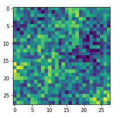
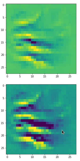
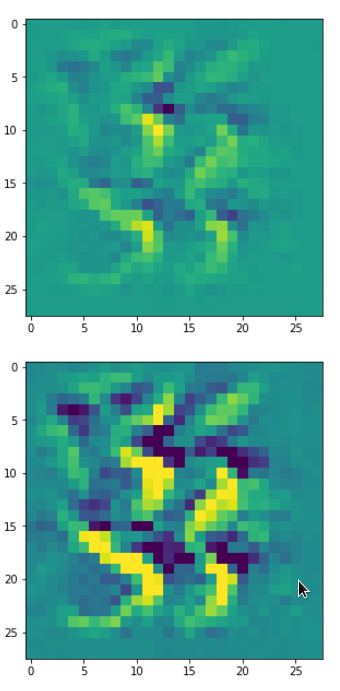
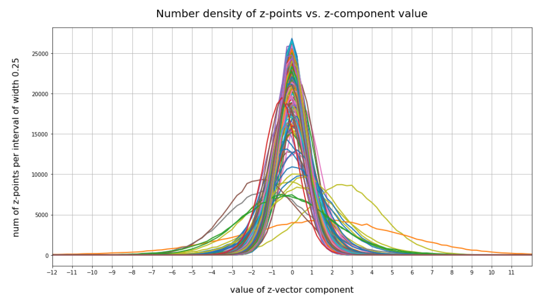
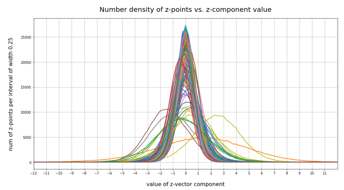
CelebA images: Number distribution for component values of latent vectors
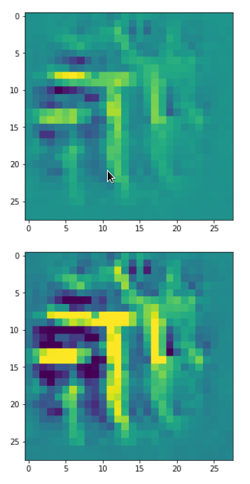
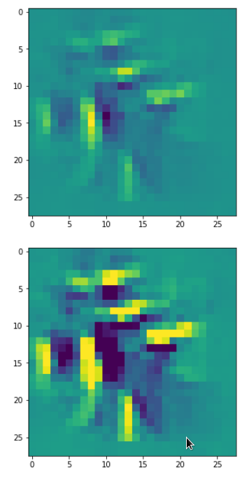
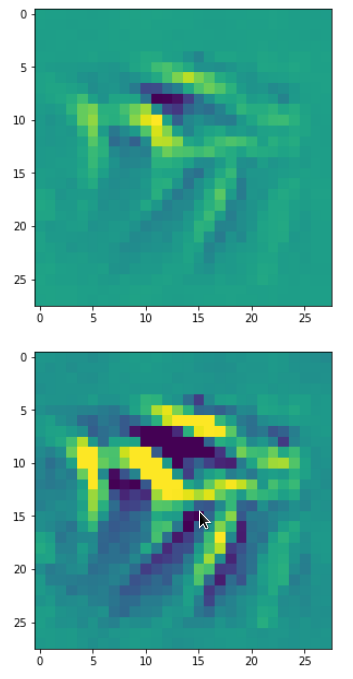
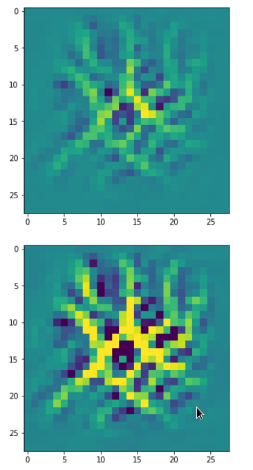
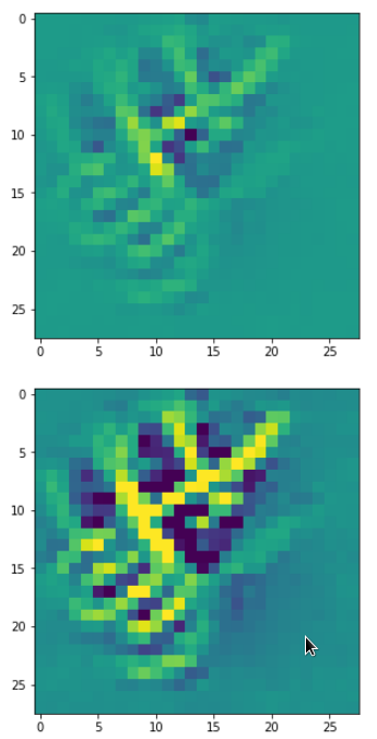
The following plot shows the number distributions for all of the 256 components of vectors for CelebA images in our trained AE’s latent space:
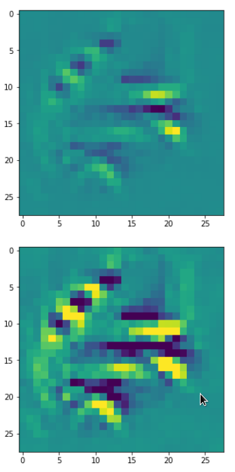
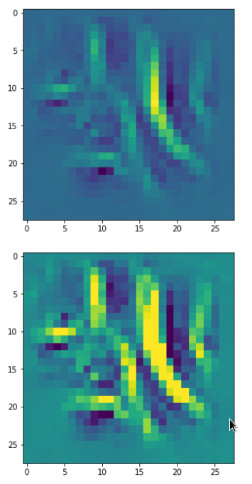
Case I: Number distribution after 24 epochs
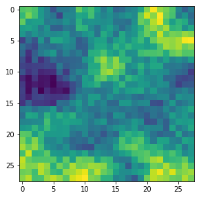
Case I: Selected components
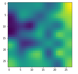
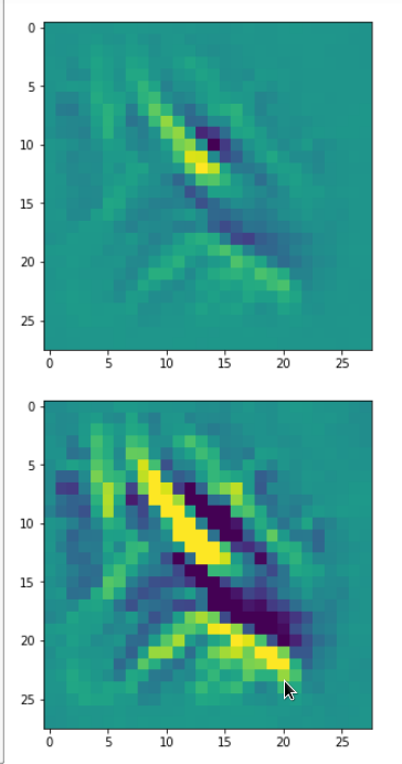
Case II: Number distribution after 30 epochs
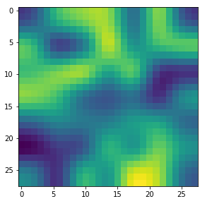
Case II: Selected components
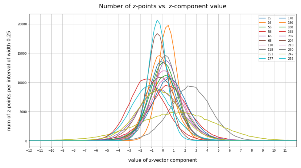
We see that the individual number distributions are very similar to Gaussian distributions. For test case II I also give you the values for the central average value μ (named mu in the list below) and the half-width (named hw below) of the most interesting components. The half-width is the difference between those coordinate values where the distribution function achieves a value of half of the maximum number value at μ:
 15 mu : -0.25 :: hw:  1.5
 16 mu :  0.5  :: hw:  1.125
 56 mu :  0.0  :: hw:  1.625
 58 mu :  0.25 :: hw:  2.125
 66 mu :  0.25 :: hw:  1.5
 68 mu :  0.0  :: hw:  2.0
110 mu :  0.5  :: hw:  1.875
118 mu :  2.25 :: hw:  2.25
151 mu :  1.5  :: hw:  4.125
177 mu : -1.0  :: hw:  2.25
178 mu :  0.5  :: hw:  1.875
180 mu : -0.25 :: hw:  1.5
188 mu :  0.25 :: hw:  1.75
195 mu : -1.5  :: hw:  2.0
202 mu : -0.5  :: hw:  2.25
204 mu : -0.5  :: hw:  1.25
210 mu :  0.0  :: hw:  1.75
230 mu :  0.25 :: hw:  1.5
242 mu : -0.25 :: hw:  2.375
253 mu : -0.5  :: hw:  1.0
These components obviously have either a relatively large absolute μ-value or a relatively large half-width. I call these components the dominant ones.
Interpretation of the number distributions per vector component
The first thing these plots prove is the fact that the results for different networks are different, too. Without proving it, I also say from experience that even two different training runs for one and the same AE network structure may result in somewhat different number distributions. But although there are some differences there are also striking similarities:
- Most of the components show a Gaussian like number distribution about some mean value.
- The mean coordinate value μ for most of the components (≥ 90%) is zero or close to it.
- The component values cover a region of [-12, 12] in our specific case.
- There are only a few components ( ≤ 25) with mean values <μ> ≥ 0.25 or <μ> ≤ -0.25.
- There are only a few components ( ≤ 10) with mean values <μ> ≥ +1.0 or <μ> ≤ -1.
- There are only relatively few components (≤ 40) with a half-width ≥ 1.
- There are only a few components (≤ 20) with a half-width ≥ 1.5
- There are only very few components ≤ 5 with a half-width ≥ 3.
A bit of thinking and imagination tells us that the center of the distribution must be located somewhat off the origin, but very close to or within a hypervolume spanned by only a few dominant coordinate axes. The multi-dimensional region filled by the z-points has significant anisotropic extensions or elongations around its center only in a few directions of the multidimensional space.
All in all we speak about a very specific, limited multi-dimensional region, located at some distance from the origin (but not too far) with a center point close to or within a sub-volume of very low dimensions spanned by some coordinate axes. The overall direction of the center with respect to the origin is well defined by a few coordinates. The diameters of the regions are small in most directions. The z-points concentrate strongly towards the center of this region. Significant diameters around the center are only given in some particular directions. The respective axes involved are less than 10% of the total number.
This also means that a primary component analysis of the z-point distribution should only give us a number of dominant main components in the same number region (0.1 * N). See forthcoming posts for such an analysis.
Analogon in 3D: In an analogous case within a 3-dimensional space we would speak of a kind of ellipsoid with a significant diameter beyond 1 only in a specific direction and a center located close to a line in a plane spanned by 2 of the 3 coordinate axes.
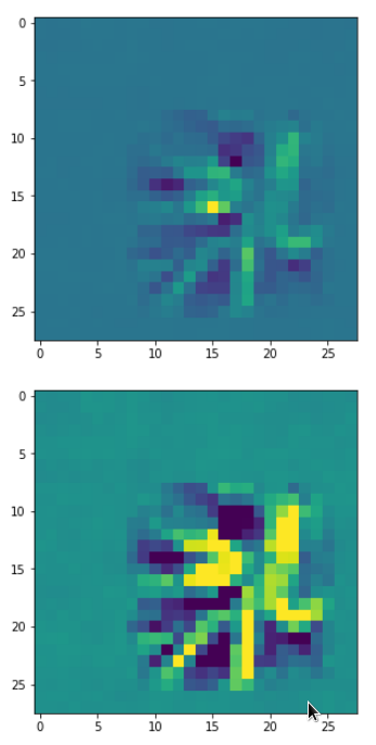
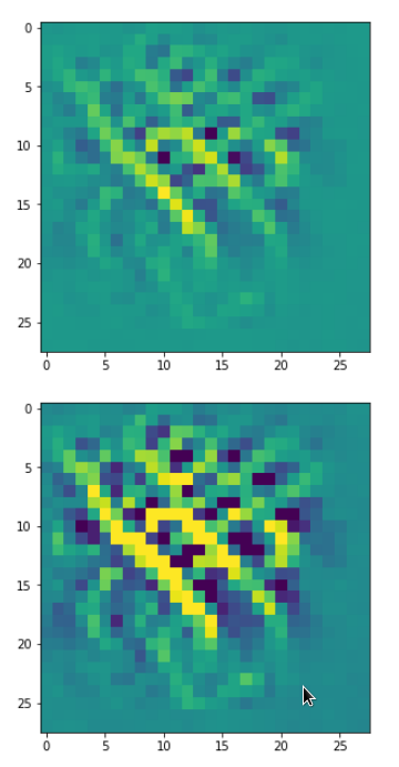
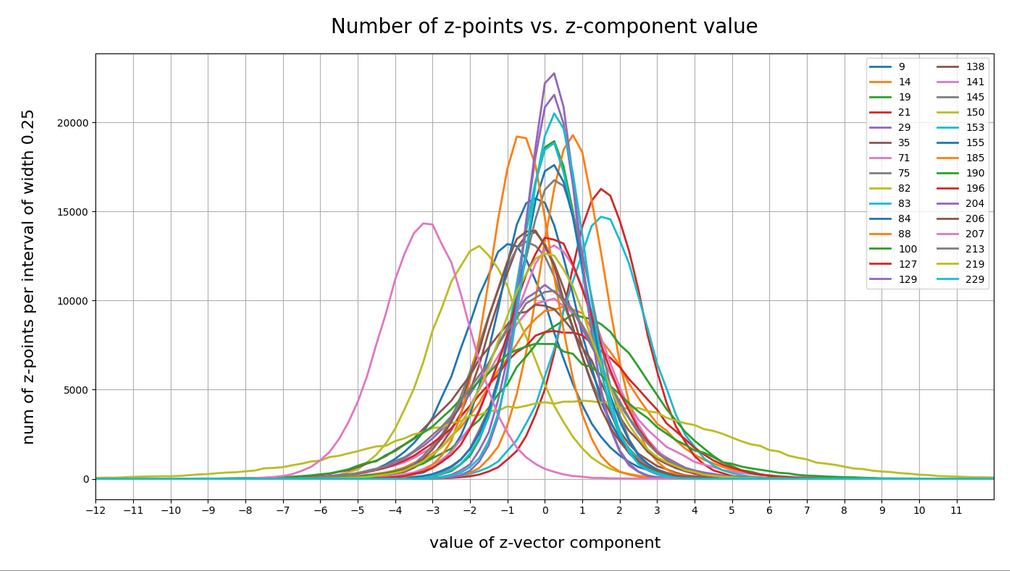
Comparison to the number distribution for statistically created vectors with a constant probability for component values in a specific interval
Now we look at the number distributions for all components of 200,000 vectors created by our method 2. We choose the same region for values [-12, 12] as displayed for our test cases I and II above. The following plot confirms what you certainly have already guessed:
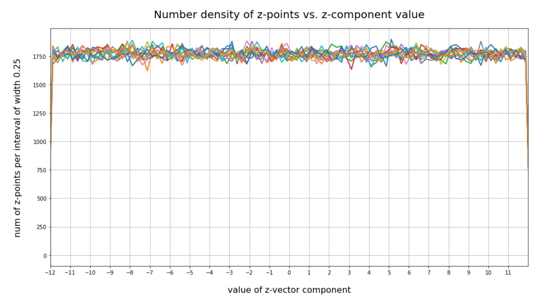
This plot just reflects the design of our probability distribution for each of the components. But the plot also indicates clearly that most of our statistically created points will not hit the latent space region which is filled by the Autoencoder for CelebA data.
The statistics obviously plays against us
It is very instructive to write a small program which scans all of the artificially created vectors and checks whether their end points lie within the region defined by the real CelebA points. I leave this to the reader. To get a good guess I personally defined a region of three times the half-width left and right of each component value center of the real distribution. The number of points fulfilling all criteria for our CelebA region came out to be exactly zero. Even with 12 times the half-width you get only very few vectors pointing into the CelebA region (around 20 vectors). Why is this the case?
The curse of a high dimensionality and a constant probability distribution
The first point is that for some components of the CelebA vectors the half-width really is rather small. So you do not cover the whole value interval [-12, 12] for the component values, but only around 75% for 12 times the half-width. Let us assume that this is the case for 7 to 8 components. Let us further assume that another 50 components the width is 90%. Then the probability to get a point is (0.75)8 * 0.965 ≈ 0.1 * 0.0018 ≈ 0.00018. This gives us only 30 out of 170,000 vectors potentially fulfilling our conditions. We are in that range.
But we know already that 90% of all components should hit an interval [-3,3]. The probability for this in the case of our method 2 is 0.25 per component. The probability for a hit thus is 0.25220 which is zero for all practical purposes. This is it what really kills our efforts to place a point in the most interesting regions of the latent space with the help of method 2 and seemingly fitting values of b.
Now, you may think: A decisive parameter for method 2 ist the interval [-b, b] from which I pick my statistical component values. What if we diminish b? E.g. to b=3 or b=2? This is a good idea as we shall see in the next paragraph. Yet, you still get only a few vectors (< 10) fulfilling all criteria for two times the half-width.
Let us reduce our b-interval to [-3, 3] for vector creation. Then for a typical vector more than 50 components miss the target region. Test runs show that even for [-2, 2] only around 10 out of 170.000 vectors would hit (outer parts) of the target region for CelebA images. In this case the few components which have off-center mu values seemingly work against us.
Things change dramatically for b=1.5 and 2 times the half-width. Now the components of all the artificial vectors fulfill our criteria. If you, however, change the intervals to hit to 1.5 times the half-width you are back again to only a very few vectors (< 10). For b=1 and 1.5 times the half-width we get again a number of 170,000 vectors fulfilling our criteria.
Why does this happen? And does it mean that when we restrict our component values to [-1.5, 1.5] we would cover our real CelebA distribution?
Number distributions for the vector lengths
Below you find a plot showing the number distribution with respect to typical vector lengths – both for CelebA (in red) and vectors artificially created with method 2 (other colors).
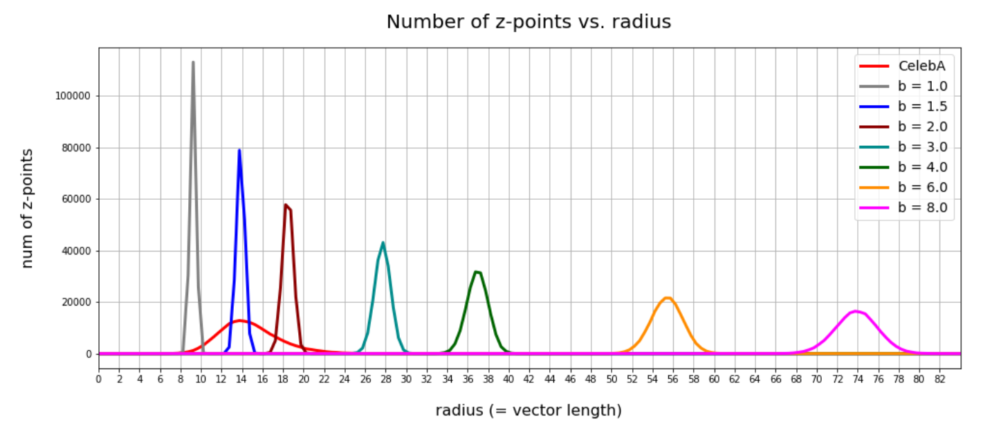
The parameter “b” of our artificial distributions defines the interval [-b, b] from which we pick component values. The probability density is a constant for this interval.
The first point you may dwell upon is the fact that the radius values get so big – much bigger than b. This is due to the high number of dimensions; see the posts named for a mathematical cover of method 2.
The second counter-intuitive point may be the following: One expects that b=12 should really be a reasonable parameter value for method 2 to cover the range of component values for CelebA. But already for b=3 or b=4 we get vectors outside the vector length interval which CelebA latent vectors fill. The reason for this are properties of the artificial radius distributions which can be derived mathematically. A mathematical calculation of the expectation value for the mean length (= radius R) of our artificially generated vectors gives us a value around
<R> ≈ b * sqrt(1/3 * N) * sqrt( 1 / (1 + 1/(4*N) )
with a relatively very narrow spread. See the derivation in the posts quoted above. sqrt in the formula above stands for the square root. The standard deviation Δstd(R) has a size of approximately
Δstd(R) ≈ b * sqrt(1/15 * N) * sqrt( 1 + 1/(4*N) )
The ratio of the half-width to radius thus declines with the square root of the number of dimensions N. As we see, only the artificial distributions for b=1, b=1.5, b=2 cover parts of the radius distribution for latent CelebA vectors.
So, if we want to use method 2 then we should work with b-values 1.0 ≤ b ≤ 2.0 to get a probability > 0 for creating reasonable images of human faces.
Will a proper value of b guarantee us reasonable face images?
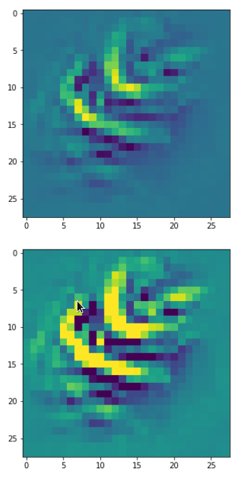
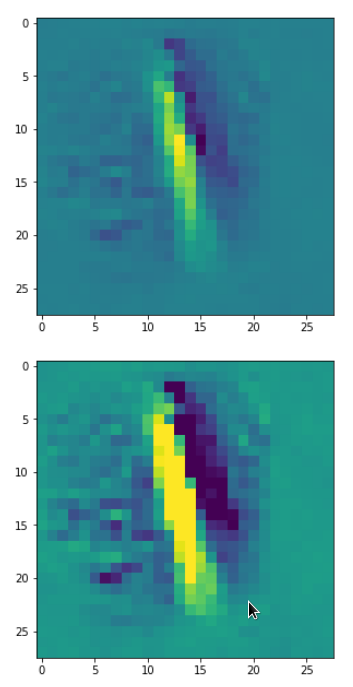
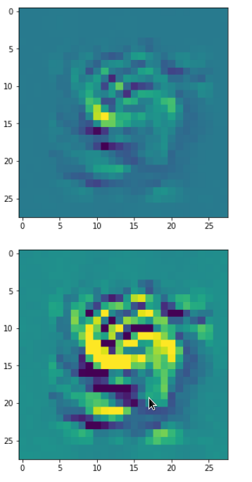
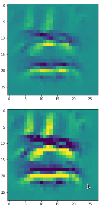
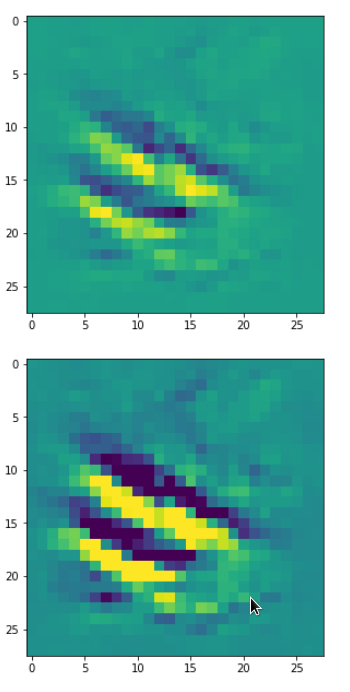
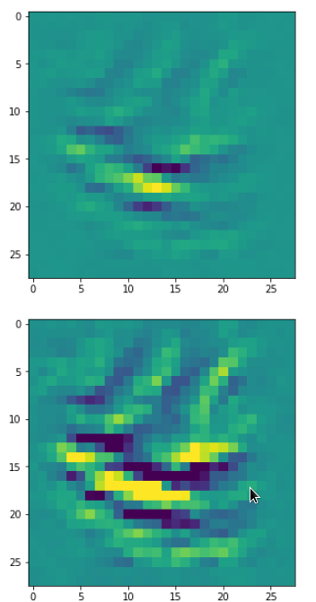
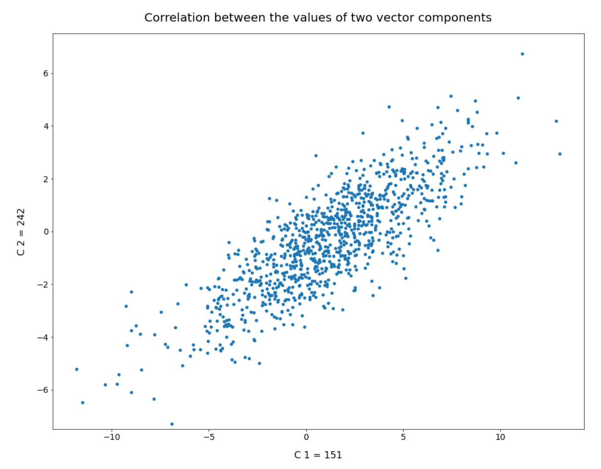
We have seen that b must be reduced to a range 1.0 ≤ b ≤ 2.0 to get reasonable radius values of our statistical vectors. Unfortunately, this does not guarantee us proper images either. The reason is that there might be correlations between the dominant component values which our simple number distributions do not reveal. We will take care of this in the next post. For now I just show you a plot of the correlation between two specific dominant components for 1000 randomly selected CelebA latent vectors:
Conclusion
In this post we have partially analyzed the distribution of vectors and related z-points which an Autoencoder creates for CelebA images in its latent space. We have found that the number distributions per vector component look like Gaussian distributions. While most of the components have a small spread around the value zero, there are a few dominant components which determine the (off-center) location and orientation of a coherent, confined and ellipsoidally shaped region for CelebA z-points. The center of this region is close to a hypervolume defined by a few axes.
It was a bit counter-intuitive to see that a simple method to create statistical z-points via a constant probability distribution for individual component values would obviously miss the relevant latent region for CelebA images totally. We saw that we would need very special parameter values to limit the component values to get artificial latent vectors with the required length. These findings alone make it very improbable that arbitrary z-points created without some restrictions for their component values would lead to reasonable face image creation by the Decoder.
Something that we have not yet covered is the question of correlations between vector components. This is the topic of the next post:
Autoencoders and latent space fragmentation – III – correlations of latent vector components