This post requires Javascript to display formulas!

In this post series I discuss results of a private study about some simple statistical vector distributions in multi-dimensional latent vector spaces. Latent spaces often appear in Machine Learning contexts and can be represented by the ℜ^N. My main interest is:

What kind of regions of such a space may we miss by choosing a vector distribution based on a simple statistical creation process?

This problem is relevant for statistical surveys of extended regions in latent vector spaces which were filled by encoding or embedding Neural Networks. A particular reason for such a survey could be the study of the reaction of a Decoder to statistical vectors in an Autoencoder’s latent space. E.g. for creative purposes. During such surveys we want to fill extended regions of the latent space with statistical data points. More precisely: With points defined by vectors reaching out from the origin. The resulting point distribution does not need to be a homogeneous one, but it should cover the whole target volume somehow and should not miss certain sub-regions in it.

Theoretically derived results for a uniform probability distribution per vector component

In my last post

Latent spaces – pitfalls of distributing points in multi dimensions – I – constant probability density per dimension

I derived some formulas for central properties of a very simple statistical vector distribution. We assumed that each component of the vectors could be created independently and with the help of a uniform, constant probability distribution: Each vector component was based on a random value taken from a defined real number interval [-b, b] with a constant and normalized probability density. Obviously, this process treats the components as statistically independent variables.

Resulting vector end points fill a quadratic area in a 2D-space or a cubic volume in 3D-space relatively well. See my last post for examples. The formulas revealed, however, that the end points of our vectors lie within a multi-dimensional spherical shell of an average radius <R>. This shell is relatively broad for small dimensions (N=2,3). But it gets narrower and narrower with a growing number of dimensions N ≥ 4.

In this post I will first test my formulas and approximations for a constant probability density in [-b, b] with the help of a numerical experiment. Afterward I discuss what kind of regions in a latent space we may miss even when we fill a sequence of growing cubes around the origin with statistical points based on our special vector distribution.

Formulas

We create vectors in a N-dimensional cube around the origin of the coordinate system of our latent vector space. The cube shall have a side-length of 2b:

The normalized probability density per dimension then simply is

ρ = 1/2 * b within [-b, b].

For details see my last post. As we use an orthogonal coordinate system the vector length, which we call radius R below, is defined in an Euclidean way by a L2-norm (square root of the sum of its squared component values).

In the last post we derived the following formulas for expectation values, variances and standard deviations of R² and R:

First order approximation to the mean radius <R> of the generated vectors

Second order approximation to the mean radius <R> of the generated vectors

First order approximation of the ratio of standard deviation for R to mean <R>

Second order approximation of the ratio of standard deviation for R to mean <R>

First order approximation of the variance of R

Second order approximation of the variance of R

In addition I give a useful approximation for the expectation value of (| R – <R> |) :

One million vectors in a multi-dimensional cube

To confirm the validity of the above approximations I created one million statistical vectors in a cube with side-length 2b for different values of N. The statistical number creation function I used in my Python3/Numpy programs was

np.random.uniform(-b, b, size = (int(1.e6), N))

with np standing for the Numpy library.

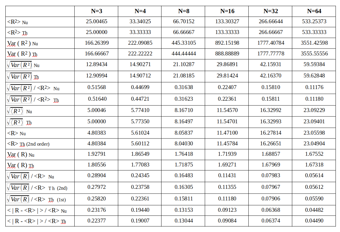
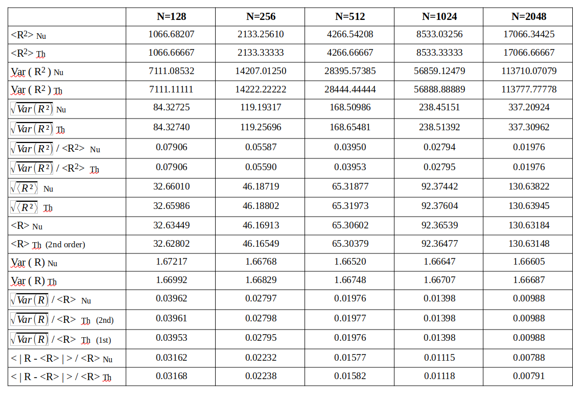
Afterwards I numerically evaluate the different statistical quantities named above – average radius, variance of the radius, standard deviation, ratios …. The statistics should be rather good with so many vectors. The following table provides a comparison between the numerically derived values and the theoretical approximations by our formulas.

A quantity evaluated numerically has a trailing Nu, a value derived via theoretical formulas a trailing Th in the first column of the tables. A line with a numerical value is followed by one or two lines with a theoretical prediction, sometimes including 2nd order corrections.

After my first post you will not be astonished that the R values get bigger than b with growing N. The graphics below shows the corresponding R-value distributions (very similar to the one explained in the first post):

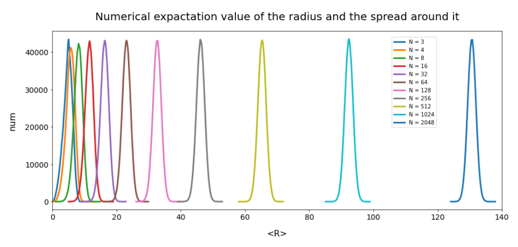
The data all in all prove that our vector creation based on a constant probability density per coordinate value does not at all fill our space in a homogeneous way for N > 4. Instead the generated vectors all approach a common length (radius) with growing N.

Interesting regions of the latent space we would miss

What regions would we miss in a high dimensional latent space with our simple vector distribution?

An important point, which one should keep in mind during the discussion, is that the results above do not indicate a homogeneously filled spherical shell. The results only tell us that we populate regions within such shells. So we have to think a bit about isotropy.

Another point is that defining the coordinates of a statistical vector in our case is similar to picking values N times from a mixing pot or trough containing small balls with imprinted values. The similarity becomes clear when we discretize our interval [-b, +b] into sub-intervals of equal length and assume a pot with small balls showing the mid-point of one particular interval on it.

Regions close to the origin

A first and obvious critical region is a spherical volume around the origin of the multi-dimensional space with a radius value small in comparison to

This follows from our derived characteristics of the radius distribution for the generated vectors. But it also follows from basic statistics: All N values for the coordinates must lie within an interval [0,r]. If you e.g. assume that r=1.0 and b=5, then the probability of creating such a point is (0.2)^N, which for all practical purposes is simply zero.

We can partially compensate for this deficit by creating many point distributions in successive nested cubes with systematically growing side lengths. If an Encoder had filled such a volume relatively densely we would thus have a chance to hit a part of the filled regions by some points of our distributions on growing multi-dimensional shells. However, we would still miss some other special regions.

Off-center regions with relatively big coordinate values only along a few axes

Now let us assume that an Encoder or an embedding part of a Neural Network has filled a region of our vector space which has the following characteristics:

1. The region is a kind of multi-dimensional ellipsoid with very limited extensions in most of its main axes.
2. Most coordinate values of points in our region are close to zero in an interval [-a, a] with a <(<) b. Only a few coordinate values (let us say for 10% of N >> 3 dimensions) are relatively big and lie in real number intervals [c, d] with |c| >(>) b. This places the points off-center.
3. The center of the filled region lies somewhere off the origin of the coordinate system and very close to or within a multidimensional volume spanned by only the few axes that are associated with larger coordinate values .

Now you may argue that a multi-dimensional spherical shell with the right radius should at least cut such an ellipsoid. True enough, but I warned you that the spherical shell we found might not be filled homogeneously!

If you need a 3D analogy: Think of a small 3D-ellipsoid elongated in x-direction, but with rather small diameters in both y- and z-direction. Place the center of this ellipsoid on the x-axis at a relatively high x-value, somewhat bigger than the ellipsoids x-extension (δy ≈ δy &approx 1, δ x = 4, x_center = 7, y_center=0, z_center = 0).
We saw already in our last post that our statistical vector distribution would not put many points into such an ellipsoid.

However, in a 256-dimensional space we would almost certainly miss such a region. The reason is that the statistics for our independently chosen coordinate values once again plays against us: Let us take b=10 (just to make calculations easier). Let us say that 220 coordinate values out of N=256 are within [-2,2] and for some coordinates in intervals [b1 >2, b2] with b2-b1 < 0.4*2b. Then the probability to create such a point is something like < 0.2²⁰⁰ * 0.4³⁶ ≈ = 0. Essentially zero again!

What we have just calculated reflects a fact we saw already for 3 dimensions: Narrow columns around one of the 3 coordinate axes receive only a few of our created points. The effect gets stronger with each added dimension – although our columns than have to be replaced by volume regions spanned by a few coordinate axes, only.

So our vector distribution is not homogeneous, but it is not even isotropic either. This makes it prone to miss major regions of the latent space.

Why are the named regions of interest?

I could and maybe should retract to experience with Autoencoders and word vector models here. I admit: I have no solid line of argumentation to follow here. Just some plausible speculations:

A deep neural network, e.g. a convolutional one, detects basic patterns and encodes them both in a defined number of internal filters or maps and vectors in some latent or embedding vector space, if we let the latter happen.

A latent vector tells a Decoder (of an Autoencoder) by the values of its components how to mix or superimpose a certain number of basic patterns. When encoding information into vectors the Encoder also must addresses typical characteristic fluctuations in patterns at the same time. Such fluctuations may naturally correspond to Gaussians around average values.

Think of images with human faces: There is a limited number of pixel correlation patterns that must be fulfilled for every face. Oval form of the face, two eyes with an average distance, 2 eye-brows, a nose in the middle, a mouth with or without visible teeth in some width, a certain complexion and color range of the skin, a certain hair-line. They all correspond to dominant patterns with some statistical variations in their characteristics. And they mark most of all bigger differences in real faces.

We have the length and the angles of latent vectors available to encode the differences between faces (and backgrounds).
It is natural to assume that fluctuations of peculiar patterns and also noise in less relevant features correspond to some Gaussian value variations. Gaussian distributions of many vector coordinates around a central zero value with vector length in a limited range already open up for many angles. This is ideal to encode different background variations.

It is also plausible to assume that the strength by which a certain pattern dominates the superposition can be encoded by the length of some vectors. Such vectors would point into certain directions as all faces have basic similarities. This would lead to vectors with end-points in coherent regions off-center. The variations in some dominant patterns nevertheless deserve a relatively broad region in the latent space – to get clear distinctions between classes of generated faces.

If all these speculations on encoding have a grain of truth than encoding certain objects with some dominant features could lead to coherent off-center regions with limited extensions and the center of which would lie within a volume spanned by a few of many coordinate axes. If this really were the case than our statistical vector distribution would be totally improper to hit such a region with at least a few vectors.

Conclusion

In this post we have numerically created a big bunch of statistical vectors which had the property that each of the coordinate values was defined independently and got a value from within a real number interval [-b, b] with uniform, constant probability. A numerical evaluation of the vector lengths, i.e. radius values, proved some theoretically derived formulas on the radius distribution. The vectors’ end points were indeed distributed within regions of a multi-dimensional spherical shell. And the shell got narrower with the number of available dimensions.

The resulting point distribution will neither fill regions around the origin uniformly nor isotropically.

Statistical arguments show that the points defined by our special vector distribution miss miss regions close to the origin. In addition the vectors will not hit coherent regions with limited extensions and with a center within volumes spanned by only a few of the many coordinate axes of the N-dimensional space. Unfortunately, such regions might be the ones which get filled by Encoders or embedding parts of some neural networks.

In the next post I will discuss why vector and point creation based on Gaussian probability distributions will not save us when we want to perform reasonable latent space surveys. Therefore, we must either enforce the Encoder networks to use certain regions of the latent vector spaces or we must in detail analyze the properties of the real multi-dimensional vector distribution created by an Encoder during its training.