We continue our article series on building a Python program for a MLP and training it to recognize handwritten digits on images of the MNIST dataset.
A simple Python program for an ANN to cover the MNIST dataset – XI – confusion matrix
A simple Python program for an ANN to cover the MNIST dataset – X – mini-batch-shuffling and some more tests
A simple Python program for an ANN to cover the MNIST dataset – IX – First Tests
A simple Python program for an ANN to cover the MNIST dataset – VIII – coding Error Backward Propagation
A simple Python program for an ANN to cover the MNIST dataset – VII – EBP related topics and obstacles
A simple Python program for an ANN to cover the MNIST dataset – VI – the math behind the „error back-propagation“
A simple Python program for an ANN to cover the MNIST dataset – V – coding the loss function
A simple Python program for an ANN to cover the MNIST dataset – IV – the concept of a cost or loss function
A simple Python program for an ANN to cover the MNIST dataset – III – forward propagation
A simple Python program for an ANN to cover the MNIST dataset – II – initial random weight values
A simple Python program for an ANN to cover the MNIST dataset – I – a starting point
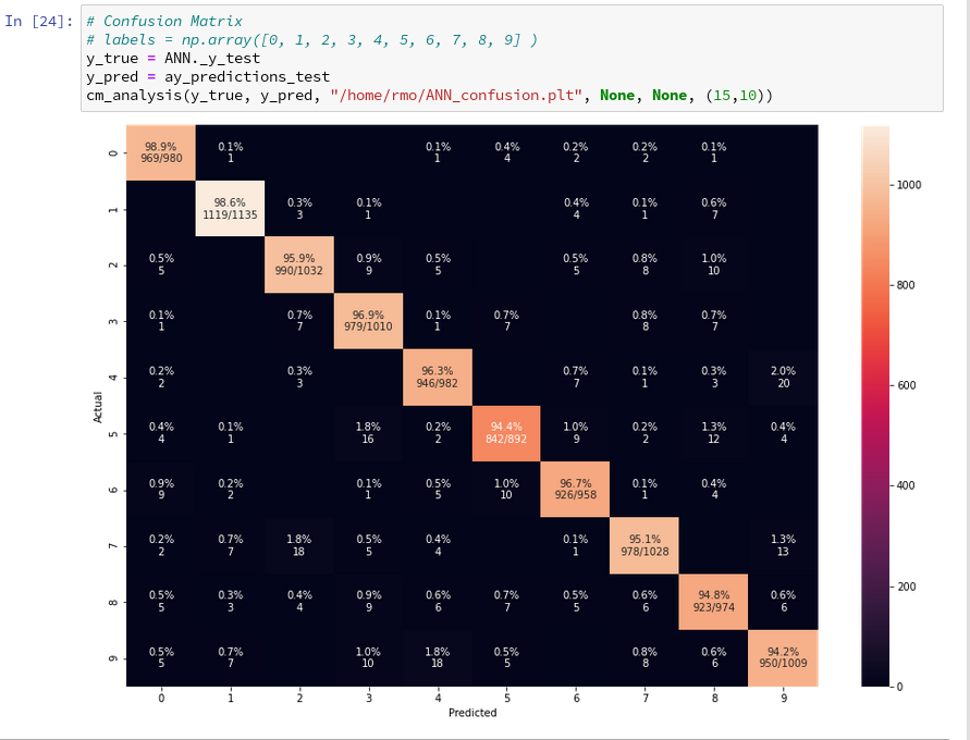
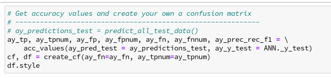
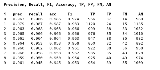
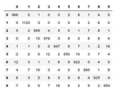
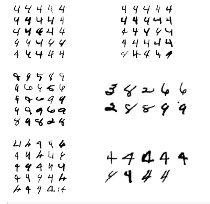
In the last article we used our prediction data to build a so called “confusion matrix” after training. With its help we got an overview about the “false negative” and “false positive” cases, i.e. cases of digit-images for which the algorithm made wrong predictions. We also displayed related critical MNIST images for the digit “4”.
In this article we first want to extend the ability of our class “ANN” such that we can measure the level of accuracy (more precisely: the recall) on the full test and the training data sets during training. We shall see that the resulting curves will trigger some new insights. We shall e.g. get an answer to the question at which epoch the accuracy on the test data set does no longer change, but the accuracy on the training set still improves. Meaning: We can find out after which epoch we spend CPU time on overfitting.
In addition we want to investigate the efficiency of our present approach a bit. So far we have used a relatively small learning rate of 0.0001 with a decrease rate of 0.000001. This gave us relatively smooth curves during convergence. However, it took us a lot of epochs and thus computational time to arrive at a cost
minimum. The question is:
Is a small learning rate really required? What happens if we use bigger initial learning rates? Can we reduce the number of epochs until learning converges?
Regarding the last point we should not forget that a bigger learning rate may help to move out of local minima on our way to the vicinity of a global minimum. Some of our experiments will indeed indicate that one may get stuck somewhere before moving deep into a minimum valley. However, our forthcoming experiments will also show that we have to take care about the weight initialization. And this in turn will lead us to a major deficit of our present code. Resolving it will help us with bigger learning rates, too.
Class interface changes
We introduce some new parameters, whose usage will become clear later on. They are briefly documented within the code. In addition we do no longer call the method _fit() automatically when we create a Python object instance of the class. This means the you have to call “_fit()” on your own in your Jupyter cells in the future.
To be able to use some additional features later on we first need some more import statements.
New import statements of the class MyANN
import numpy as np
import math
import sys
import time
import tensorflow
# from sklearn.datasets import fetch_mldata
from sklearn.datasets import fetch_openml
from sklearn.metrics import confusion_matrix
from sklearn.preprocessing import StandardScaler

from sklearn.cluster import KMeans
from sklearn.cluster import MiniBatchKMeans

from keras.datasets import mnist as kmnist
from scipy.special import expit
from matplotlib import pyplot as plt
from symbol import except_clause
from IPython.core.tests.simpleerr import sysexit
from math import floor
Extended My_ANN interface
We extend our interface substantially – although we shall not use every new parameter, yet. Most of the parameters are documented shortly; but to really understand what they control you have to look into some other changed parts of the class’s code, which we present later on. You can, however, safely ignore parameters on “clustering” and “PCA” in this article. We shall yet neither use the option to import MNIST X- and y-data (X_import, y_import) instead of loading them internally.
    def __init__(self,
                 my_data_set = "mnist",

                 X_import = None, # imported X dataset
                 y_import = None, # imported y dataset

                 num_test_records = 10000, # number of test data

                 # parameter for normalization of input data
                 b_normalize_X = False, # True: apply StandardScaler on X input data

                 # parameters for clustering of input data
                 b_perform_clustering = False,  # shall we cluster the X_data before learning?
                 my_clustering_method = "MiniBatchKMeans", # Choice between 2 methods: MiniBatchKMeans, KMeans
                 cl_n_clusters = 200,      # number of clusters (often "k" in literature)
                 cl_max_iter = 600,        # number of iterations for centroid movement
                 cl_n_init = 100,          # number of different initial centroid positions tried
                 cl_n_jobs = 4,            # number of CPU cores (jobs to start for investigating n_init variations
                 cl_batch_size = 500,      # batch size, only used for MiniBatchKMeans

                 #parameters for PCA of input data
                 b_
perform_pca = False,
                 num_pca_categories = 155,

                 # parameters for MLP structure
                 n_hidden_layers = 1,
                 ay_nodes_layers = [0, 100, 0], # array which should have as much elements as n_hidden + 2
                 n_nodes_layer_out = 10,  # expected number of nodes in output layer

                 my_activation_function = "sigmoid",
                 my_out_function        = "sigmoid",
                 my_loss_function       = "LogLoss",

                 n_size_mini_batch = 50,  # number of data elements in a mini-batch

                 n_epochs      = 1,
                 n_max_batches = -1,  # number of mini-batches to use during epochs - > 0 only for testing
                                      # a negative value uses all mini-batches

                 lambda2_reg = 0.1,     # factor for quadratic regularization term
                 lambda1_reg = 0.0,     # factor for linear regularization term

                 vect_mode = 'cols',

                 init_weight_meth_L0 = "sqrt_nodes",  # method to init weights => "sqrt_nodes", "const"
                 init_weight_meth_Ln = "sqrt_nodes",  # sqrt_nodes", "const"
                 init_weight_intervals = [(-0.5, 0.5), (-0.5, 0.5), (-0.5, 0.5)],   # size must fit number of hidden layers
                 init_weight_fact = 2.0,                # extends the interval


                 learn_rate = 0.001,          # the learning rate (often called epsilon in textbooks)
                 decrease_const = 0.00001,    # a factor for decreasing the learning rate with epochs
                 learn_rate_limit = 2.0e-05,  # a lower limit for the learn rate
                 adapt_with_acc = False,      # adapt learning rate with additional factor depending on rate of acc change
                 reduction_fact = 0.001,      # small reduction factor - should be around 0.001 because of an exponential reduction

                 mom_rate   = 0.0005,         # a factor for momentum learning

                 b_shuffle_batches = True,    # True: we mix the data for mini-batches in the X-train set at the start of each epoch

                 b_predictions_train = False, # True: At the end of periodic epochs the code performs predictions on the train data set
                 b_predictions_test  = False, # True: At the end of periodic epochs the code performs predictions on the test data set
                 prediction_test_period  = 1, # Period of epochs for which we perform predictions
                 prediction_train_period = 1, # Period of epochs for which we perform predictions

                 print_period = 20,         # number of epochs for which to print the costs and the averaged error

                 figs_x1=12.0, figs_x2=8.0,
                 legend_loc='upper right',

                 b_print_test_data = True

                 ):
        '''
        Initialization of MyANN
        Input:
            data_set: type of dataset; so far only the "mnist", "mnist_784" datsets are known
                      We use this information to prepare the input data and learn about the feature dimension.
                      This info is used in preparing the size of the input layer.

            X_import: external X dataset to import
            y_import: external y dataset to import - must fit in dimension to X_import

            num_test_records: number of test data

            b_normalize_X: True => Invoke the StandardScaler of
Scikit-Learn
                                   to center and normalize the input data X

            Preprocessing of input data treatment before learning
            ------------------------------------
            Clustering
            -----------
            b_perform_clustering   # True => Cluster the X_data before learning?
            my_clustering_method   # string: 2 methods: MiniBatchKMeans, KMeans
            cl_n_clusters = 200       # number of clusters (often "k" in literature)
            cl_max_iter = 600      # number of iterations for centroid movement
            cl_n_init = 100        # number of different initial centroid positions tried
            cl_n_jobs = 4,         # number of CPU cores => jobs - only used for "KMeans"
            cl_batch_size = 500    # batch size used for "MiniBatchKMeans"

            PCA
            -----
            b_perform_pca: True => perform a pca analysis
            num_pca_categories: 155 - choose a reasonable number

            n_hidden_layers = number of hidden layers => between input layer 0 and output layer n

            ay_nodes_layers = [0, 100, 0 ] : We set the number of nodes in input layer_0 and the output_layer to zero
                              Will be set to real number afterwards by infos from the input dataset.
                              All other numbers are used for the node numbers of the hidden layers.
            n_nodes_out_layer = expected number of nodes in the output layer (is checked);
                                this number corresponds to the number of categories NC = number of labels to be distinguished

            my_activation_function : name of the activation function to use
            my_out_function : name of the "activation" function of the last layer which produces the output values
            my_loss_function : name of the "cost" or "loss" function used for optimization

            n_size_mini_batch : Number of elements/samples in a mini-batch of training data
                                The number of mini-batches will be calculated from this

            n_epochs : number of epochs to calculate during training
            n_max_batches : > 0: maximum of mini-batches to use during training
                            < 0: use all mini-batches

            lambda_reg2:    The factor for the quadartic regularization term
            lambda_reg1:    The factor for the linear regularization term

            vect_mode: Are 1-dim data arrays (vctors) ordered by columns or rows ?

            init_weight_meth_L0: Method to calculate the initial weights at layer L0: "sqrt_nodes" => sqrt(number of nodes) /  "const" => interval borders
            init_weight_meth_Ln: Method to calculate the initial weights at hidden layers
            init_weight_intervals: list of tuples with interval limits [(-0.5, 0.5), (-0.5, 0.5), (-0.5, 0.5)],
                                   size must fit number of hidden layers
            init_weight_fact:  interval limits get scald by this factor, e.g. 2* (0,5, 0.5)

            learn rate :     Learning rate - definies by how much we correct weights in the indicated direction of the gradient on the cost hyperplane.
            decrease_const:  Controls a systematic decrease of the learning rate with epoch number
            learn_rate_limit = 2.0e-05,  # a lowee limit for the learning rate

            adapt_with_acc:  True => adapt learning rate with additional factor depending on rate of acc change
            reduction_fact:  around 0.001  => almost exponential reduction during the first 500 epochs

            mom_const:       Momentum rate. Controls a mixture of the last with the present weight
corrections (momentum learning)

            b_shuffle_batches: True => vary composition of mini-batches with each epoch

            # The next two parameters enable the measurement of accuracy and total cost function
            # by making predictions on the train and test datasets
            b_predictions_train: True => perform a prediction run on the full training data set => get accuracy
            b_predictions_test:  True => perform a prediction run on the full test data set => get accuracy
            prediction_test_period: period of epochs for which to perform predictions
            prediction_train_period: period of epochs for which to perform predictions

            print_period:    number of periods between printing out some intermediate data
                             on costs and the averaged error of the last mini-batch


            figs_x1=12.0, figs_x2=8.0 : Standard sizing of plots ,
            legend_loc='upper right': Position of legends in the plots

            b_print_test_data: Boolean variable to control the print out of some tests data

         '''

        # Array (Python list) of known input data sets
        self._input_data_sets = ["mnist", "mnist_784", "mnist_keras", "imported"]
        self._my_data_set = my_data_set

        # X_import, y_import, X, y, X_train, y_train, X_test, y_test
            # will be set by method handle_input_data()
            # X: Input array (2D) - at present status of MNIST image data, only.
            # y: result (=classification data) [digits represent categories in the case of Mnist]
        self._X_import = X_import
        self._y_import = y_import

        # number of test data
        self._num_test_records = num_test_records

        self._X       = None
        self._y       = None
        self._X_train = None
        self._y_train = None
        self._X_test  = None
        self._y_test  = None

        # perform a normalization of the input data
        self._b_normalize_X = b_normalize_X

        # relevant dimensions
        # from input data information;  will be set in handle_input_data()
        self._dim_X        = 0  # total num of records in the X,y input sets
        self._dim_sets     = 0  # num of records in the TRAINING sets X_train, y_train
        self._dim_features = 0
        self._n_labels     = 0   # number of unique labels - will be extracted from y-data

        # Img sizes
        self._dim_img      = 0 # should be sqrt(dim_features) - we assume square like images
        self._img_h        = 0
        self._img_w        = 0

        # Preprocessing of input data
        # ---------------------------
        self._b_perform_clustering = b_perform_clustering
        self._my_clustering_method = my_clustering_method # for the related dictionary see below
        self._kmeans        = None   # pointer to object used for clustering
        self._cl_n_clusters = cl_n_clusters       # number of clusters (often "k" in literature)
        self._cl_max_iter   = cl_max_iter      # number of iterations for centroid movement
        self._cl_n_init     = cl_n_init        # number of different initial centroid positions tried
        self._cl_batch_size = cl_batch_size    # batch size used for MiniBatchKMeans
        self._cl_n_jobs     = cl_n_jobs        # number of parallel jobs (on CPU-cores) - only used for KMeans

        # Layers
        # ------
        # number of hidden layers
        self._n_hidden_layers = n_hidden_layers
        # Number of total layers
        self._n_total_layers = 2 + self._n_hidden_layers
        # Nodes for hidden layers

self._ay_nodes_layers = np.array(ay_nodes_layers)
        # Number of nodes in output layer - will be checked against information from target arrays
        self._n_nodes_layer_out = n_nodes_layer_out

        # Weights
        # --------
        # empty List for all weight-matrices for all layer-connections
        # Numbering :
        # w[0] contains the weight matrix which connects layer 0 (input layer ) to hidden layer 1
        # w[1] contains the weight matrix which connects layer 1 (input layer ) to (hidden?) layer 2
        self._li_w = []

        # Arrays for encoded output labels - will be set in _encode_all_mnist_labels()
        # -------------------------------
        self._ay_onehot = None
        self._ay_oneval = None

        # Known Randomizer methods ( 0: np.random.randint, 1: np.random.uniform )
        # ------------------
        self.__ay_known_randomizers = [0, 1]

        # Types of activation functions and output functions
        # ------------------
        self.__ay_activation_functions = ["sigmoid"] # later also relu
        self.__ay_output_functions     = ["sigmoid"] # later also softmax

        # Types of cost functions
        # ------------------
        self.__ay_loss_functions = ["LogLoss", "MSE" ] # later also other types of cost/loss functions


        # dictionaries for indirect function calls
        self.__d_activation_funcs = {
            'sigmoid': self._sigmoid,
            'relu':    self._relu
            }
        self.__d_output_funcs = {
            'sigmoid': self._sigmoid,
            'softmax': self._softmax
            }
        self.__d_loss_funcs = {
            'LogLoss': self._loss_LogLoss,
            'MSE': self._loss_MSE
            }
        # Derivative functions
        self.__d_D_activation_funcs = {
            'sigmoid': self._D_sigmoid,
            'relu':    self._D_relu
            }
        self.__d_D_output_funcs = {
            'sigmoid': self._D_sigmoid,
            'softmax': self._D_softmax
            }
        self.__d_D_loss_funcs = {
            'LogLoss': self._D_loss_LogLoss,
            'MSE': self._D_loss_MSE
            }
        self.__d_clustering_functions = {
            'MiniBatchKMeans': self._Mini_Batch_KMeans,
            'KMeans': self._KMeans
            }

        # The following variables will later be set by _check_and set_activation_and_out_functions()
        self._my_act_func  = my_activation_function
        self._my_out_func  = my_out_function
        self._my_loss_func = my_loss_function
        self._act_func      = None
        self._out_func      = None
        self._loss_func     = None
        self._cluster_func  = None

        # number of data samples in a mini-batch
        self._n_size_mini_batch = n_size_mini_batch
        self._n_mini_batches = None  # will be determined by _get_number_of_mini_batches()

        # maximum number of epochs - we set this number to an assumed maximum
        # - as we shall build a backup and reload functionality for training, this should not be a major problem
        self._n_epochs = n_epochs

        # maximum number of batches to handle ( if < 0 => all!)
        self._n_max_batches = n_max_batches
        # actual number of batches
        self._n_batches = None

        # regularization parameters
        self._lambda2_reg = lambda2_reg
        self._lambda1_reg = lambda1_reg

        # parameters to control the initialization of the weights (see _create_WM_Input(), create_WM_Hidden())
        self._init_weight_meth_L0 = init_weight_meth_L0
        self._init_weight_meth_Ln = init_weight_meth_Ln
        self._init_weight_
intervals = init_weight_intervals # list of lists with interval borders
        self._init_weight_fact = init_weight_fact           # extends weight intervals


        # parameters for adaption of the learning rate
        self._learn_rate = learn_rate
        self._decrease_const = decrease_const
        self._learn_rate_limit = learn_rate_limit
        self._adapt_with_acc  = adapt_with_acc
        self._reduction_fact  = reduction_fact
        #
        # parameters for momentum learning
        self._mom_rate   = mom_rate
        self._li_mom = [None] *  self._n_total_layers

        # shuffle data in X_train?
        self._b_shuffle_batches = b_shuffle_batches

        # perform predictions on train and test data set and related analysis
        self._b_predictions_train = b_predictions_train
        self._b_predictions_test  = b_predictions_test
        self._prediction_test_period  = prediction_test_period
        self._prediction_train_period = prediction_train_period

        # epoch period for printing
        self._print_period = print_period

        # book-keeping for epochs and mini-batches
        # -------------------------------
        # range for epochs - will be set by _prepare-epochs_and_batches()
        self._rg_idx_epochs = None
        # range for mini-batches
        self._rg_idx_batches = None
        # dimension of the numpy arrays for book-keeping - will be set in _prepare_epochs_and_batches()
        self._shape_epochs_batches = None    # (n_epochs, n_batches, 1)

        # training evolution:
        # +++++++++++++++++++
        # List for error values at outermost layer for minibatches and epochs during training
        # we use a numpy array here because we can redimension it
        self._ay_theta = None
        # List for cost values of mini-batches during training - The list will later be split into sections for epochs
        self._ay_costs = None
        #
        # List for test accuracy values and error values at epoch periods
        self._ay_period_test_epoch = None # x-axis for plots of the following 2 quantities
        self._ay_acc_test_epoch = None
        self._ay_err_test_epoch = None
        # List for train accuracy values and error values at epoch periods
        self._ay_period_train_epoch = None # x-axis for plots of the following 2 quantities
        self._ay_acc_train_epoch = None
        self._ay_err_train_epoch = None

        # Data elements for back propagation
        # ----------------------------------

        # 2-dim array of partial derivatives of the elements of an additive cost function
        # The derivative is taken with respect to the output results a_j = ay_ANN_out[j]
        # The array dimensions account for nodes and sampls of a mini_batch. The array will be set in function
        # self._initiate_bw_propagation()
        self._ay_delta_out_batch = None


        # parameter to allow printing of some test data
        self._b_print_test_data = b_print_test_data

        # Plot handling
        # --------------
        # Alternatives to resize plots
        # 1: just resize figure  2: resize plus create subplots() [figure + axes]
        self._plot_resize_alternative = 1
        # Plot-sizing
        self._figs_x1 = figs_x1
        self._figs_x2 = figs_x2
        self._fig = None
        self._ax  = None
        # alternative 2 does resizing and (!) subplots()
        self.initiate_and_resize_plot(self._plot_resize_alternative)


        # ***********
        # operations
        # ***********

        # check and handle input data
        self._handle_input_data()
        # set the ANN structure
        self._set_ANN_structure()


   # Prepare epoch and batch-handling - sets ranges, limits num of mini-batches and initializes book-keeping arrays
        self._rg_idx_epochs, self._rg_idx_batches = self._prepare_epochs_and_batches()
Code modifications to create precise accuracy information on the full test and training sets during training
You certainly noticed the following set of control parameters in the class’s new interface:
- b_predictions_train = False, # True: At the end of periodic epochs the code performs predictions on the train data set
- b_predictions_test = False, # True: At the end of periodic epochs the code performs predictions on the test data set
- prediction_test_period = 1, # Period of epochs for which we perform predictions
- prediction_train_period = 1, # Period of epochs for which we perform predictions
These parameters control whether we perform predictions during training for the full test dataset and/or the full training dataset – and if so, at which epoch period. Actually, during all of the following experiments we shall evaluate the accuracy data after each single period.
We need an array to gather accuracy information. We therefore modify the method “_prepare_epochs_and_batches()”, where we fill some additional Numpy arrays with initialization values. Thus we avoid a costly “append()” later on; we just overwrite the array entries successively. This overwriting happens in our method _fit(); see below.
Changes to function “_prepare_epochs_and_batches()”:
    ''' -- Main Method to prepare epochs, batches and book-keeping arrays -- '''
    def _prepare_epochs_and_batches(self, b_print = True):
        # range of epochs
        ay_idx_epochs  = range(0, self._n_epochs)

        # set number of mini-batches and array with indices of input data sets belonging to a batch
        self._set_mini_batches()

        # limit the number of mini-batches
        self._n_batches = min(self._n_max_batches, self._n_mini_batches)
        ay_idx_batches = range(0, self._n_batches)
        if (b_print):
            if  self._n_batches < self._n_mini_batches :
                print("\nWARNING: The number of batches has been limited from " +
                      str(self._n_mini_batches) + " to " + str(self._n_max_batches) )

        # Set the book-keeping arrays
        self._shape_epochs_batches = (self._n_epochs, self._n_batches)
        self._ay_theta = -1 * np.ones(self._shape_epochs_batches) # float64 numbers as default
        self._ay_costs = -1 * np.ones(self._shape_epochs_batches) # float64 numbers as default

        shape_test_epochs  = ( floor(self._n_epochs / self._prediction_test_period), )
        shape_train_epochs = ( floor(self._n_epochs / self._prediction_train_period), )
        self._ay_period_test_epoch  = -1 * np.ones(shape_test_epochs) # float64 numbers as default
        self._ay_acc_test_epoch     = -1 * np.ones(shape_test_epochs) # float64 numbers as default
        self._ay_err_test_epoch     = -1 * np.ones(shape_test_epochs) # float64 numbers as default
        self._ay_period_train_epoch = -1 * np.ones(shape_train_epochs) # float64 numbers as default
        self._ay_acc_train_epoch    = -1 * np.ones(shape_train_epochs) # float64 numbers as default
        self._ay_err_train_epoch    = -1 * np.ones(shape_train_epochs) # float64 numbers as default

        return ay_idx_epochs, ay_idx_batches
#
We then create two new methods to calculate accuracy values by predicting results on all records of both the training dataset and the test dataset. The attentive reader certainly recognizes the methods’ structure from a previous article where we used
similar code in a Jupyter cell:
New functions “_predict_all_test_data()” and “_predict_all_train_data()”:
    ''' Method to predict values for the full set of test data '''
    def _predict_all_test_data(self):
        size_set = self._X_test.shape[0]

        li_Z_in_layer_test  = [None] * self._n_total_layers
        li_Z_in_layer_test[0] = self._X_test

        # Transpose input data matrix
        ay_Z_in_0T       = li_Z_in_layer_test[0].T
        li_Z_in_layer_test[0] = ay_Z_in_0T
        li_A_out_layer_test  = [None] * self._n_total_layers

        # prediction by forward propagation of the whole test set
        self._fw_propagation(li_Z_in = li_Z_in_layer_test, li_A_out = li_A_out_layer_test, b_print = False)
        ay_predictions_test = np.argmax(li_A_out_layer_test[self._n_total_layers-1], axis=0)

        # accuracy
        ay_errors_test = self._y_test - ay_predictions_test
        acc_test = (np.sum(ay_errors_test == 0)) / size_set
        # print ("total acc for test data = ", acc)
        # return acc, ay_predictions_test
        return acc_test
#
    ''' Method to predict values for the full set of training data '''
    def _predict_all_train_data(self):
        size_set = self._X_train.shape[0]

        li_Z_in_layer_train  = [None] * self._n_total_layers
        li_Z_in_layer_train[0] = self._X_train
        # Transpose
        ay_Z_in_0T       = li_Z_in_layer_train[0].T
        li_Z_in_layer_train[0] = ay_Z_in_0T
        li_A_out_layer_train  = [None] * self._n_total_layers

        self._fw_propagation(li_Z_in = li_Z_in_layer_train, li_A_out = li_A_out_layer_train, b_print = False)
        ay_predictions_train = np.argmax(li_A_out_layer_train[self._n_total_layers-1], axis=0)
        ay_errors_train = self._y_train - ay_predictions_train
        acc_train = (np.sum(ay_errors_train == 0)) / size_set
        #print ("total acc for train data = ", acc)

        return acc_train
#
Eventually, we modify our method “_fit()” with a series of statements on the level of the epoch loop. You may ignore most of the statements for learning rate adaption; we only use the “simple” adaption methods. The really important changes are those regarding predictions.
Modifications of function “_fit()”:
    ''' -- Method to perform training in epochs for defined mini-batches -- '''
    def _fit(self, b_print = False, b_measure_epoch_time = True, b_measure_batch_time = False):
        '''
        Parameters:
            b_print:                 Do we print intermediate results of the training at all?
            b_print_period:          For which period of epochs do we print?
            b_measure_epoch_time:    Measure CPU-Time for an epoch
            b_measure_batch_time:    Measure CPU-Time for a batch
        '''
        rg_idx_epochs  = self._rg_idx_epochs
        rg_idx_batches = self._rg_idx_batches
        if (b_print):
            print("\nnumber of epochs = " + str(len(rg_idx_epochs)))
            print("max number of batches = " + str(len(rg_idx_batches)))

        # Some intial parameters
        acc_old = 0.0000001
        acc_test = 0.001
        orig_rate = self._learn_rate
        adapt_fact = 1.0
        n_predict_test  = 0
        n_predict_train = 0

        # loop over epochs
        # ****************
        start_train = time.perf_counter()
        for idxe in rg_idx_epochs:
            if b_print and (idxe % self._print_period == 0):
                if b_measure_epoch_time:

          start_0_e = time.perf_counter()
                print("\n ---------")
                print("Starting epoch " + str(idxe+1))

            # simple adaption of the learning rate
            # ~~~~~~~~~~~~~~~~~~~~~~~~~~~~~~~~~~~~
            orig_rate /= (1.0 + self._decrease_const * idxe)
            self._learn_rate /= (1.0 + self._decrease_const * idxe)
            if self._learn_rate < self._learn_rate_limit:
                self._learn_rate = self._learn_rate_limit

            # adapt wit acc. - not working well, yet
            #~~~~~~~~~~~~~~~~~~~~~~~~~~~~~~~~~~~~~~~
            acc_change_rate = math.fabs((acc_test - acc_old) / acc_old)
            if b_print and (idxe % self._print_period == 0):
                print("acc_chg_rate = ", acc_change_rate)
            ratio = self._learn_rate / orig_rate
            if ratio > 0.33 and acc_change_rate < 1/3 and self._adapt_with_acc:
                if acc_change_rate < 0.001:
                    acc_change_rate = 0.001
                #adapt_fact = 2.0 * acc_change_rate / (1.0 - acc_change_rate)
                adapt_fact = 1.0 - 0.001 * (1.0 - acc_change_rate / (1.0 - acc_change_rate))
                if b_print and (idxe % self._print_period == 0):
                    print("adapt_fact = ", adapt_fact)
                self._learn_rate *= adapt_fact
            acc_old = acc_test # for adaption of learning rate

            # shuffle indices for a variation of the mini-batches with each epoch
            # ******************************************************************
            if self._b_shuffle_batches:
                shuffled_index = np.random.permutation(self._dim_sets)
                self._X_train, self._y_train, self._ay_onehot = self._X_train[shuffled_index], self._y_train[shuffled_index], self._ay_onehot[:, shuffled_index]
            #
            # loop over mini-batches
            # **********************
            for idxb in rg_idx_batches:
                if b_measure_batch_time:
                    start_0_b = time.perf_counter()
                # deal with a mini-batch
                self._handle_mini_batch(num_batch = idxb, num_epoch=idxe, b_print_y_vals = False, b_print = False)
                if b_measure_batch_time:
                    end_0_b = time.perf_counter()
                    print('Time_CPU for batch ' + str(idxb+1), end_0_b - start_0_b)

            #
            # predictions
            # ***********
            # Control and perform predictions on the full test data set
            if self._b_predictions_test and idxe % self._prediction_test_period == 0:
                self._ay_period_test_epoch[n_predict_test] = idxe
                acc_test = self._predict_all_test_data()
                self._ay_acc_test_epoch[n_predict_test] = acc_test
                n_predict_test += 1
            # Control and perform predictions on the full training training data set
            if self._b_predictions_train and idxe % self._prediction_train_period == 0:
                self._ay_period_train_epoch[n_predict_train] = idxe
                acc_train = self._predict_all_train_data()
                self._ay_acc_train_epoch[n_predict_train] = acc_train
                n_predict_train += 1
            #
            # printing some evolution and epoch information
            if b_print and (idxe % self._print_period == 0):
                if b_measure_epoch_time:
                    end_0_e = time.perf_counter()
                    print('Time_CPU for epoch' + str(idxe+1), end_0_e - start_0_e)
                print("learning rate = ", self._learn_rate)
                print("orig learn rate = ", orig_rate)
                print("\ntotal costs of last mini_batch = ", self._ay_costs[idxe, idxb])
                print("avg total error of
last mini_batch = ", self._ay_theta[idxe, idxb])
                # print presently reached accuracy values on the test and training sets
                print("presently reached train accuracy =<div style="width: 95%; overflow: auto; height: 400px;">
<pre style="width: 1000px;">
 ", acc_train)
                print("presently reached test accuracy = ", acc_test)

        # print out required secs for training
        # **************************************
        end_train = time.perf_counter()
        print('\n\n ------')
        print('Total training Time_CPU: ', end_train - start_train)
        print("\nStopping program regularily")

        return None
#
The method we apply in the above code to reduce the learning rate with every epoch is by the way called “power scheduling“. The book of Aurelien Geron [“Hands on Machine learning ….”, 2019, 2nd edition, O’Reilly], quoted already in previous articles, lists a bunch of other methods, e.g. “exponential scheduling”, where we multiply the learning rate with a constant factor < 1 at every epoch.
A further change of code happens in the functions _create_WM_input() and _ceate_WM_hidden” to initiate weight values.
Modifications of functions _create_WM_input() and _create_WM_hidden”:
Addendum 25.03.2020: Changed _create_WM_hidden() because of errors in the code
    '''-- Method to create the weight matrix between L0/L1 --'''
    def _create_WM_Input(self):
        '''
        Method to create the input layer
        The dimension will be taken from the structure of the input data
        We need to fill self._w[0] with a matrix for conections of all nodes in L0 with all nodes in L1
        We fill the matrix with random numbers between [-1, 1]
        '''
        # the num_nodes of layer 0 should already include the bias node
        num_nodes_layer_0 = self._ay_nodes_layers[0]
        num_nodes_with_bias_layer_0 = num_nodes_layer_0 + 1
        num_nodes_layer_1 = self._ay_nodes_layers[1]

        # Set interval borders for randomizer
        if self._init_weight_meth_L0 == "sqrt_nodes":  # sqrtr(nodes) - rule of Prof. J. Frochte
            rand_high = self._init_weight_fact / math.sqrt(float(num_nodes_layer_0))
            rand_low = - rand_high
        else:
            rand_low  = self._init_weight_intervals[0][0]
            rand_high = self._init_weight_intervals[0][1]
        print("\nL0: weight range [" + str(rand_low) + ", " + str(rand_high) + "]" )

        # fill the weight matrix at layer L0 with random values
        randomizer = 1 # method np.random.uniform
        rand_size = num_nodes_layer_1 * (num_nodes_with_bias_layer_0)
        w0 = self._create_vector_with_random_values(rand_low, rand_high, rand_size, randomizer)
        w0 = w0.reshape(num_nodes_layer_1, num_nodes_with_bias_layer_0)

        # put the weight matrix into array of matrices
        self._li_w.append(w0)
        print("\nShape of weight matrix between layers 0 and 1 " + str(self._li_w[0].shape))

#
    '''-- Method to create the weight-matrices for hidden layers--'''
    def _create_WM_Hidden(self):
        '''
        Method to create the weights of the hidden layers, i.e. between [L1, L2] and so on ... [L_n, L_out]
        We fill the matrix with random numbers between [-1, 1]
        '''

        # The "+1" is required due to range properties !
        rg_hidden_layers = range(1, self._n_hidden_layers + 1, 1)

        # Check parameter input fro weight intervals
        if self._init_weight_meth_Ln == "const":
            if len(self._init_
weight_intervals) != (self._n_hidden_layers + 1):
                print("\nError: we shall initialize weights with values from intervals, but wrong number of intervals provided!")
                sys.exit()

        for i in rg_hidden_layers:
            print ("\nCreating weight matrix for layer " + str(i) + " to layer " + str(i+1) )

            num_nodes_layer = self._ay_nodes_layers[i]
            num_nodes_with_bias_layer = num_nodes_layer + 1

            # Set interval borders for randomizer
            if self._init_weight_meth_Ln == "sqrt_nodes":  # sqrtr(nodes) - rule of Prof. J. Frochte
                rand_high = self._init_weight_fact / math.sqrt(float(num_nodes_layer))
                rand_low = - rand_high
            else:
                rand_low  = self._init_weight_intervals[i][0]
                rand_high = self._init_weight_intervals[i][1]
            print("L" + str(i) + ": weight range [" + str(rand_low) + ", " + str(rand_high) + "]" )

            # the number of the next layer is taken without the bias node!
            num_nodes_layer_next = self._ay_nodes_layers[i+1]

            # ill the weight matrices at the hidden layer with random values
            rand_size = num_nodes_layer_next * num_nodes_with_bias_layer
            randomizer = 1 # np.random.uniform
            w_i_next = self._create_vector_with_random_values(rand_low, rand_high, rand_size, randomizer)
            w_i_next = w_i_next.reshape(num_nodes_layer_next, num_nodes_with_bias_layer)

            # put the weight matrix into our array of matrices
            self._li_w.append(w_i_next)
            print("Shape of weight matrix between layers " + str(i) + " and " + str(i+1) + " = " + str(self._li_w[i].shape))
#
As you see, we distinguish between different cases depending on the parameters “init_weight_meth_L0” and “init_weight_meth_Ln”. There, obviously, happens a choice regarding the borders of the intervals from which we randomly pick our initial weight values. In case of the method “sqrt_nodes” the interval borders are determined by the number of nodes of the neighboring layer. Otherwise we can read the interval borders from the parameter list “init_weight_intervals”. You will better understand these options later on.
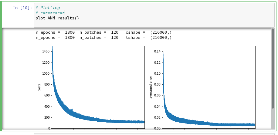
Plotting accuracys
We use a very simple code in a Jupyter cell to get a plot for the accuracy values on the training and the test datasets. The orange line will show the accuracy reached at each epoch for the training dataset when we apply the weights evaluated given at the epoch. The blue line shows the accuracy reached for the test dataset. In the text below we shall use the following abbreviations:
acc_train = accuracy reached for the X_train dataset of MNIST
acc_test = accuracy reached for the X_test dataset of MNIST
Code for plotting
y_min=0.75
y_max=1.0
plt.xlim(0,1800)
plt.ylim(y_min, y_max)

xplot=ANN._ay_period_test_epoch
yplot=ANN._ay_acc_test_epoch
plt.plot(xplot,yplot)

xplot=ANN._ay_period_train_epoch
yplot=ANN._ay_acc_train_epoch
plt.plot(xplot,yplot)
plt.show()
Experiment 1: Accuracy plot for a Reference Run
The next test run will be used as a reference run for comparisons later on. It shows where we stand right now.
Test 1:
Parameters: learn_rate = 0.0001, decrease_rate = 0.000001, mom_rate = 0.00005, n_size_mini_batch = 500, Lambda2 = 0.2, n_epochs = 1800, initial weights for all layers in [-0.5, +0.5]:
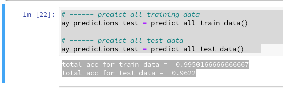
Results: acc_train: 0.996 , acc_test: 0.961, convergence after ca. 1150 epochs
Note that we use a very small learn_rate, but an even smaller decrease rate. The
evolution of the accuracy values looks like follows:
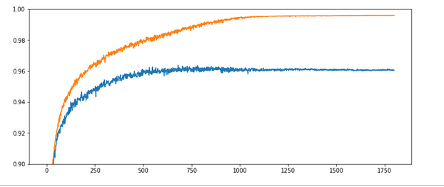
The x-axis measures the number of epochs during training. The y-axis the degree of accuracy – given as a fraction; multiply by 100 to get percentage values. By the way, applying the reached weight set on the full training and test datasets in each epoch cost us at least 20% rise in CPU time (45 minutes).
What does our new way of representing the “learning” of our MLP by the evolution of the accuracy levels tell us?
Noise: There is substantial noise visible along the lines. If you go back to previous articles you may detect the same type of noise in the plots of the evolution of the cost function. Obviously, our mini-batches and the constant change of their composition with each epoch lead to wiggles around the visible trends.
Tendencies: Note that there is a tendency of linear rise of the accuracy acc_train between periods 350 and 900. And, actually, the accuracy even decreases a bit around epoch 1550. This is a warning that the very last epoch of a run may not reveal the optimal solution.
Overfitting and a typical related splitting of the evolution of the two accuracys: One clearly sees that after a certain epoch (here: around epoch 300) the accuracy on the training dataset deviates systematically from the accuracy on the test dataset. In the end the gap is bigger than 3.5 percent. And in our case the accuracy on the test dataset reaches its final level of 0.96 significantly earlier – at around epoch 750 – and remains there, while the accuracy on the training set still rises up to epoch 1000.
However, I would like to add a warning:
Warning: Later on we shall see that there are cases for which both curves turn into a convergence at almost the same epoch. So, yes, there almost always occurs some overfitting during training of a MLP. However, we cannot set up a rule which says that convergence of the accuracy on the test dataset always occurs much earlier than for the training set. You always have to watch the evolution of both during your training experiments!
Experiment 2: Increasing the learning rate – better efficiency?
Let us now be brave and increase the learning rate by a factor of 10:
Test 2:
Parameters: learn_rate = 0.001, decrease_rate = 0.000001, mom_rate = 0.00005, n_size_mini_batch = 500, Lambda2 = 0.2, n_epochs = 1800, initial weights for all layers in [-0.5, +0.5]:
Results: acc_train: 0.971 , acc_test: 0.959, no convergence after ca. 1800 epochs, yet
Ooops! Our algorithm ran into real difficulties! We seem to hop in and out of a minimum area until epoch 400 and despite a following systematic linear improvementthere is no sign of a real convergence – yet!
The learning rate seems to big to lead to a consistent quick path into a minimum of all mini-batches! This may have to do with the size of the mini-batches, too – see below. The increase of the learning rate did not do us any good.
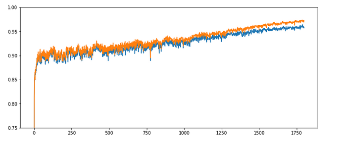
Experiment 3: Increased learning rate – but a higher decrease rate, too
As the larger learning rate seems to be a problem after period 50, we may think of a faster reduction of the learning rate.
Test 3:
Parameters: learn_rate = 0.001, decrease_rate = 0.00001, mom_rate = 0.00005, n_
size_mini_batch = 500, Lambda2 = 0.2, n_epochs = 2000, initial weights for all layers in [-0.5, +0.5]:
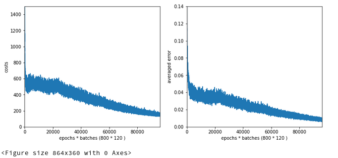
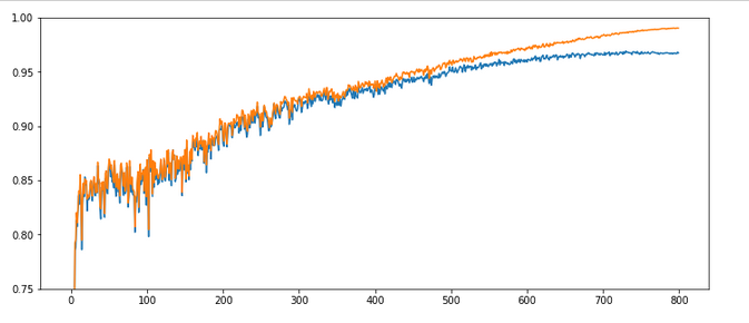
Results: acc_train: 0.9909, acc_test: 0.9646, convergence after ca. 800 epochs
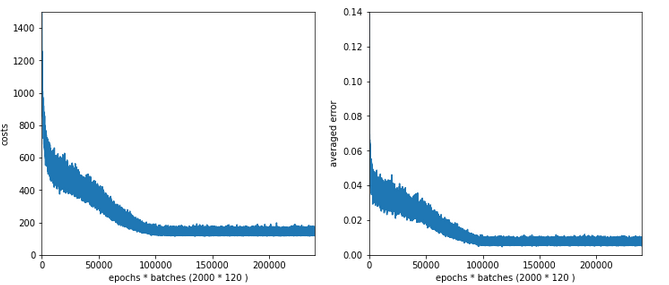
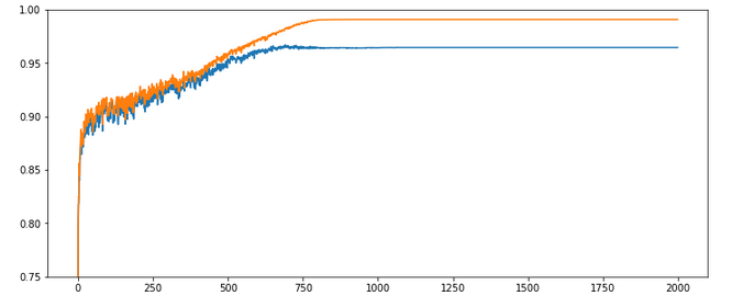
The evolution looks strange, too, but better than experiment 2! We see a real convergence again after some rather linear development! As a lesson learned I would say: Yes we can work with an initially bigger learning rate – but we need a stronger decrease of it, too, to really run into a global minimum eventually.
Experiment 4: Increased learning rate, higher decrease rate and smaller initial weights
Maybe the weight initialization has some impact? According to a rule published by Prof. Frochte in his book “Maschinelles Lernen” [2019, 2. Auflage, Carl Hanser Verlag] I limited the initial random weight values to a range between [-1.0/sqrt(784), +1.0/sqrt(784)] – instead of [-0.5, 0.5] for all layers.
Test 4:
Parameters: learn_rate = 0.001, decrease_rate = 0.00001, mom_rate = 0.00005, n_size_mini_batch = 500, Lambda2 = 0.2, n_epochs = 2000, initial weights for all layers within [-0.36 0.36]:
Results: acc_train: 0.987 , acc_test: 0.967, convergence after ca. 900 epochs
The interesting part in this case happens below and at epoch 200: There we see a clear indication that something has “trapped” us for a while before we could descend into some minimum with the typical split of the accuracy for the training set and the accuracy for the test set. Remember that smaller initial weights also mean an initially smaller contribution of the regularization term to the cost function!
Did we run into a side minimum? Or walk around the edge between two minima? Too complex to analyze in a space with 7000 dimensions!, But, I think this gives you some impression of what might happen on the surface of a varying, bumpy hyperplane …
Experiment 5: Reduced weights only between the L0/L1 layers
The next test shows the same as the last experiment, but with the initial weights only reduced for the L0/L1 matrix.
Test 5:
Parameters: learn_rate = 0.001, decrease_rate = 0.00001, mom_rate = 0.00005, n_size_mini_batch = 500, Lambda2 = 0.2, n_epochs = 2000, initial weights for the matrix of the first layers L0/L1 within [-0.36 0.36], otherwise in [-0.5, 0.5]:
Results: acc_train: 0.988 , acc_test: 0.967, convergence after ca. 900 epochs
All in all – the trouble the code has with finding a way into a global minimum got even more pronounced around epoch 100. It seems as if the algorithm has to find a new path direction there. The lesson learned is: Weight initialization is important!
Experiment 6: Enlarged mini-batch-size – do we get a smoother evolution?
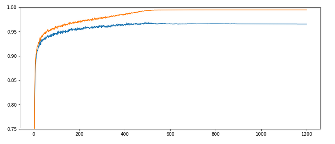
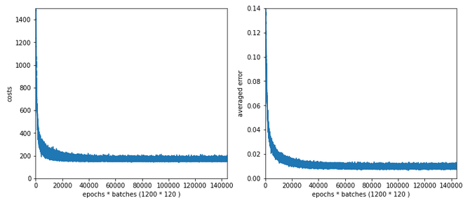
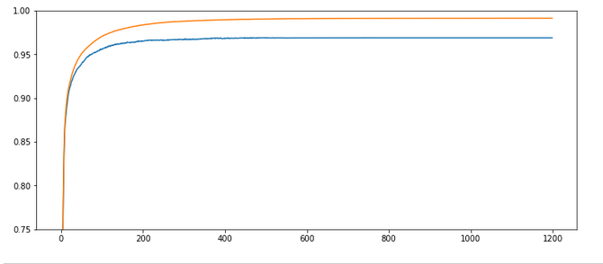
Now we keep the parameters of experiment 5, but we enlarge the batch size – could be helpful to align and deepen the different minima for the different mini-batches – and thus maybe lead to a smoothing. We choose a batch-size of 1200 (i.e. 50 batches instead of 120 in the training set):
Test 6:
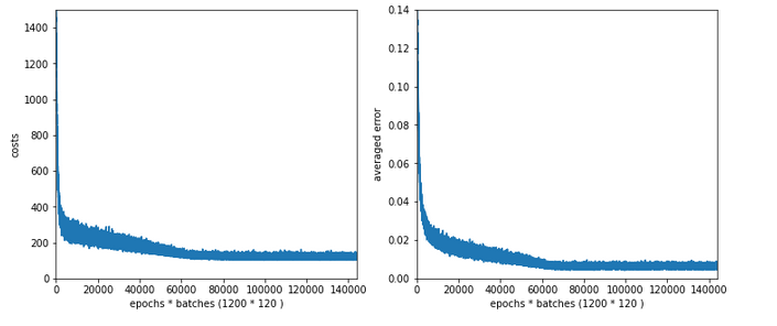
Parameters: learn_rate = 0.001, decrease_rate = 0.00001, mom_rate = 0.00005, n_size_mini_batch = 1200, Lambda2 = 0.2, n_epochs = 2000, initial weights for the matrix first layers L0/L1 [-0.36 0.36], otherwise in [-0.5, 0.5]:
Results: acc_train: 0.959 , acc_test: 0.946, not yet converged after ca. 750 epochs
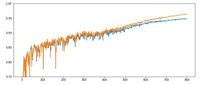
Would you say that enlarging the mini-batch-siz really helped us? I would say: Bigger batch-sizes do not help an algorithm on the verge of trouble! Nope, the structural problems do not disappear.
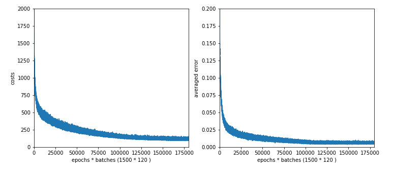
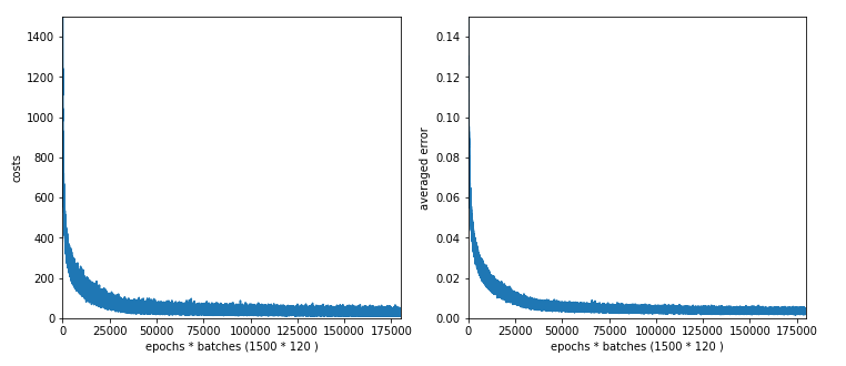
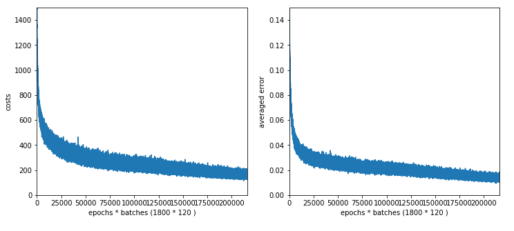
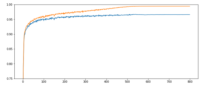
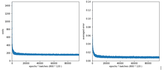
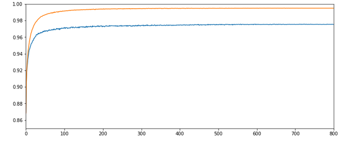
Experiment 7: Reduced learn-rate, increased decrease-rate
Let us face it: For our present state of the MLP-algorithm and the MNIST X-data values directly fed into the input nodes the learn-rate must be chosen significantly smaller to overcome the initial problems of restructuring the weight matrices. So, we give up our trials to work with larger learn-rates – but only for a moment. Let us for confirmation now reduce the initial learning-rate again, but increase the “decrease rate”. At the same time we also decrease the values of the weights.
Test 7:
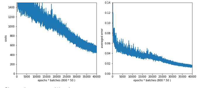
Parameters: learn_rate = 0.0002, decrease_rate = 0.00001, mom_rate = 0.00005, n_size_mini_batch = 500, Lambda2 = 0.2, n_epochs = 1200,initial weights for the matrix first layers L0/L1 [-0.36 0.36] and for the next layers L1/L2 + L2/L3 in [0.08, 0.08]:
Results: acc_train: 0.9943 , acc_test: 0.9655, convergence after ca. 600 epochs
OK, nice again! There is some trouble, but we only need 600 epochs to come to a pretty good accuracy value for the test data set!
Intermediate conclusion
Quite often you may read in literature that a bigger learning rate (often abbreviated with a greek eta) can save computational time in terms of required epochs – as long as convergence is guaranteed. Hmmm – we saw in the tests above that this may not be true under certain conditions. It
is better to say that – depending on the data, the depth of the network and the size of the mini-batches – you may have to control a delicate balance of an initial rate and a rate decline to find an optimum in terms of epochs.
Initial learning rates which are chosen too big together with a too small decrease rate may lead into trouble: the algorithm may get trapped after a few hundred epochs or even stay a long time in some side minimum until it finds a deepening which it really can descent into.
With a smaller learning rate, however, you may find a reasonable path much faster and descent into the minimum much more steadfast and smoothly – in the end requiring remarkably fewer epochs until convergence!
But as we saw with our experiment 4: Even a wiggled start can end up in a pretty good minimum with a really good accuracy. Reducing the learning rate too fast may lead to a circle path with some distance to the minimum. We are talking here about the last < 0.5 percent.
Which minimum level you reach in the end depends on many parameters, but in particular also on the initial weight values. In general setting the initial weight values small enough with respect to the number of nodes on the lower neighbor layer seems to be reasonable.
The sigmoid function – and a major problem
It is time to think a bit deeper before we start more experiments. All in all one does not get rid of the feeling that something profound is wrong with our algorithm or our setup of the experiments. In my youth I have seen similar things in simulations on non-linear physics – and almost always a basic concept was missing or wrongly applied. Time to care about the math.
An important ingredient in the whole learning via back-propagation was the activation function, which due to its non-linearity has an impact on the gradients which we need to calculate. The sigmoid function is a smooth function; but it has some properties which obviously can lead to trouble.
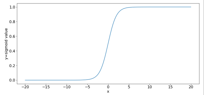
One is that it produces function values pretty close to 1 for arguments x > 15.
sig(10) = 0.9999546021312976
sig(12) = 0.9999938558253978
sig(15) = 0.9999998874648379
sig(20) = 0.9999999979388463
sig(25) = 0.9999999999948910
sig(30) = 0.9999999999999065
So, function values for bigger arguments can almost not be distinguished and resulting gradients during backward propagation will get extremely small. Keeping this in mind we turn towards the initial steps of forward propagation. What happens to our input data there?
We directly present the feature values of the MNIST data images at 784 input nodes in layer L0. The following sketch only shows the basic architecture ofa a MLP; the node numbers do NOT correspond to our present MLP.
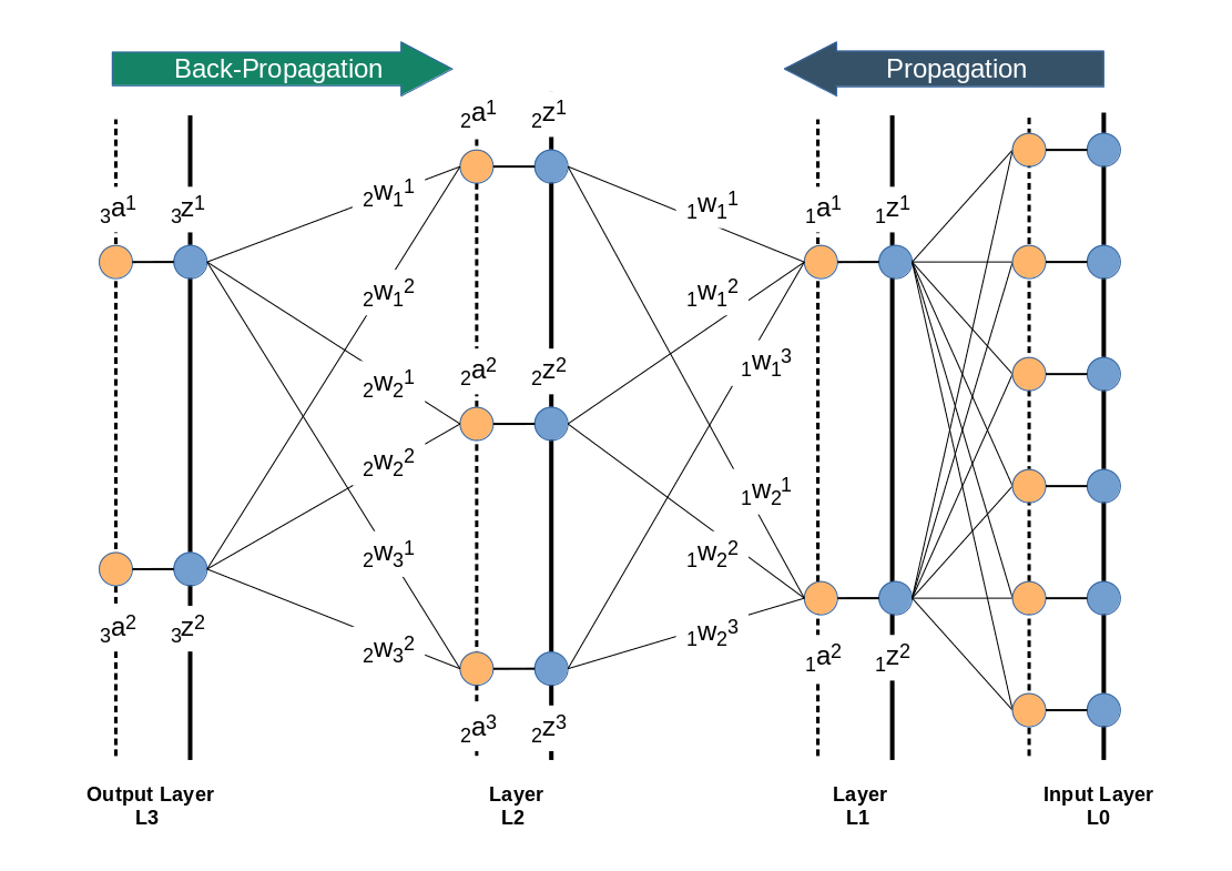
Then we multiply by the weights (randomly chosen initially from some interval) and accumulate 784 contributions at each of the 70 nodes of layer L1. Even if we choose the initial weight values to be in range of [-0.5, +0.5] this will potentially lead to big input values at layer L1 due to summing up all contributions. Thus at the output side of layer L1 our sigmoid function will produce many almost indistinguishable values and pretty small gradients in the first steps. This is certainly not good for a clear adjustment of weights during backward propagation.
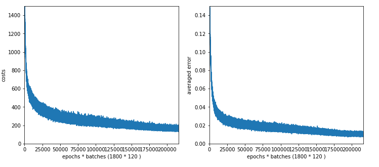
There are two remedies, one can think about:
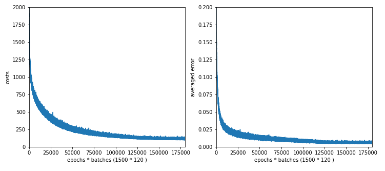
- We should adapt the initial weight values to the number of nodes of the lower
layer in forward propagation direction. A first guess would be something in the range 1.0e-3 for weights between layer L0 and L1 – assuming that ca. 10% of the 784 input features show values around 220. Weights between layers L1 and L2 should be in the range of [-0.05, 0.05] and between layer L2 and L3 in the range [-0.1, 0.1] to prevent maximum values above 5. - We should scale down the input data, i.e. we should normalize them such that they cover a reasonable value range which leads to distinguishable output values of the sigmoid function.
A plot for the first option with a reasonably small learn-rate as in experiment 7 and weights following the 1/sqrt(num_nodes) at every layer (!) is the following :
Quite OK, but not a breakthrough. So, let us look at normalization.
Normalization – Standardization
There are different methods how one can normalize values for a bunch of instances in a set. One basic method is to subtract the minimum value “x_min” of all instances from the value of each instance followed by a division of the difference between the max value (x_max) and the minimum value (x_max – x_min): x => (x – x_min) / (x_max – x_min).
A more clever version – which is called “standardization” – subtracts the mean value “x_mean” of all instances and divides by the standard deviation of the set. The resulting values have a mean of zero and a variance of 1. The advantage of this normalization approach is that it does not react strongly to extreme data values in the set; still it reduces big values to a very moderate scale.
SciKit-Learn provides the second normalization variant as a function with the name “StandardScaler” – this is the reason why we introduced an import statement for this function at the top of this article.
Code modifications to address standardization of the input data
Let us include standardization in our method to handle the input data:
Modifications to function “_method _handle_input_data()”:
    ''' -- Method to handle different types of input data sets --'''
    def _handle_input_data(self):
        '''
        Method to deal with the input data:
        - check if we have a known data set ("mnist" so far)
        - reshape as required
        - analyze dimensions and extract the feature dimension(s)
        '''
        # check for known dataset
        try:
            if (self._my_data_set not in self._input_data_sets ):
                raise ValueError
        except ValueError:
            print("The requested input data" + self._my_data_set + " is not known!" )
            sys.exit()

        # MNIST datasets
        # **************

        # handle the mnist original dataset - is not supported any more
        #if ( self._my_data_set == "mnist"):
        #    mnist = fetch_mldata('MNIST original')
        #    self._X, self._y = mnist["data"], mnist["target"]
        #    print("Input data for dataset " + self._my_data_set + " : \n" + "Original shape of X = " + str(self._X.shape) +
        #      "\n" + "Original shape of y = " + str(self._y.shape))
        #
        # handle the mnist_784 dataset
        if ( self._my_data_set == "mnist_784"):
            mnist2 = fetch_openml('mnist_784', version=1, cache=True, data_home='~/scikit_learn_data')
            self._X, self._y = mnist2["data"], mnist2["
target"]
            print ("data fetched")
            # the target categories are given as strings not integers
            self._y = np.array([int(i) for i in self._y])
            print ("data modified")
            print("Input data for dataset " + self._my_data_set + " : \n" + "Original shape of X = " + str(self._X.shape) +
              "\n" + "Original shape of y = " + str(self._y.shape))

        # handle the mnist_keras dataset
        if ( self._my_data_set == "mnist_keras"):
            (X_train, y_train), (X_test, y_test) = kmnist.load_data()
            len_train =  X_train.shape[0]
            len_test  =  X_test.shape[0]
            X_train = X_train.reshape(len_train, 28*28)
            X_test  = X_test.reshape(len_test, 28*28)

            # Concatenation required due to possible later normalization of all data
            self._X = np.concatenate((X_train, X_test), axis=0)
            self._y = np.concatenate((y_train, y_test), axis=0)
            print("Input data for dataset " + self._my_data_set + " : \n" + "Original shape of X = " + str(self._X.shape) +
              "\n" + "Original shape of y = " + str(self._y.shape))
        #
        # common MNIST handling
        if ( self._my_data_set == "mnist" or self._my_data_set == "mnist_784" or self._my_data_set == "mnist_keras" ):
            self._common_handling_of_mnist()

        # handle IMPORTED datasets
        # **************************+
        if ( self._my_data_set == "imported"):
            if (self._X_import is not None) and (self._y_import is not None):
                self._X = self._X_import
                self._y = self._y_import
            else:
                print("Shall handle imported datasets - but they are not defined")
                sysexit()
        #
        # number of total records in X, y
        # *******************************
        self._dim_X = self._X.shape[0]

        # Give control to preprocessing - has to happen before normalizing and splitting
        # ****************************
        self._preprocess_input_data()
        #
        # Common dataset handling
        # ************************
        # normalization
        if self._b_normalize_X:
            # normalization by sklearn.preprocessing.StandardScaler
            scaler = StandardScaler()
            self._X = scaler.fit_transform(self._X)

        # mixing the training indices - MUST happen BEFORE encoding
        shuffled_index = np.random.permutation(self._dim_X)
        self._X, self._y = self._X[shuffled_index], self._y[shuffled_index]

        # Splitting into training and test datasets
        if self._num_test_records > 0.25 * self._dim_X:
            print("\nNumber of test records bigger than 25% of available data. Too big, we stop." )
            sysexit()
        else:
            num_sep = self._dim_X - self._num_test_records
            self._X_train, self._X_test, self._y_train, self._y_test = self._X[:num_sep], self._X[num_sep:], self._y[:num_sep], self._y[num_sep:]

        # numbers, dimensions
        self._dim_sets = self._y_train.shape[0]
        self._dim_features = self._X_train.shape[1]
        print("\nFinal dimensions of training and test datasets of type " + self._my_data_set +
              " : \n" + "Shape of X_train = " + str(self._X_train.shape) +
              "\n" + "Shape of y_train = " + str(self._y_train.shape) +
              "\n" + "Shape of X_test = " + str(self._X_test.shape) +
              "\n" + "Shape of y_test = " + str(self._y_test.shape)
              )
        print("\nWe have " + str(self._dim_sets) + " data records for training")
        print("Feature dimension is " + str(self._dim_features))


        # encoding the y-values = categories // MUST happen AFTER encoding
        self._get_num_labels()
        self._encode_all_y_labels(self._b_print_test_data)
        #
        ''' Remark: Other input data sets can not yet be handled '''
        return None
#
Well, this looks a bit different compared to our original function. Actually, we perform normalization twice. Once inside the new function “_preprocess_input_data()” and once afterwards.
New function “_preprocess_data()”:
'''----------
    Method to preprocess the input data
    ----------------------------------- '''
    def _preprocess_input_data(self):

        # normalization ahead
        if self._b_normalize_X:
            # normalization by sklearn.preprocessing.StandardScaler
            scaler = StandardScaler()
            self._X = scaler.fit_transform(self._X)

        # Clustering
        if self._b_perform_clustering:
            self._perform_clustering()
            print("\nClustering started")
        else:
            print("\nNo Clustering requested")

        return None
#
The reason is that we have to take into account other transformations of the input data by other methods, too. One of these methods will be clustering, which we shall investigate in a forthcoming article. (For the nervous ones among the readers: The StandardScaler is intelligent enough to avoid divisions by zero means at the second time it is called!)
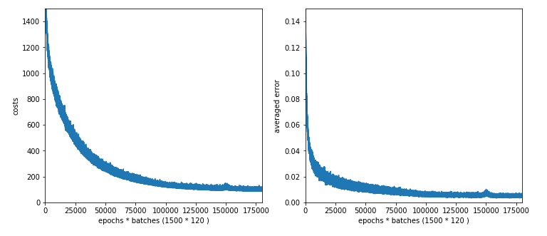
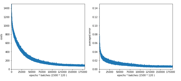
Experiment 8: Standardizes input data, reduced learn-rate, increased decrease-rate and “1/sqrt(nodes)-rule for the initial weights of all layers
We shall call our class My_ANN now with the parameter “b_normalize_X = True”, i.e. we standardize the whole MNIST input data set X before we split it into a training and a test data set.
In addition we apply the rule to set the interval-borders for initial weights to [-1.0/sqrt(num_nodes_layer), 1.0/sqrt(num_nodes_layer)], with “num_nodes_layer” being the number of nodes in the lower layer which the weights act upon during forward propagation.
Test 8:
Parameters: learn_rate = 0.0002, decrease_rate = 0.00001, mom_rate = 0.00005, n_size_mini_batch = 500, Lambda2 = 0.2, n_epochs = 2000, weights at all layers in [- 1.0/sqrt(num_nodes_layer), 1.0/sqrt(num_nodes_layer)]
Results: acc_train: 0.9913 , acc_test: 0.9689, convergence after ca. 650 epochs
Wow, extremely smooth curves now – and we got the highest accuracy so far!
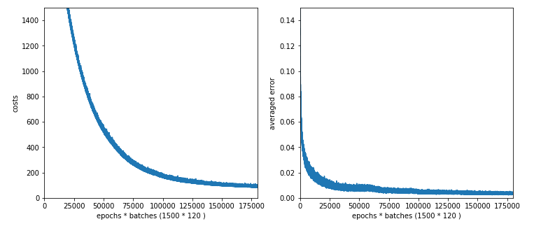
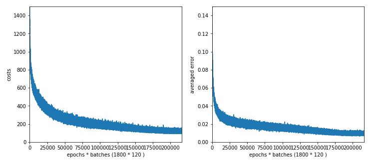
Experiment 9: Standardized input, bigger initial learning rate, enlarged intervals for weight initialization
We get brave again! we enlarge the learning-rate back to 0.001. In addition we enlarge the intervals for a random distribution of initial weights for each layer by a factor of 2 =>- [-2*1.0/sqrt(num_nodes_layer), 2*1.0/sqrt(num_nodes_layer)].
Test 9:
Parameters: learn_rate = 0.001, decrease_rate = 0.00001, mom_rate = 0.00005, n_size_mini_batch = 500, n_epochs = 1200, weights at all layers in [-2*1.0/sqrt(num_nodes_layer), 2*1.
0/sqrt(num_nodes_layer)]
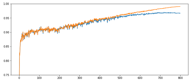
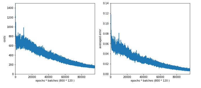
Results: acc_train: 0.9949 , acc_test: 0.9754, convergence after ca. 550-600 epochs
Not such smooth curves as in the previous plot. But WoW again – now we broke the 0.97-threshold – already at an epoch as small as 100!
I admit that a very balanced initial statistical distribution of digit images across the training and the test datasets helped in this specific test run, but only a bit. You will easily and regularly pass a value of 0.972 for the accuracy on the test dataset during multiple consecutive runs. Compared to our reference value of 0.96 this is a solid improvement!
But what is really convincing is the fact the even with a relatively high initial learning rate we see no major trouble on our way to the minimum! I would call this a breakthrough!
Conclusion
We learned today that working with mini-batch training can be tricky. In some cases we may need to control a balance between a sufficiently small initial learning rate and a reasonable reduction rate during training. We also saw that it is helpful to get some control over the weight initialization. The rule to create randomly distributed initial weight values initialization within intervals given by [n*1/sqrt(num_nodes), n*1/sqrt(num_nodes)] appears to be useful.
However, the real lesson of our experiments was that we do our MLP learning algorithm a major favor by normalizing and centering the input data.
At least if the sigmoid function is applied as the activation function at the MLP’s nodes a initial standardization of the input data should always be tested and compared to training runs without standardization.
In the next article of this series
A simple Python program for an ANN to cover the MNIST dataset – XIII – the impact of regularization
we shall have a look at the impact of the regularization parameter Lambda2, which we kept constant, so far. An interesting question in this context is: How does the ratio between the (quadratic) regularization term and the standard cost term in our total loss function change during a training run?
In a further article to come we will then look at a method to detect clusters in the feature parameter space and use related information for gradient descent. The objective of such a step is the reduction of input features and input nodes. Stay tuned!