We proceed with encoding a Python class for a Multilayer Perceptron [MLP] to be able to study at least one simple examples of an artificial neural network [ANN] in detail. During the articles
A simple program for an ANN to cover the Mnist dataset – IV – the concept of a cost or loss function
A simple program for an ANN to cover the Mnist dataset – III – forward propagation
A simple program for an ANN to cover the Mnist dataset – II – initial random weight values
A simple program for an ANN to cover the Mnist dataset – I – a starting point
we came so far that we could apply the “Feed Forward Propagation” algorithm [FFPA] to multiple data records of a mini-batch of training data in parallel. We spoke of a so called vectorized form of the FFPA; we used special Linear Algebra matrix operations of Numpy to achieve the parallel operations. In the last article
A simple program for an ANN to cover the Mnist dataset – IV – the concept of a cost or loss function
I commented on the necessity of a so called “loss function” for the MLP. Although not required for a proper training algorithm we will nevertheless encode a class method to calculate cost values for mini-batches. The behavior of such cost values with training epochs will give us an impression of how good the training algorithm works and whether it actually converges into a minimum of the loss function. As explained in the last article this minimum should correspond to an overall minimum distance of the FFPA results for all training data records from their known correct target values in the result vector space of the MLP.
Before we do the coding for two specific cost or loss functions – namely the “Log Loss“-function and the “MSE“-function, I will briefly point out the difference between standard “*”-operations between multidimensional Numpy arrays and real “dot”-matrix-operations in the sense of Linear Algebra. The latte one follows special rules in multiplying specific elements of both matrices and summing up over the results.
As in all the other articles of this series: This is for beginners; experts will not learn anything new – especially not of the first section.
Element-wise multiplication between multidimensional Numpy arrays in contrast to the “dot”-operation of linear algebra
I would like to point out some aspects of combining two multidimensional Numpy arrays which may be confusing for Python beginners. At least they were for me 🙂 . As a former physicist I automatically expected a “*”-like operation for two multidimensional arrays to perform a matrix operation in the sense of linear algebra. This lead to problems when I tried to understand Python code of others.
Let us assume we have two 2-dimensional arrays A and B. A and B shall be similar in the sense that their shape is identical, i.e. A.shape = B.shape – e.g (784, 60000):
The two matrices each have the same specific number of elements in their different dimensions.
Whenever we operate with multidimensional Numpy arrays with the same same shape we can use the standard operators “+”, “-“, “*”, “/”. These
operators then are applied between corresponding elements of the matrices. I.e., the mathematical operation is applied between elements with the same position along the different dimensional axes in A and B. We speak of an element-wise operation. See the example below.
This means (A * B) is not equivalent to the C = numpy.dot(A, B) operation – which appears in Linear Algebra; e.g. for vector and operator transformations!
The”dot()”-operation implies a special operation: Let us assume that the shape of A[i,j,v] is
A.shape = (p,q,y)
and the shape of B[k,w,m] is
B.shape = (r,z,s)
with
y = z .
Then in the “dot()”-operation all elements of a dimension “v” of A[i,j,v] are multiplied with corresponding elements of the dimension “w” of B[k,w,m] and then the results summed up.
dot(A, B)[i,j,k,m] = sum(A[i,j,:] * B[k,:,m])
The “*” operation in the formula above is to be interpreted as a standard multiplication of array elements.
In the case of A being a 2-dim array and B being a 1-dimensional vector we just get an operation which could – under certain conditions – be interpreted as a typical vector transformation in a 2-dim vector space.
So, when we define two Numpy arrays there may exist two different methods to deal with array-multiplication: If we have two arrays with the same shape, then the “*”-operation means an element-wise multiplication of the elements of both matrices. In the context of ANNs such an operation may be useful – even if real linear algebra matrix operations dominate the required calculations. The first “*”-operation will, however, not work if the array-shapes deviate.
The “numpy.dot(A, B)“-operation instead requires a correspondence of the last dimension of matrix A with the second to last dimension of matrix B. Ooops – I realize I just used the expression “matrix” for a multidimensional Numpy array without much thinking. As said: “matrix” in linear algebra has a connotation of a transformation operator on vectors of a vector space. Is there a difference in Numpy?
Yes, there is, indeed – which may even lead to more confusion: We can apply the function numpy.matrix()
A = numpy.matrix(A),
B = numpy.matrix(B)
then the “*”-operator will get a different meaning – namely that of numpy.dot(A,B):
A * B = numpy.dot(A, B)
So, better read Python code dealing with multidimensional arrays rather carefully ….
To understand this better let us execute the following operations on some simple examples in a Jupyter cell:
A1 = np.ones((5,3))
A1[:,1] *= 2
A1[:,2] *= 4
print("\nMatrix A1:\n")
print(A1)


A2= np.random.randint(1, 10, 5*3)
A2 = A2.reshape(5,3)
# A2 = A2.reshape(3,5)
print("\n Matrix A2 :\n")
print(A2)


A3 = A1 * A2
print("\n\nA3:\n")
print(A3)

A4 = np.dot(A1, A2.T)
print("\n\nA4:\n")
print(A4)

A5 = np.matrix(A1)
A6 = np.matrix(A2)

A7 = A5 * A6.T
print("\n\nA7:\n")
print(A7)

A8 = A5 * A6
We get the following output:
Matrix A1:

[[1. 2. 4.]
 [1. 2. 4.]
 [1. 2. 4.]
 [1. 2. 4.]
 [1. 2. 4.]]

 Matrix A2 :

[[6 8 9]
 [9 1 6]
 [8 8 9]
 [2 8 3]
 [5 8 8]]


A3:

[[ 6. 16. 36.]
 [ 9.  2. 24.]
 [ 8. 16. 36.]
 [ 2. 16. 12.]
 [
 5. 16. 32.]]


A4:

[[58. 35. 60. 30. 53.]
 [58. 35. 60. 30. 53.]
 [58. 35. 60. 30. 53.]
 [58. 35. 60. 30. 53.]
 [58. 35. 60. 30. 53.]]


A7:

[[58. 35. 60. 30. 53.]
 [58. 35. 60. 30. 53.]
 [58. 35. 60. 30. 53.]
 [58. 35. 60. 30. 53.]
 [58. 35. 60. 30. 53.]]

---------------------------------------------------------------------------
ValueError                                Traceback (most recent call last)
<ipython-input-10-4ea2dbdf6272> in <module>
     28 print(A7)
     29
---> 30 A8 = A5 * A6
     31

/projekte/GIT/ai/ml1/lib/python3.6/site-packages/numpy/matrixlib/defmatrix.py in __mul__(self, other)
    218         if isinstance(other, (N.ndarray, list, tuple)) :
    219             # This promotes 1-D vectors to row vectors
--> 220             return N.dot(self, asmatrix(other))
    221         if isscalar(other) or not hasattr(other, '__rmul__') :
    222             return N.dot(self, other)

<__array_function__ internals> in dot(*args, **kwargs)

ValueError: shapes (5,3) and (5,3) not aligned: 3 (dim 1) != 5 (dim 0)
This example obviously demonstrates the difference of an multiplication operation on multidimensional arrays and a real matrix “dot”-operation. Note especially how the “*” operator changed when we calculated A7.
If we instead execute the following code
A1 = np.ones((5,3))
A1[:,1] *= 2
A1[:,2] *= 4
print("\nMatrix A1:\n")
print(A1)


A2= np.random.randint(1, 10, 5*3)
#A2 = A2.reshape(5,3)
A2 = A2.reshape(3,5)
print("\n Matrix A2 :\n")
print(A2)

A3 = A1 * A2
print("\n\nA3:\n")
print(A3)
we directly get an error:
Matrix A1:

[[1. 2. 4.]
 [1. 2. 4.]
 [1. 2. 4.]
 [1. 2. 4.]
 [1. 2. 4.]]

 Matrix A2 :

[[5 8 7 3 8]
 [4 4 8 4 5]
 [8 1 9 4 8]]

---------------------------------------------------------------------------
ValueError                                Traceback (most recent call last)
<ipython-input-12-c4d3ffb1e683> in <module>
     13
     14
---> 15 A3 = A1 * A2
     16 print("\n\nA3:\n")
     17 print(A3)

ValueError: operands could not be broadcast together with shapes (5,3) (3,5)
As expected!
Cost calculation for our ANN
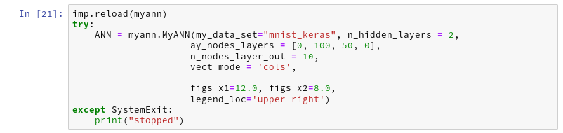
As we want to be able to use different types of cost/loss functions we have to introduce new corresponding parameters in the class’s interface. So we update the “__init__()”-function:
def __init__(self,
my_data_set = "mnist",
n_hidden_layers = 1,
ay_nodes_layers = [0, 100, 0], # array which should have as much elements as n_hidden + 2
n_nodes_layer_out = 10, # expected number of nodes in output layer
my_activation_function = "sigmoid",
my_out_function = "sigmoid",
my_loss_function = "LogLoss",
n_size_mini_batch = 50, # number of data elements in a mini-batch
n_epochs = 1,
n_max_batches = -1, # number of mini-batches to use during epochs - > 0 only for testing
# a negative value uses all mini-batches
lambda2_reg = 0.1, # factor for quadratic regularization term
lambda1_reg = 0.0, # factor for linear regularization term
vect_mode = 'cols',
figs_x1=12.0, figs_x2=8.0,
legend_loc='upper
right',
b_print_test_data = True
):
'''
Initialization of MyANN
Input:
data_set: type of dataset; so far only the "mnist", "mnist_784" datsets are known
We use this information to prepare the input data and learn about the feature dimension.
This info is used in preparing the size of the input layer.
n_hidden_layers = number of hidden layers => between input layer 0 and output layer n
ay_nodes_layers = [0, 100, 0 ] : We set the number of nodes in input layer_0 and the output_layer to zero
Will be set to real number afterwards by infos from the input dataset.
All other numbers are used for the node numbers of the hidden layers.
n_nodes_out_layer = expected number of nodes in the output layer (is checked);
this number corresponds to the number of categories NC = number of labels to be distinguished
my_activation_function : name of the activation function to use
my_out_function : name of the "activation" function of the last layer which produces the output values
my_loss_function : name of the "cost" or "loss" function used for optimization
n_size_mini_batch : Number of elements/samples in a mini-batch of training data
The number of mini-batches will be calculated from this
n_epochs : number of epochs to calculate during training
n_max_batches : > 0: maximum of mini-batches to use during training
< 0: use all mini-batches
lambda_reg2: The factor for the quadartic regularization term
lambda_reg1: The factor for the linear regularization term
vect_mode: Are 1-dim data arrays (vctors) ordered by columns or rows ?
figs_x1=12.0, figs_x2=8.0 : Standard sizing of plots ,
legend_loc='upper right': Position of legends in the plots
b_print_test_data: Boolean variable to control the print out of some tests data
'''
# Array (Python list) of known input data sets
self._input_data_sets = ["mnist", "mnist_784", "mnist_keras"]
self._my_data_set = my_data_set
# X, y, X_train, y_train, X_test, y_test
# will be set by analyze_input_data
# X: Input array (2D) - at present status of MNIST image data, only.
# y: result (=classification data) [digits represent categories in the case of Mnist]
self._X = None
self._X_train = None
self._X_test = None
self._y = None
self._y_train = None
self._y_test = None
# relevant dimensions
# from input data information; will be set in handle_input_data()
self._dim_sets = 0
self._dim_features = 0
self._n_labels = 0 # number of unique labels - will be extracted from y-data
# Img sizes
self._dim_img = 0 # should be sqrt(dim_features) - we assume square like images
self._img_h = 0
self._img_w = 0
# Layers
# ------
# number of hidden layers
self._n_hidden_layers = n_hidden_layers
# Number of total layers
self._n_total_layers = 2 + self._n_hidden_layers
# Nodes for hidden layers
self._ay_nodes_layers = np.array(ay_nodes_layers)
# Number of nodes in output
layer - will be checked against information from target arrays
self._n_nodes_layer_out = n_nodes_layer_out
# Weights
# --------
# empty List for all weight-matrices for all layer-connections
# Numbering :
# w[0] contains the weight matrix which connects layer 0 (input layer ) to hidden layer 1
# w[1] contains the weight matrix which connects layer 1 (input layer ) to (hidden?) layer 2
self._ay_w = []
# Arrays for encoded output labels - will be set in _encode_all_mnist_labels()
# -------------------------------
self._ay_onehot = None
self._ay_oneval = None
# Known Randomizer methods ( 0: np.random.randint, 1: np.random.uniform )
# ------------------
self.__ay_known_randomizers = [0, 1]
# Types of activation functions and output functions
# ------------------
self.__ay_activation_functions = ["sigmoid"] # later also relu
self.__ay_output_functions = ["sigmoid"] # later also softmax
# Types of cost functions
# ------------------
self.__ay_loss_functions = ["LogLoss", "MSE" ] # later also othr types of cost/loss functions
# the following dictionaries will be used for indirect function calls
self.__d_activation_funcs = {
'sigmoid': self._sigmoid,
'relu': self._relu
}
self.__d_output_funcs = {
'sigmoid': self._sigmoid,
'softmax': self._softmax
}
self.__d_loss_funcs = {
'LogLoss': self._loss_LogLoss,
'MSE': self._loss_MSE
}
# The following variables will later be set by _check_and set_activation_and_out_functions()
self._my_act_func = my_activation_function
self._my_out_func = my_out_function
self._my_loss_func = my_loss_function
self._act_func = None
self._out_func = None
self._loss_func = None
# list for cost values of mini-batches during training
# The list will later be split into sections for epochs
self._ay_cost_vals = []
# number of data samples in a mini-batch
self._n_size_mini_batch = n_size_mini_batch
self._n_mini_batches = None # will be determined by _get_number_of_mini_batches()
# number of epochs
self._n_epochs = n_epochs
# maximum number of batches to handle (<0 => all!)
self._n_max_batches = n_max_batches
# regularization parameters
self._lambda2_reg = lambda2_reg
self._lambda1_reg = lambda1_reg
# paramter to allow printing of some test data
self._b_print_test_data = b_print_test_data
# Plot handling
# --------------
# Alternatives to resize plots
# 1: just resize figure 2: resize plus create subplots() [figure + axes]
self._plot_resize_alternative = 1
# Plot-sizing
self._figs_x1 = figs_x1
self._figs_x2 = figs_x2
self._fig = None
self._ax = None
# alternative 2 does resizing and (!) subplots()
self.initiate_and_resize_plot(self._plot_resize_alternative)
# ***********
# operations
# ***********
# check and handle input data
self._handle_input_data()
# set the ANN structure
self._set_ANN_structure()
# Prepare epoch and batch-handling - sets mini-batch index array, too
self._prepare_epochs_and_batches()
# perform training
start_c = time.perf_counter()
self._fit(b_print=False, b_measure_batch_time=False)
end_c = time.perf_counter()
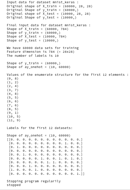
print('\n\n ------')
print('Total training Time_CPU: ', end_c - start_c)
print("\nStopping program regularily")
sys.exit()
#
The way of accessing a method/function by a parameterized “name”-string should already be familiar from other methods. The method with the given name must of course exist in the Python module; otherwise already Eclipse#s PyDev we display errors.
    '''-- Method to set the loss function--'''
    def _check_and_set_loss_function(self):
        # check for known loss functions
        try:
            if (self._my_loss_func not in self.__d_loss_funcs ):
                raise ValueError
        except ValueError:
            print("\nThe requested loss function " + self._my_loss_func + " is not known!" )
            sys.exit()

        # set the function to variables for indirect addressing
        self._loss_func = self.__d_loss_funcs[self._my_loss_func]

        if self._b_print_test_data:
            z = 2.0
            print("\nThe loss function of the ANN/MLP was defined as \""  + self._my_loss_func + '"')
        '''
        '''
        return None
#
The “Log Loss” function
The “LogLoss”-function has a special form. If “a_i” characterizes the FFPA result for a special training record and “y_i” the real known value for this record then we calculate its contribution to the costs as:
Loss = SUM_i [- y_i * log(a_i) – (1 – y_i)*log(1 – a_i)]
This loss function has its justification in statistical considerations – for which we assume that our output function produces a kind of probability distribution. Please see the literature for more information.
Now, due to the encoded result representation over 10 different output dimensions in the MNIST case, corresponding to 10 nodes in the output layer; see the second article of this series, we know that a_i and y_i would be 1-dimensional arrays for each training data record. However, if we vectorize this by treating all records of a mini-batch in parallel we get 2-dim arrays. Actually, we have already calculated the respective arrays in the second to last article.
The rows (1st dim) of a represent the output nodes (training data records, the columns (2nd dim) of a represent the results of the FFPA-result values, which due to our output function have values in the interval ]0.0, 1.0].
The same holds for y – with the difference, that 9 of the values in the rows are 0 and exactly one is 1 for a training record.
The “*” multiplication thus can be done via a normal element-wise array “multiplication” on the given 2-dim arrays of our code.
a = ay_ANN_out
y = ay_y_enc
Numpy offers a function “numpy.sum(M)” for a multidimensional array M, which just sums up all element values. The result is of course a simple scalar.
This information should be enough to understand the following new method:
    ''' method to calculate the logistic regression loss function '''
    def _loss_LogLoss(self, ay_y_enc, ay_ANN_out, b_print = False):
        '''
        Method which calculates LogReg loss function in a vectorized form on multidimensional Numpy arrays
        '''
        b_test = False

        if b_print:
            print("From LogLoss: shape of ay_y_enc =  " + str(ay_y_enc.shape))
            print("From LogLoss: shape of ay_ANN_out =  " + str(ay_
ANN_out.shape))
            print("LogLoss: ay_y_enc = ", ay_y_enc)
            print("LogLoss: ANN_out = \n", ay_ANN_out)
            print("LogLoss: log(ay_ANN_out) =  \n", np.log(ay_ANN_out) )

        # The following means an element-wise (!) operation between matrices of the same shape!
        Log1 = -ay_y_enc * (np.log(ay_ANN_out))
        # The following means an element-wise (!) operation between matrices of the same shape!
        Log2 = (1 - ay_y_enc) * np.log(1 - ay_ANN_out)

        # the next operation calculates the sum over all matrix elements
        # - thus getting the total costs for all mini-batch elements
        cost = np.sum(Log1 - Log2)

        #if b_print and b_test:
            # Log1_x = -ay_y_enc.dot((np.log(ay_ANN_out)).T)
            # print("From LogLoss: L1 =   " + str(L1))
            # print("From LogLoss: L1X =  " + str(L1X))

        if b_print:
            print("From LogLoss: cost =  " + str(cost))

        # The total costs is just a number (scalar)
        return cost
The Mean Square Error [MSE] cost function
Although not often used for classification tasks (but more for regression problems) this loss function is so simple that we encode it on the fly. Here we just calculate something like a mean quadratic error:
Loss = 9.5 * SUM_i [ (y_i – a_i)**2 ]
This loss function is convex by definition and leads to the following method code:
    ''' method to calculate the MSE loss function '''
    def _loss_MSE(self, ay_y_enc, ay_ANN_out, b_print = False):
        '''
        Method which calculates LogReg loss function in a vectorized form on multidimensional Numpy arrays
        '''
        if b_print:
            print("From loss_MSE: shape of ay_y_enc =  " + str(ay_y_enc.shape))
            print("From loss_MSE: shape of ay_ANN_out =  " + str(ay_ANN_out.shape))
            #print("LogReg: ay_y_enc = ", ay_y_enc)
            #print("LogReg: ANN_out = \n", ay_ANN_out)
            #print("LogReg: log(ay_ANN_out) =  \n", np.log(ay_ANN_out) )

        cost = 0.5 * np.sum( np.square( ay_y_enc - ay_ANN_out ) )

        if b_print:
            print("From loss_MSE: cost =  " + str(cost))

        return cost
#
Regularization terms
Regularization is a means against overfitting during training. The trick is that the cost function is enhanced by terms which include sums of linear or quadratic terms of all weights of all layers. This enforces that the weights themselves get minimized, too, in the search for a minimum of the loss function. The less degrees of freedom there are the less the chance of overfitting …
In the literature (see the book hints in the last article) you find 2 methods for regularization – one with quadratic terms of the weights – the so called “Ridge-Regression” – and one based on a sum of absolute values of the weights – the so called “Lasso regression”. See the books of Geron and Rashka for more information.
Loss = SUM_i [- y_i * log(a_i) – (1 – y_i)*log(1 – a_i)]
+ lambda_2 * SUM_layer [ SUM_nodes [ (w_layer_nodes)**2 ] ]
+ lambda_1 * SUM_layer [ SUM_nodes [ |w_layer_nodes| ] ]
Note that we included already two factors “lambda_2” and “lamda_1” by which the regularization terms are multiplied and added to the cost/loss function in the “__init__”-method.
The two related methods are easy to understand:
    ''' method do calculate the quadratic regularization term for the loss function '''
    def _regularize_by_L2(self, b_print=False):

'''
        The L2 regularization term sums up all quadratic weights (without the weight for the bias)
        over the input and all hidden layers (but not the output layer
        The weight for the bias is in the first column (index 0) of the weight matrix -
        as the bias node's output is in the first row of the output vector of the layer
        '''
        ilayer = range(0, self._n_total_layers-1) # this excludes the last layer
        L2 = 0.0
        for idx in ilayer:
            L2 += (np.sum( np.square(self._ay_w[idx][:, 1:])) )
        L2 *= 0.5 * self._lambda2_reg
        if b_print:
            print("\nL2: total L2 = " + str(L2) )
        return L2
#
    ''' method do calculate the linear regularization term for the loss function '''
    def _regularize_by_L1(self, b_print=False):
        '''
        The L1 regularization term sums up all weights (without the weight for the bias)
        over the input and all hidden layers (but not the output layer
        The weight for the bias is in the first column (index 0) of the weight matrix -
        as the bias node's output is in the first row of the output vector of the layer
        '''
        ilayer = range(0, self._n_total_layers-1) # this excludes the last layer
        L1 = 0.0
        for idx in ilayer:
            L1 += (np.sum( self._ay_w[idx][:, 1:]))
        L1 *= 0.5 * self._lambda1_reg
        if b_print:
            print("\nL1: total L1 = " + str(L1))
        return L1
#
Why do we not start with index “0” in the weight arrays – self._ay_w[idx][:, 1:]?
The reason is that we do not include the Bias-node in these terms. The weight at the bias nodes of the layers is not varied there during optimization!
Note: Normally we would expect a factor of 1/m, with “m” being the number of records in a mini-batch, for all the terms discussed above. Such a constant factor does not hamper the principal procedure – if we omit it consistently also for for the regularization terms discussed below. It can be taken care of by choosing smaller “lambda”s and a smaller step size during optimization.
Inclusion of the loss function calculations within the handling of mini-batches
For our approach with mini-batches (i.e. an approach between pure stochastic and full batch handling) we have to include the cost calculation in our method “_handle_mini_batch()” to handle mini-batches. Method “_handle_mini_batch()” is modified accordingly:
    ''' -- Method to deal with a batch -- '''
    def _handle_mini_batch(self, num_batch = 0, b_print_y_vals = False, b_print = False):
        '''
        For each batch we keep the input data array Z and the output data A (output of activation function!)
        for all layers in Python lists
        We can use this as input variables in function calls - mutable variables are handled by reference values !
        We receive the A and Z data from propagation functions and proceed them to cost and gradient calculation functions

        As an initial step we define the Python lists ay_Z_in_layer and ay_A_out_layer
        and fill in the first input elements for layer L0
        '''
        ay_Z_in_layer  = [] # Input vector in layer L0;  result of a matrix operation in L1,...
        ay_A_out_layer = [] # Result of activation function

        #print("num_batch = " + str(num_batch))
        #print("len of ay_mini_batches = " + str(len(self._ay_mini_batches)))
        #print("_ay_mini_batches[0] = ")
        #print(self._ay_mini_batches[num_batch])

        # Step 1: Special treatment of the ANN's input Layer L0
        # Layer L0: Fill in the input vector for the ANN'
s input layer L0
        ay_idx_batch = self._ay_mini_batches[num_batch]
        ay_Z_in_layer.append( self._X_train[ay_idx_batch] ) # numpy arrays can be indexed by an array of integers
        #print("\nPropagation : Shape of X_in = ay_Z_in_layer = " + str(ay_Z_in_layer[0].shape))
        if b_print_y_vals:
            print("\n idx, expected y_value of Layer L0-input :")
            for idx in self._ay_mini_batches[num_batch]:
                print(str(idx) + ', ' + str(self._y_train[idx]) )

        # Step 2: Layer L0: We need to transpose the data of the input layer
        ay_Z_in_0T       = ay_Z_in_layer[0].T
        ay_Z_in_layer[0] = ay_Z_in_0T

        # Step 3: Call the forward propagation method for the mini-batch data samples
        self._fw_propagation(ay_Z_in = ay_Z_in_layer, ay_A_out = ay_A_out_layer, b_print = b_print)

        if b_print:
            # index range of layers
            ilayer = range(0, self._n_total_layers)
            print("\n ---- ")
            print("\nAfter propagation through all " + str(self._n_total_layers) + " layers: ")
            for il in ilayer:
                print("Shape of Z_in of layer L" + str(il) + " = " + str(ay_Z_in_layer[il].shape))
                print("Shape of A_out of layer L" + str(il) + " = " + str(ay_A_out_layer[il].shape))


        # Step 4: To be done: cost calculation for the batch
        ay_y_enc = self._ay_onehot[:, ay_idx_batch]
        ay_ANN_out = ay_A_out_layer[self._n_total_layers-1]
        # print("Shape of ay_ANN_out = " + str(ay_ANN_out.shape))

        total_costs_batch = self._calculate_loss_for_batch(ay_y_enc, ay_ANN_out, b_print = False)
        self._ay_cost_vals.append(total_costs_batch)

        # Step 5: To be done: gradient calculation via back propagation of errors
        # Step 6: Adjustment of weights

        # try to accelerate garbage handling
        if len(ay_Z_in_layer) > 0:
            del ay_Z_in_layer
        if len(ay_A_out_layer) > 0:
            del ay_A_out_layer

        return None
#
Note that we save the cost values of every batch in the 1-dim array “self._ay_cost_vals”. This array can later on easily be split into arrays for epochs.
The whole process must be supplemented by a method which does the real cost value calculation:
    ''' -- Main Method to calculate costs -- '''
    def _calculate_loss_for_batch(self, ay_y_enc, ay_ANN_out, b_print = False, b_print_details = False ):
        '''
        Method which calculates the costs including regularization terms
        The cost function is called according to an input parameter of the class
        '''
        pure_costs_batch = self._loss_func(ay_y_enc, ay_ANN_out, b_print = False)

        if ( b_print and b_print_details ):
            print("Calc_Costs: Shape of ay_ANN_out = " + str(ay_ANN_out.shape))
            print("Calc_Costs: Shape of ay_y_enc = " + str(ay_y_enc.shape))
        if b_print:
            print("From Calc_Costs: pure costs of a batch =  " + str(pure_costs_batch))

        # Add regularitzation terms - L1: linear reg. term, L2: quadratic reg. term
        # the sums over the weights (squared) have to be performed for each batch again due to intermediate corrections
        L1_cost_contrib = 0.0
        L2_cost_contrib = 0.0
        if self._lambda1_reg > 0:
            L1_cost_contrib = self._regularize_by_L1( b_print=False )
        if self._lambda2_reg > 0:
            L2_cost_contrib = self._regularize_by_L2( b_print=False )

        total_costs_batch = pure_costs_batch + L1_cost_contrib + L2_cost_contrib
        return total_costs_batch
#
Conclusion
By the steps
discussed above we completed the inclusion of a cost value calculation in our class for every step dealing with a mini-batch during training. All cost values are saved in a Python list for later evaluation. The list can later be split with respect to epochs.
In contrast to the FFP-algorithm all array-operations required in this step were simple element-wise operations and summations over all array-elements.
Cost value calculation obviously is simple and pretty fast regarding CPU-consumption! Just test it yourself!
In the next article we shall analyze the mathematics behind the calculation of the partial derivatives of our cost-function with respect to the many weights at all nodes of the different layers. We shall see that the gradient calculation reduces to remarkable simple formulas describing a kind of back-propagation of the error terms [y_i – a_i] through the network.
We will not be surprised that we need to involve some real matrix operations again as in the FFPA !