For beginners both in Python and Machine Learning [ML] the threshold to do some real programming and create your own Artificial Neural Network [ANN] seems to be relatively high. Well, some readers might say: Why program an ANN by yourself at a basic Python level at all when Keras and TensorFlow [TF] are available? Answer: For learning! And eventually to be able to do some things TF has not been made for. And as readers of this blog will see in the future, I have some ideas along this line …
So I thought, just let me set up a small Python3 and Numpy based program to create a simple kind of ANN – a “Multilayer Perceptron” [MLP] – and train it for the MNIST dataset. I expected that my readers and I myself would earn something on various methods used in ML during our numerical experiments. Well, we shall see ..-
Regarding ANN-theory I take a brutal shortcut and assume that my readers are already acquainted with the following topics:
- what simple neural networks with “hidden” layers look like and what its weights are,
- what a “cost function” is and how the gradient descent method works,
- what logistic regression is and what the cost function J for it looks like,
- why we need the back propagation of deviations from known values and why it gives you the required partial derivatives of a typical cost function with respect to an ANN’s “weights”,
- what a mini-batch approach to weight optimization is.
I cannot spare you the effort of studying most of these topics in advance. Otherwise I would have to write an introductory book on ML myself. [I would do, but you need to give me a sponsor 🙂 ] But even if you are not fully acquainted with all the named topics: I shall briefly comment on each and every of the points in the forthcoming articles. The real basics are, however, much better and more precisely documented in the literature; e.g. in the books of Geron and Rashka (see the references at the end of this article). I recommend to read one of these books whilst we move on with a sequence of steps to build the basic code for our MLP.
We need a relatively well defined first objective for the usage of our ANN. We shall concentrate on classification tasks. As a first example we shall use the conventional MNIST data set. The MNIST data set consists of images of handwritten numbers with 28×28 pixels [px]. It is a standard data set used in many elementary courses on ML. The challenge for our ANN is that it should be able to recognize hand-written digits from a digitized gray-color image after some training.
Note that this task does NOT require the use of a fully fletched multi-layer MLP. “Stochastic Gradient Descent”-approaches for a pure binary classificator to determine (linear) separation surfaces in combination with a “One-versus-All” strategy for multi-category-classification may be sufficient. See chapters 3 to 5 in the book of Geron for more information.
Regarding the build up of the ANN program, I basically follow an approach described by S. Raschka in his book (see the second to last section for a reference). However, at multiple points I take my freedom to organize the code differently and comment in my own way … I am only a beginner in Python; I hope my insights are helpful for others in the same situation.
In any case you should make yourself familiar with numpy arrays and their “shapes”. I assume that you understand the multidimensional structure of Numpy arrays ….
Wording
To avoid confusion, I use the following wording and synonyms:
Category: Each input data element is associated with a category to which it belongs. In our case a category
corresponds to a “digit”. The classification algorithm (here: the MLP) may achieve an ability to predict the association of an unknown MNIST like input data sample with its correct category. It should – after some training – detect the (non-linear) separation interfaces for categories in a multidimensional feature space. In the case of MNIST we speak about ten categories corresponding to 10 digits, including zero.
Label: A category may be described by a label. Training data may provide a so called “target label array” _y_train for all input data. We must be prepared to transform target labels for input data into a usable form for an ANN, i.e. into a vectorized form, which selects a specific category out of many. This process is called “label encoding”.
Input data set: A complete “set” of input data. Such a set consists of individual “elements” or “records“. Another term which we I shall frequently use for such an element is a “sample“. The MNIST input set of training data consists of 60000 records or samples – which we provide via an array _X_train. The array is two dimensional as each sample consists of values more multiple properties.
Feature: A sample of the input data set may be equivalent to a mathematical vector, whose elements specify (numerical) values for multiple properties – so called “features” – of a sample. Thus, input samples correspond to points in a multidimensional feature space.
Output data set: A complete set of output data after a so called “propagation” through the ANN for the input data set. “Propagation”means a series of defined mathematical transformations of the original features data of the input sample. The number of samples or records in the output data sets is equal to the number of records in the input data set. The output set will be represented by a Numpy array “_ay_ANN_out“.
A data record or sample of the input data set: One distinct element of the input data set (and its array). Note that such an element itself may be a multidimensional array covering all features in a distinct form. Such arrays represents a so called “tensor”.
A data record of the output data set: One distinct element of the output data set. Note that such an element itself may be an array covering all possible categories in a distinct form. E.g., we may be given a “probability” for each category – which allows us to decide with which of the categories we should associate the output element.
A simple MLP network – layers, nodes, weights
An AN network is composed of a series of horizontally and/or vertically arranged layers with nodes. The nodes represent the artificial neurons. A MLP is an ANN which has a rather simple structure: It consists of an input layer, multiple sequential intermediate “hidden” layers, and an output layer. All nodes of a specific layer are connected with all nodes of neighboring (!) layers, only. We speak of a “dense” or fully “connected layer” structure.
The simplifying sketch below displays an ANN with just three sequentially arranged layers – an input layer, a “hidden” middle layer and an output layer.
Note that in general there can be (many) more hidden layers than just one. Note also that modern ANNs (e.g. Convoluted Networks) may have a much more complicated topological structure with hundreds of layers. There may also be
cascaded networks where a specific layer has connections to many more than just the neighbor layers.
Input layer and its number of nodes
To feed input data into the MLP we need an “input layer” with sufficient input nodes. How many? Well, this depends on the number of features your data set represents. In the MNIST case a sample image contains 28×28 pixels. For each pixel with a gray value (integer number between 0 and 256) given. So a typical image represents 28×28 = 768 different “features” – i.e. 786 numbers for “gray”-values between 0 and 255. We need as many input nodes in our MLP to represent the full image information by the input layer.
For other input data the number of features may be different; in addition features my follow a multidimensional order or organization which first must be “flattened” out in one dimension. The number of input nodes must then be adjusted accordingly. The number of input nodes should, therefore, be a parameter or be derived from information on the type of input data. The way of how you map complicated and structured features to input layers and whether you map all data to a one dimensional input vector is a question one should think about carefully. (Most people today treat e.g. a time dimension of input data as just a special form of a feature – I regard this as questionable in some cases, but this is beyond this article series …)
For our MLP we always assume a mapping of features to a flat one dimensional vector like structure.
Output layer and its number of nodes
We shall use our MLP for classification tasks in the beginning. We, therefore, assume that the output of the ANN should allow for the distinction between “strong>NC” different categories an input data set can belong to. In case of the MNIST dataset we can distinguish between 10 different digits. Thus an output layer must in this case comprise 10 different nodes. To be able to cover other data sets with a different number of categories the number of output nodes must be a parameter of our program, too.
How we indicate the association of a (transformed) sample at the output layer to a category numerically – by a probability number between “0” and “1” or just a “1” at the right category and zeros otherwise – can be a matter of discussion. It is also a question of the cost function we wish to use. We will come back to this point in later articles.
The numbers of “hidden layers” and their nodes
We want the numbers of nodes on “hidden layers” to be parameters for our program. For simple data as MNIST images we do not need big networks, but we want to be able to play around a bit with 1 up to 3 layers. (For an ANN to recognize hand written MNIST digits an input layer “L0” and only one hidden layer “L1” before an output layer “L2” are fully sufficient. Nevertheless in most of our experiments we will actually use 2 hidden layers. There are three reasons: You can approximate any continuous function with two hidden layers (with a special non-linear activation function; see below) and an output layer (with just a linear output function). The other reason is that the full mathematical complexity of “learning” of a MLP appears with two hidden layers (see a later article).
Activation and output functions
The nodes in hidden layers use a so called “activation function” to transform aggregated input from different feeding nodes of the previous layer into one distinct value within a defined interval – e.g. between -1 and 1. Again, we should be prepared to have a program parameter to choose between different “activation functions”.
We should be aware of the fact that the nodes of the output layers need special consideration as the “activation function” there
produces the final output – which in turn must allow for a distinction of categories. This may lead to a special form – e.g. a kind of probability function. So, the type of the “output function” should also be regarded as variable parameter.
A Python class for our ANN and its interface
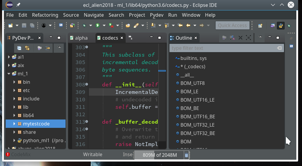
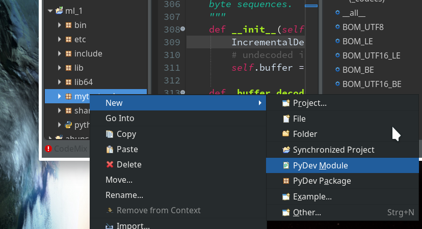
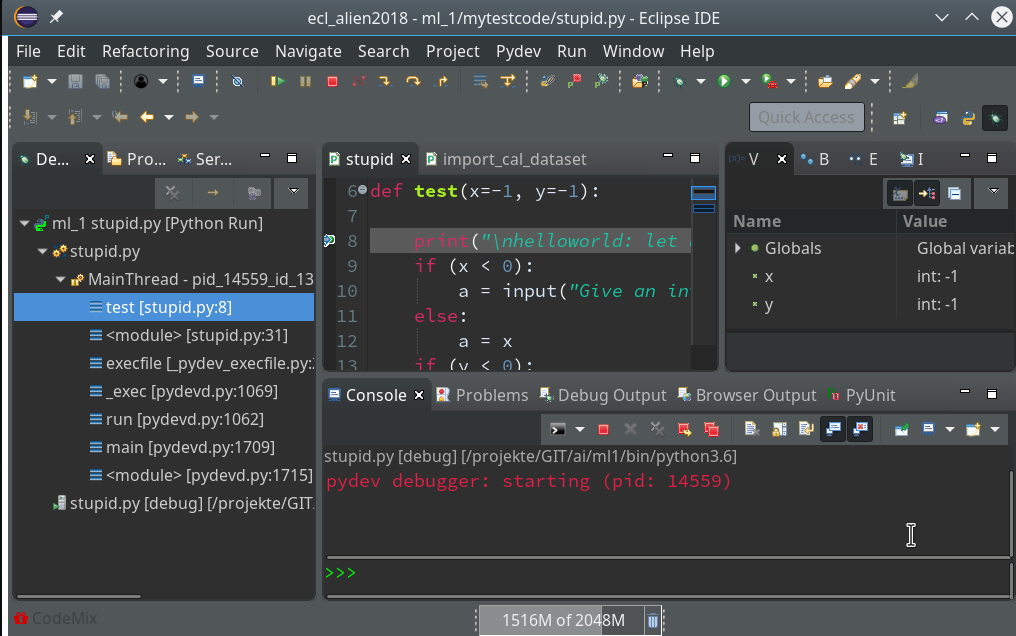
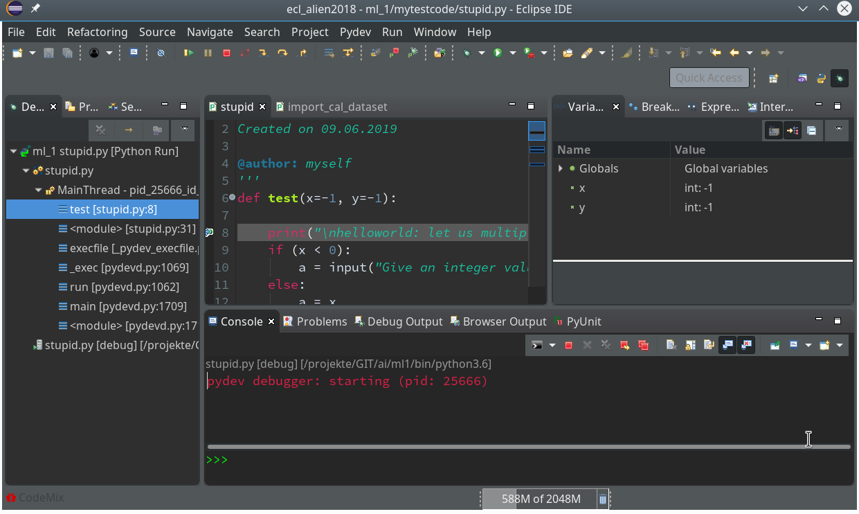
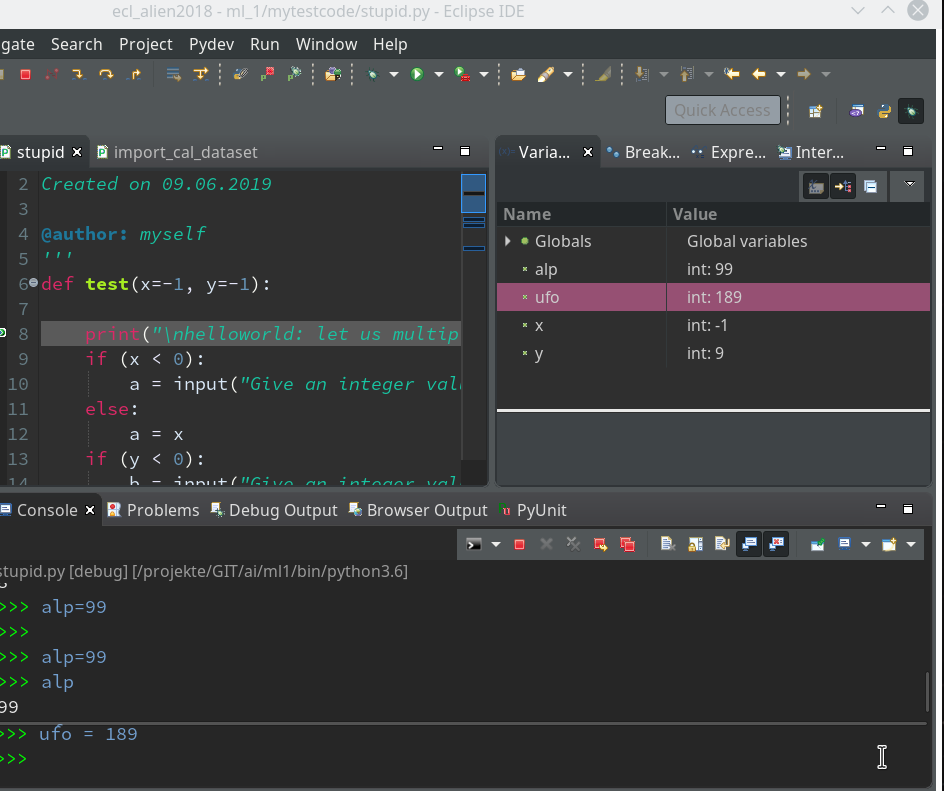
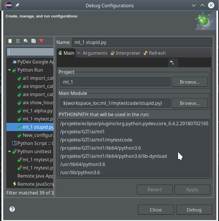
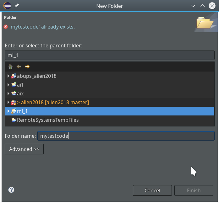
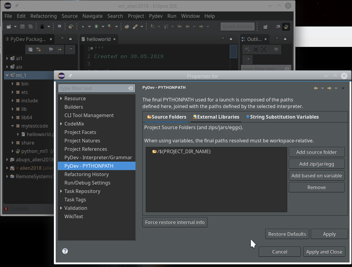
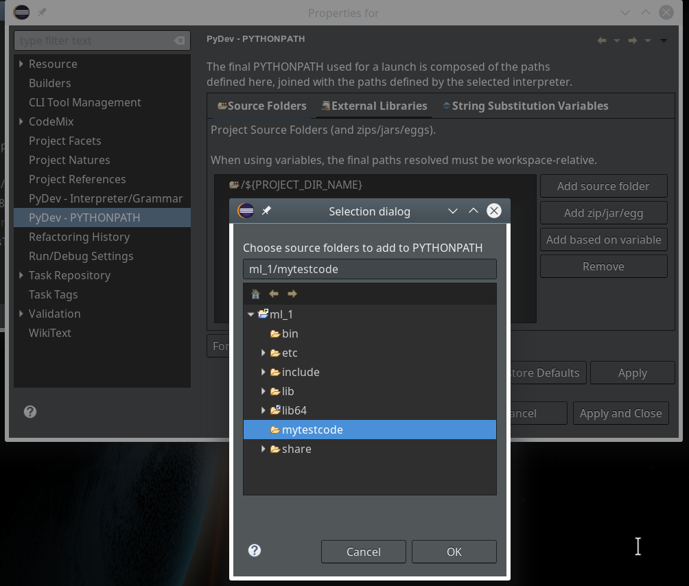
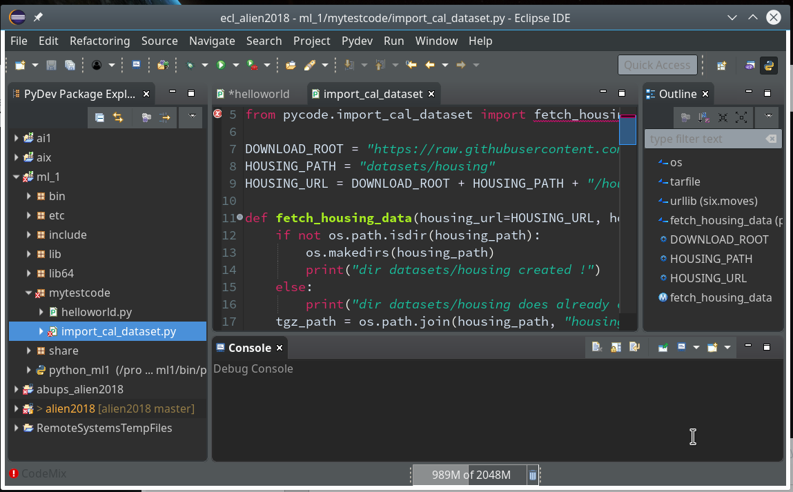
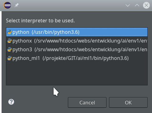
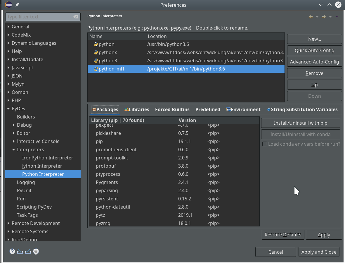
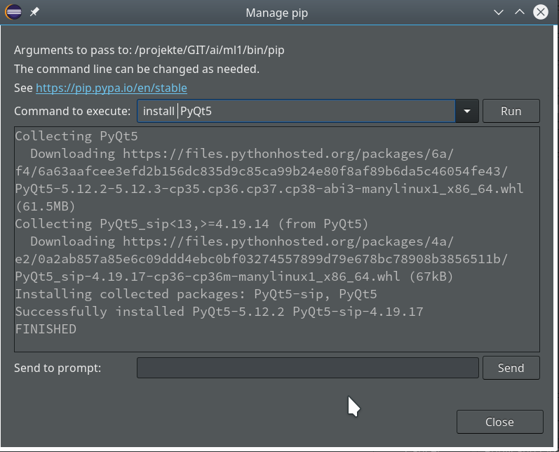
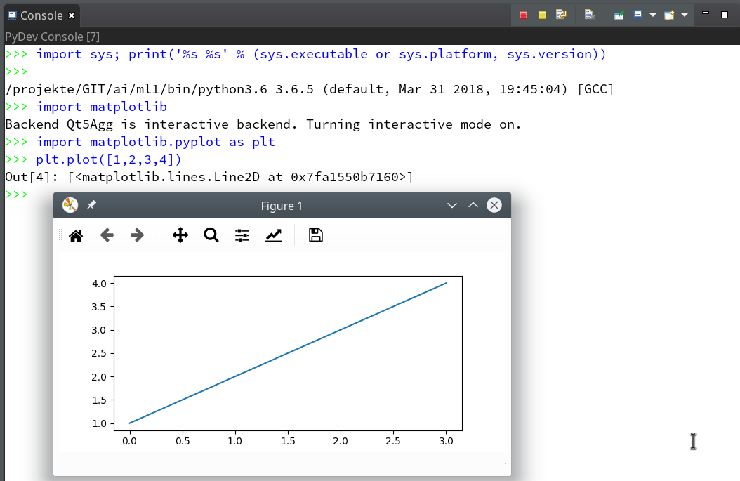
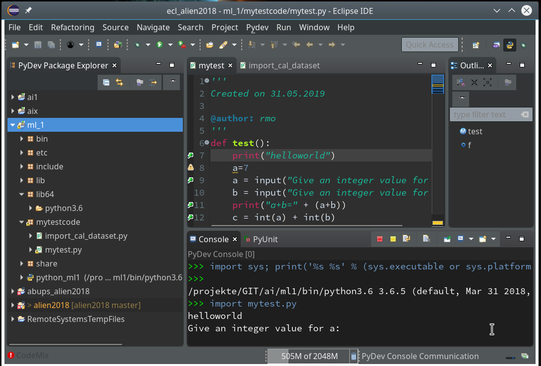
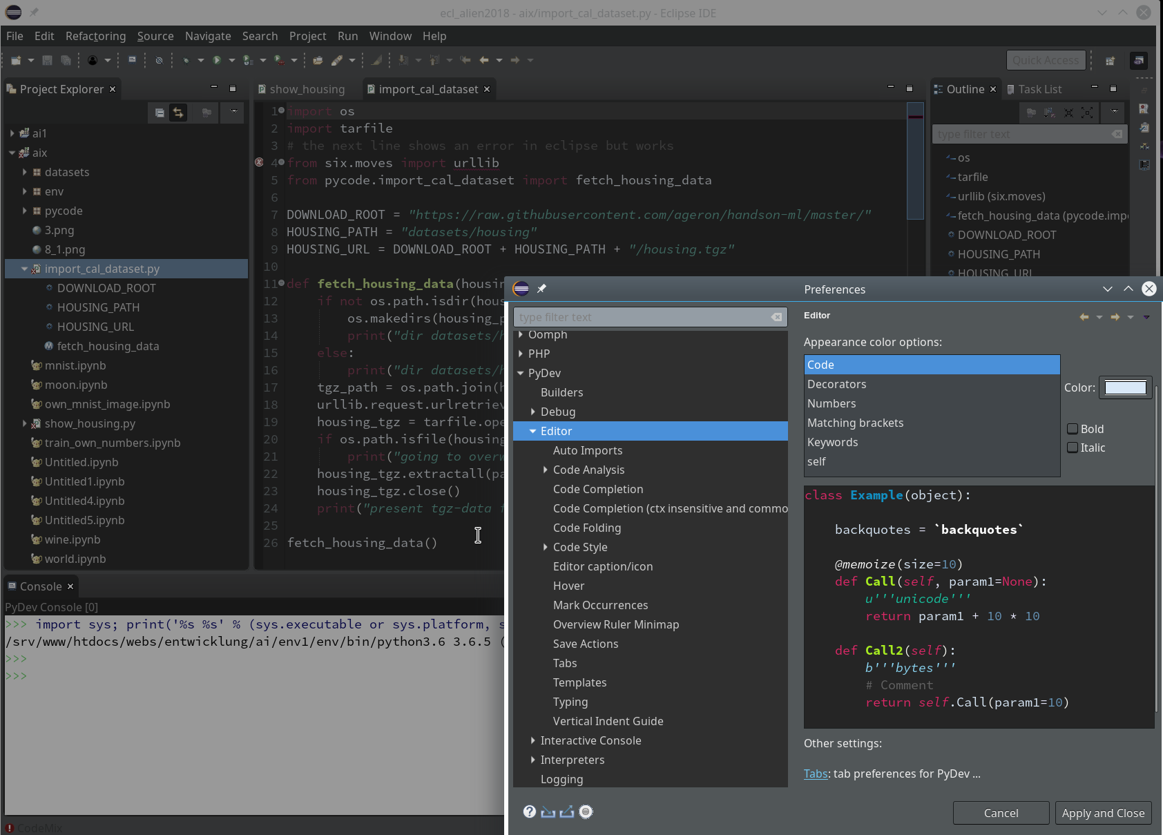
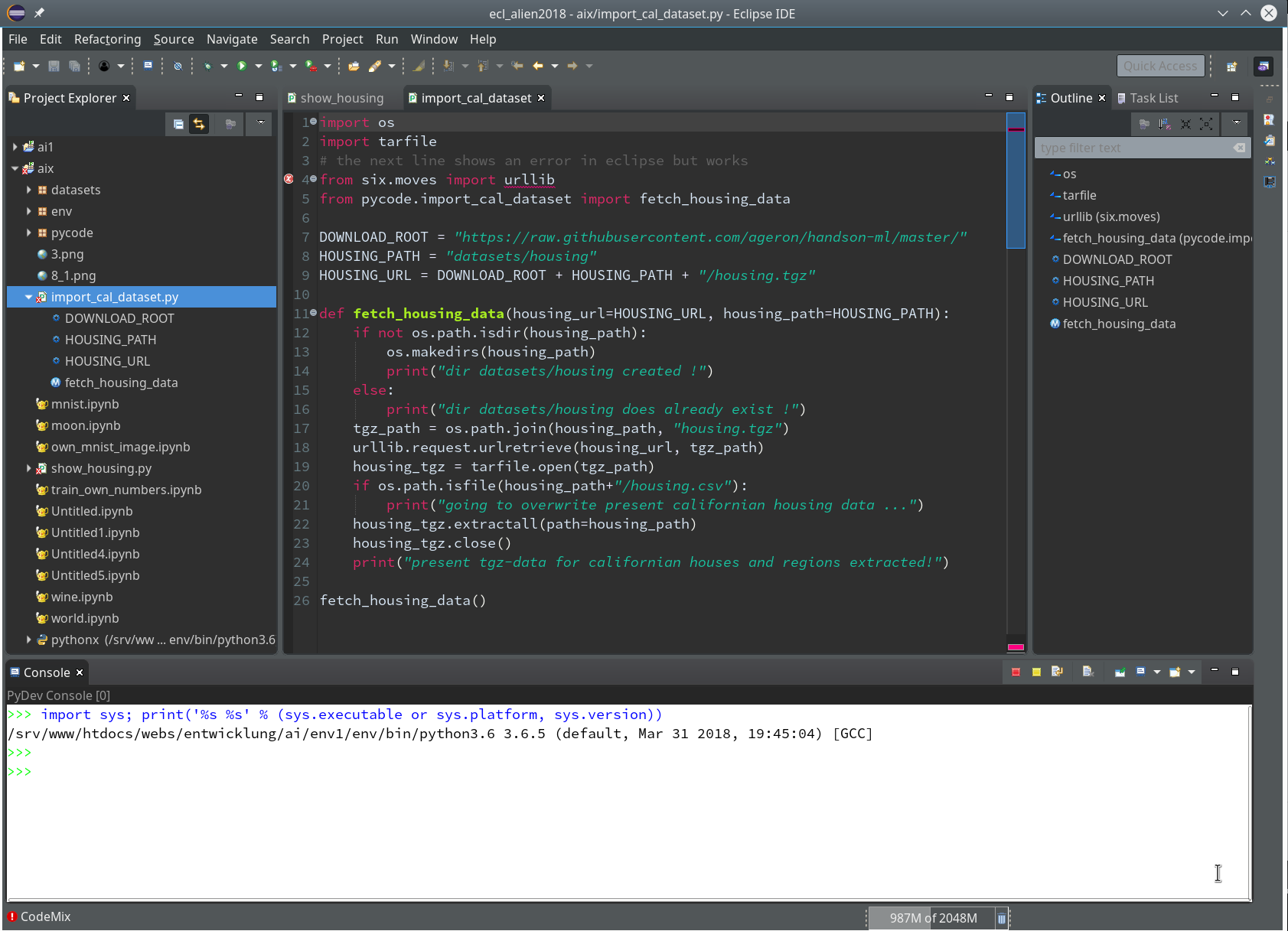
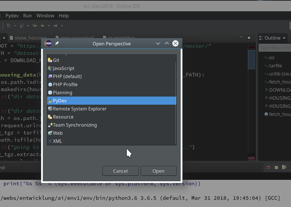
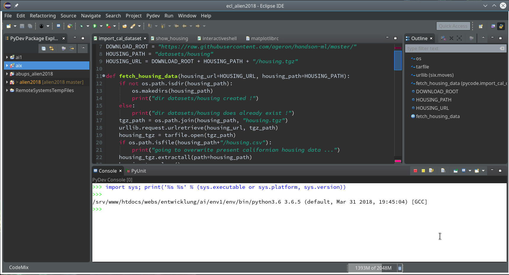
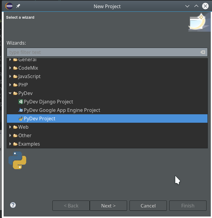
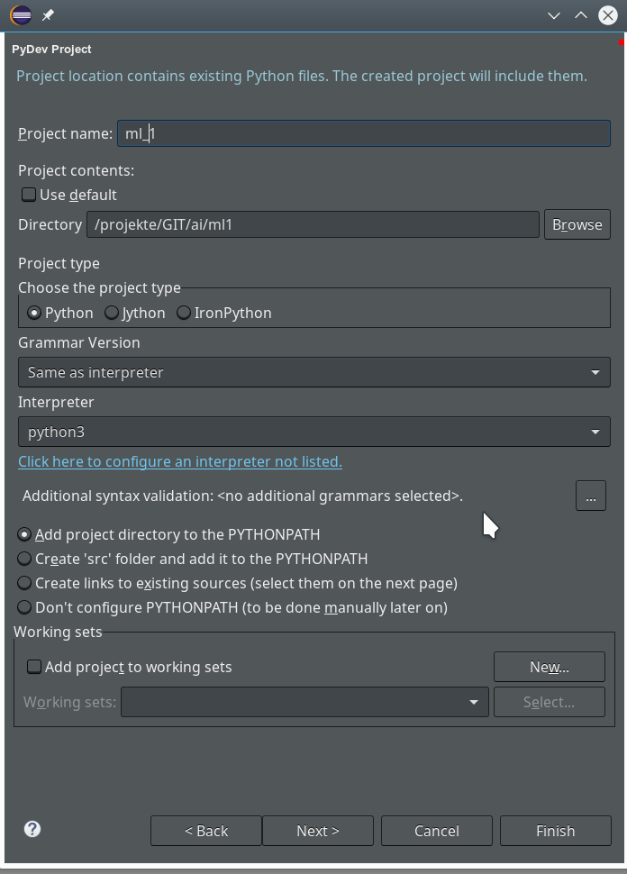
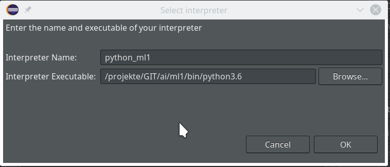
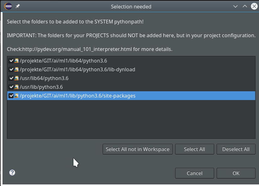
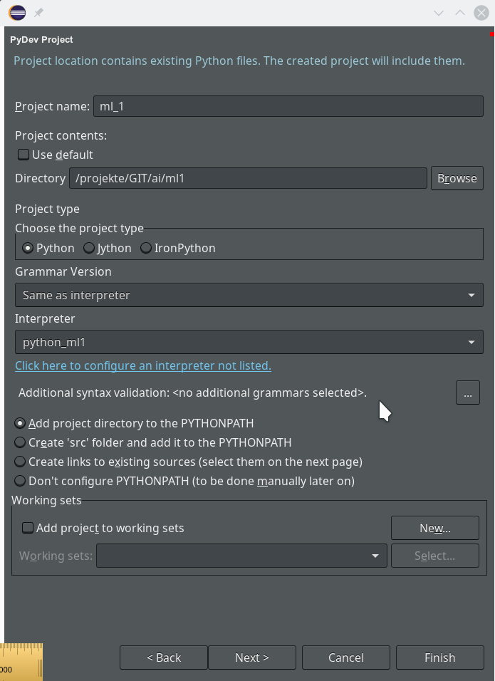
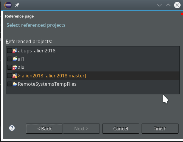
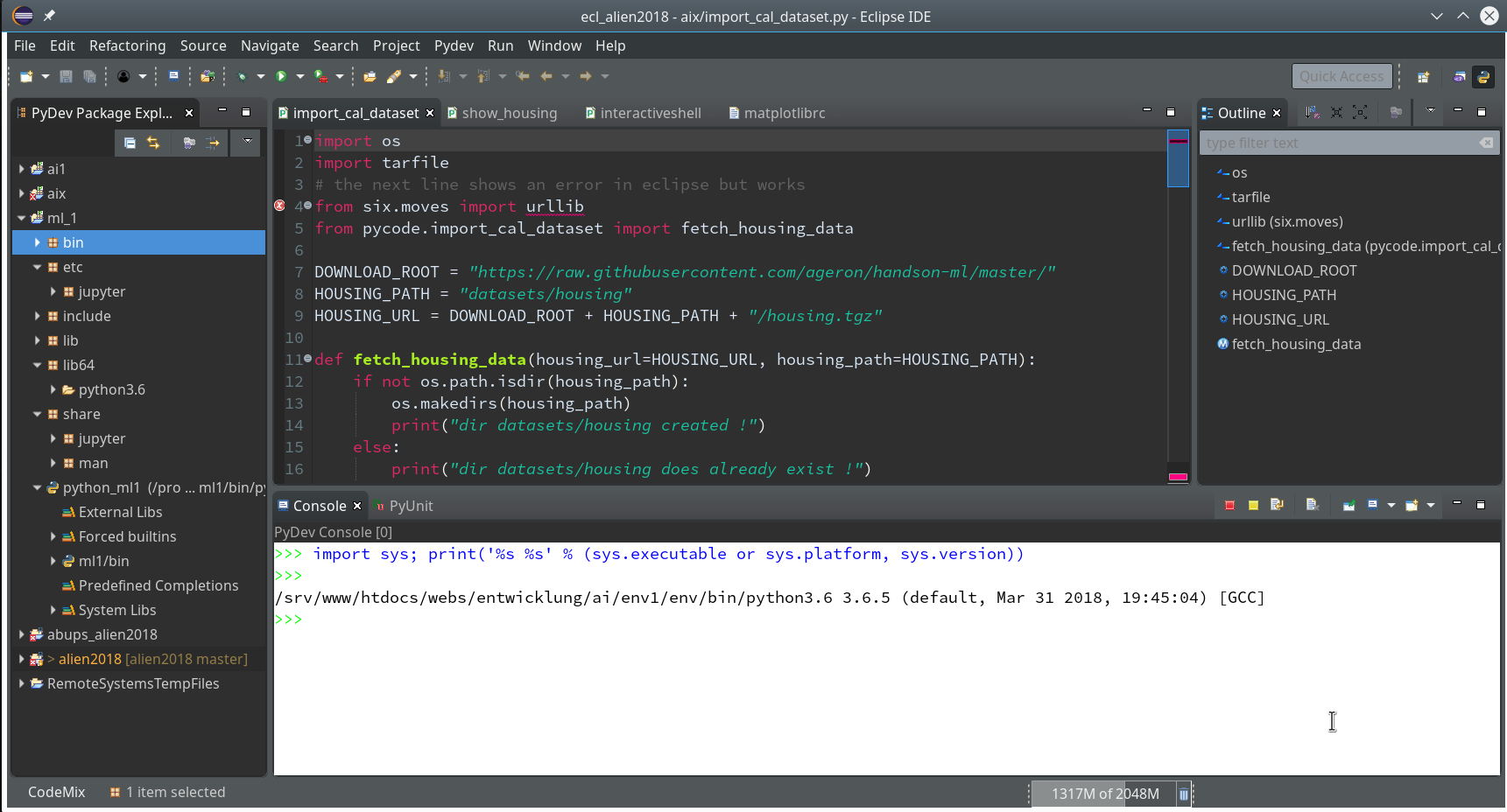
I develop my code as a Python module in an Eclipse/PyDev IDE, which itself uses a virtual Python3 environment. I described the setup of such a development environment in detail in another previous article of this blog. In the resulting directory structure of the PyDev project I place a module “myann.py” at the location “…../ml_1/mynotebooks/mycode/myann.py”. This file shall contain the code of class “MyANN” for our ANN.
Modules and libraries to import
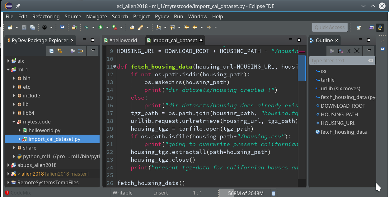
We need to import some libraries at the head of our Python program first:
'''
Module to create a simple layered neural network for the MNIST data set
Created on 23.08.2019
@author: ramoe
'''
import numpy as np
import math
import sys
import time
import tensorflow
from sklearn.datasets import fetch_mldata
from sklearn.datasets import fetch_openml
from keras.datasets import mnist as kmnist
from scipy.special import expit
from matplotlib import pyplot as plt
#from matplotlib.colors import ListedColormap
#import matplotlib.patches as mpat
#from keras.activations import relu
Why do I import “tensorflow” and “keras”?
Well, only for the purpose to create the input data of MNIST quickly. Sklearn’s “fetchml_data” is doomed to end. The alternative “fetch_openml” does not use caching in some older versions and is also in general terribly slow. But, “keras”, which in turn needs tensorflow as a backend, provides its own tool to provide the MNIST data.
We need “scipy” to get an optimized version of the so called “sigmoid“-function – which is an important version of an activation function. We shall use it most of the time. “numpy” and “math” are required for fast array- and math-operations. “time” is required to measure the run time of program segments and “mathplotlib” will help us to visualize some information gathered during and after training.
The “__init__”-function of our class MyANN
We encapsulate most of the required functionality in a class and its methods. Python provides the “__init__”-function, which we can use as a kind of “constructor” – although it technically is not the same as a constructor in other languages. Anyway, we can use it as an interface to feed in parameters and to initialize variables of a class instance.
We shall build up our “__init__()”-function during the next articles step by step. In the beginning we shall only focus on attributes and methods of our class required to import the MNIST data and put them into Numpy arrays and to create the basic network layers.
Parameters
class MyANN:
    def __init__(self,
                 my_data_set = "mnist",
                 n_hidden_layers = 1,
                 ay_nodes_layers = [0, 100, 0], # array which should have as much elements as n_hidden + 2
                 n_nodes_layer_out = 10,  # number of nodes in output layer

                 my_activation_function = "sigmoid",
                 my_out_function        = "sigmoid",

                 vect_mode = 'cols',

                 figs_x1=12.0, figs_x2=8.0,
                 legend_loc='upper right'
                 )
:
        '''
        Initialization of MyANN
        Input:
            data_set: type of dataset; so far only the "mnist", "mnist_784" and the "mnist_keras" datsets are known.
                      We use this information to prepare the input data and learn about the feature dimension.
                      This info is used in preparing the size of the input layer.
            n_hidden_layers = number of hidden layers => between input layer 0 and output layer n
            ay_nodes_layers = [0, 100, 0 ] : We set the number of nodes in input layer_0 and the output_layer to zero
                                             Will be set to real number afterwards by infos from the input dataset.
                                             All other numbers are used for the node numbers of the hidden layers.
            n_nodes_layer_out = expected number of nodes in the output layer (is checked);
                                this number corresponds to the number of categories to be distinguished

            my_activation_function : name of the activation function to use
            my_out_function : name of the "activation" function of the last layer whcih produces the output values

            vect_mode: Are 1-dim data arrays (vectors) ordered by columns or rows ?

            figs_x1=12.0, figs_x2=8.0 : Standard sizing of plots ,
            legend_loc='upper right': Position of legends in the plots

         '''
You see that I defined multiple parameters, which are explained in the Python “doc”-string. We use a “string” to choose the dataset to train our ANN on. To be able to work on other data sets later on we assume that specific methods for importing a variety of special input data sets are implemented in our class. This requires that the class knows exactly which kinds of data sets it is capable to handle. We provide an list with this information below. The other parameters should be clear from their inline documentation.
Initialization of class attributes
We first initialize a bunch of class attributes which we shall use to define the network of layers, nodes, weights, to keep our input data and functions.
        # Array (Python list) of known input data sets
        self.__input_data_sets = ["mnist", "mnist_784", "mnist_keras"]
        self._my_data_set = my_data_set

        # X, y, X_train, y_train, X_test, y_test
            # will be set by analyze_input_data
            # X: Input array (2D) - at present status of MNIST image data, only.
            # y: result (=classification data) [digits represent categories in the case of Mnist]
        self._X       = None
        self._X_train = None
        self._X_test  = None
        self._y       = None
        self._y_train = None
        self._y_test  = None

        # relevant dimensions
        # from input data information;  will be set in handle_input_data()
        self._dim_sets     = 0
        self._dim_features = 0
        self._n_labels     = 0   # number of unique labels - will be extracted from y-data

        # Img sizes
        self._dim_img      = 0 # should be sqrt(dim_features) - we assume square like images
        self._img_h        = 0
        self._img_w        = 0

        # Layers
        # ------
        # number of hidden layers
        self._n_hidden_layers = n_hidden_layers
        # Number of total layers
        self._n_total_layers = 2 + self._n_hidden_layers
        # Nodes for hidden layers
        self._ay_nodes_layers = np.array(ay_nodes_layers)
        # Number of nodes in output layer - will be checked against information from
target arrays
        self._n_nodes_layer_out = n_nodes_layer_out


        # Weights
        # --------
        # empty List for all weight-matrices for all layer-connections
        # Numbering :
        # w[0] contains the weight matrix which connects layer 0 (input layer ) to hidden layer 1
        # w[1] contains the weight matrix which connects layer 1 (input layer ) to (hidden?) layer 2
        self._ay_w = []

        # Known Randomizer methods ( 0: np.random.randint, 1: np.random.uniform )
        # ------------------
        self.__ay_known_randomizers = [0, 1]

        # Types of activation functions and output functions
        # ------------------
        self.__ay_activation_functions = ["sigmoid"] # later also relu
        self.__ay_output_functions     = ["sigmoid"] # later also softmax

        # the following dictionaries will be used for indirect function calls
        self.__d_activation_funcs = {
            'sigmoid': self._sigmoid,
            'relu':    self._relu

            }
        self.__d_output_funcs = {
            'sigmoid': self._sigmoid,
            'softmax': self._softmax
            }

        # The following variables will later be set by _check_and set_activation_and_out_functions()
        self._my_act_func = my_activation_function
        self._my_out_func = my_out_function
        self._act_func = None
        self._out_func = None

        # Plot handling
        # --------------
        # Alternatives to resize plots
        # 1: just resize figure  2: resize plus create subplots() [figure + axes]
        self._plot_resize_alternative = 1
        # Plot-sizing
        self._figs_x1 = figs_x1
        self._figs_x2 = figs_x2
        self._fig = None
        self._ax  = None
                # alternative 2 does resizing and (!) subplots()
        self.initiate_and_resize_plot(self._plot_resize_alternative)

        # ***********
        # operations
        # ***********
        # check and handle input data
        self._handle_input_data()

        print("\nStopping program regularily")
        sys.exit()
To make things not more complicated as necessary I omit the usage of “properties” and a full encapsulation of private attributes. For convenience reasons I use only one underscore for some attributes and functions/methods to allow for external usage. This is helpful in a testing phase. However, many items can in the end be switched to really private properties or methods.
List of known input datasets
The list of known input data sets is kept in the variable “self.__input_data_sets”. The variables
self._X, self._X_train, self._X_test, self._y, self._y_train, self._y_test
will be used to keep all sample data of the chosen dataset – i.e. the training data, the test data for checking of the reliability of the algorithm after training and the corresponding target data (y_…) for classification – in distinct array variables during code execution. The target data in the MNIST case contain the digit a specific sample image ( of _X_train or _X_test..) represents.
All of the named attributes will become Numpy arrays. A method called “_handle_input_data(self)” will load the (MNIST) input data and fill the arrays.
The input arrays “X_…” will via their dimensions provide the information on the number of data sets (_dim_sets) and the number of features (_dim_features). Numpy provides the various dimensions of multidimensional arrays in form of a tuple.
The target data arrays “_y_…” provides the number of “categories” (MNIST: 10 digits) the ANN must distinguish after training. We keep this number in the
attribute “_n_labels”. It is also useful to keep the pixel dimensions of input image data. At least for MNIST we assume quadratic images (_img_h = img_w = _dim_img).
Layers and weights
The number of total layers (“_n_total_layers”) is by 2 bigger than the number of hidden layers (_n_hidden_layers).
We take the number of nodes in the layers from the respective list provided as an input parameter “ay_nodes_layers” to our class. We transform the list into a numpy array “_ay_nodes_layers”. The expected number of nodes in the output layer is used for consistency checks and saved in the variable “_n_nodes_layer_out”.
The “weights” of an ANN must be given in form of matrices: A weight describes a connection between two nodes of different adjacent layers. So we have as many connections as there are node combinations (nodex_(N+1), nodey_N), with “nodex_N” meaning a node on layer L_N and nodey_(N+1) a node on layer L_(N+1).
As the number of layers is not fixed, but can be set by the user, I use a Python list “_ay_w” to collect such matrices in the order of layer_0 (input) to layer_n (output).
Weights, i.e. the matrix elements, must initially be set as random numbers. To provide such numbers we have to use randomizer functions. Depending on the kind (floating point numbers, integer numbers) of random numbers to produce we use at least two randomizers (randint, uniform). For the weights we use the uniform-randomizer.
Allowed activation and output function names are listed in Python dictionaries which point to respective methods. This allows for an “indirect addressing” of these functions later on. You may recognize this by the direct reference of the dictionary elements to defined class methods (no strings are used!).
For the time being we work with the “sigmoid” and the “relu” functions for activation and the “sigmoid” and “softmax” functions for output creation. The attributes “self._act_func” and “self._out_func” are used later on to invoke the functions requested by the respective parameters of the classes interface.
The final part of the code segment given above is used for plot-sizing with the help of “matplotlib”; a method “initiate_and_resize_plot()” takes care of this. It can use 2 alternative ways of doing so.
Read and provide the input data
Now let us turn to some methods. We first need to read in and prepare the input data. We use a method “_handle_input_data()” to work on this problem. For the time being we have only three different ways to load the MNIST dataset from different origins.
    # Method to handle different types of input data sets
    def _handle_input_data(self):
        '''
        Method to deal with the input data:
        - check if we have a known data set ("mnist" so far)
        - reshape as required
        - analyze dimensions and extract the feature dimension(s)
        '''
        # check for known dataset
        try:
            if (self._my_data_set not in self._input_data_sets ):
                raise ValueError
        except ValueError:
            print("The requested input data" + self._my_data_set + " is not known!" )
            sys.exit()


        # handle the mnist original dataset
        if ( self._my_data_set == "mnist"):
            mnist = fetch_mldata('MNIST original')
            self._X, self._y = mnist["data"], mnist["target"]
            print("Input data for dataset " + self._my_data_set + " : \n" + "Original shape of X = " + str(self._X.shape) +
              "\n" + "Original shape of y = " + str(self._y.shape))
            self._X_train, self._X_test, self._y_train, self._y_test = self._X[:60000], self._X[60000:],
 self._y[:60000], self._y[60000:]

        # handle the mnist_784 dataset
        if ( self._my_data_set == "mnist_784"):
            mnist2 = fetch_openml('mnist_784', version=1, cache=True, data_home='~/scikit_learn_data')
            self._X, self._y = mnist2["data"], mnist2["target"]
            print ("data fetched")
            # the target categories are given as strings not integers
            self._y = np.array([int(i) for i in self._y])
            print ("data modified")
            print("Input data for dataset " + self._my_data_set + " : \n" + "Original shape of X = " + str(self._X.shape) +
              "\n" + "Original shape of y = " + str(self._y.shape))
            self._X_train, self._X_test, self._y_train, self._y_test = self._X[:60000], self._X[60000:], self._y[:60000], self._y[60000:]

        # handle the mnist_keras dataset
        if ( self._my_data_set == "mnist_keras"):
            (self._X_train, self._y_train), (self._X_test, self._y_test) = kmnist.load_data()
            len_train =  self._X_train.shape[0]
            #print(len_train)
            print("Input data for dataset " + self._my_data_set + " : \n" + "Original shape of X_train = " + str(self._X_train.shape) +
              "\n" + "Original Shape of y_train = " + str(self._y_train.shape))
            len_test =  self._X_test.shape[0]
            #print(len_test)
            print("Original shape of X_test = " + str(self._X_test.shape) +
              "\n" + "Original Shape of y_test = " + str(self._y_test.shape))
            self._X_train = self._X_train.reshape(len_train, 28*28)
            self._X_test  = self._X_test.reshape(len_test, 28*28)

        # Common Mnist handling
        if ( self._my_data_set == "mnist" or self._my_data_set == "mnist_784" or self._my_data_set == "mnist_keras" ):
            self._common_handling_of_mnist()

        # Other input data sets can not yet be handled
We first check, whether the input parameter fits a known dataset – and raise an error if otherwise. The data come in different forms for the three sources of MNIST. For each set we want to extract the arrays
self._X_train, self._X_test, self._y_train, self._y_test.
We have to do this a bit differently for the 3 cases. Note that the “mnist_784” set from “fetch_openml” gives the target category values in form of strings and not integers. We correct this directly after loading.
The fastest method for importing the MNIST dataset is based on “keras”; the keras function “kmnist.load_data()” provides already a 60000:10000 ratio for training and test data. However, we get the images in a (60000, 28, 28) array shape; we therefore reshape the “_X_train”-array to (60000, 784) and “_X_test”-array to (10000, 784).
Analysis of the input data and the one-hot-encoding of the target labels
A further handling of the MNIST data requires some common analysis.
    # Method for common input data handling of Mnist data sets
    def _common_handling_of_mnist(self):
        print("\nFinal input data for dataset " + self._my_data_set +
              " : \n" + "Shape of X_train = " + str(self._X_train.shape) +
              "\n" + "Shape of y_train = " + str(self._y_train.shape) +
              "\n" + "Shape of X_test = " + str(self._X_test.shape) +
              "\n" + "Shape of y_test = " + str(self._y_test.shape)
              )

        # mixing the training indices
        shuffled_index = np.random.permutation(60000)
        self._X_train, self._y_train = self._X_train[shuffled_index], self._y_train[shuffled_index]

        # set
dimensions
        self._dim_sets = self._y_train.shape[0]
        self._dim_features = self._X_train.shape[1]
        self._dim_img = math.sqrt(self._dim_features)
        # we assume square images
        self._img_h = int(self._dim_img)
        self._img_w = int(self._dim_img)

        # Print dimensions
        print("\nWe have " + str(self._dim_sets) + " data sets for training")
        print("Feature dimension is " + str(self._dim_features) + " (= " + str(self._img_w)+ "x" + str(self._img_h) + ")")

        # we need to encode the digit labels of mnist
        self._get_num_labels()
        self._encode_all_mnist_labels()
As you see we retrieve some of our class attributes which we shall use during training and do some printing. This is trivial. Not as trivial is, however, the handling of the output data:
What shape do we expect for the “_X_train” and “_y_train”? Each element of the input data set is an array with values for all features. Thus the “_X_train.shape” should be (60000, 784). For _y_train we expect a simple integer describing the digit to which the MNIST input image corresponds. Thus we expect a one dimensional array with _y_train.shape = (60000). So far, so good …
But: The output data of our ANN for one input element will be provided as an array of values for our 10 different categories – and not as a simple number. To account for this we need to encode the “_y_train”-data, i.e. the target labels, into an usable array form. We use two methods to achieve this:
    # Method to get the number of target labels
    def _get_num_labels(self):
        self._n_labels = len(np.unique(self._y_train))
        print("The number of labels is " + str(self._n_labels))


    # Method to encode all mnist labels
    def _encode_all_mnist_labels(self, b_print=True):
        '''
        We shall use vectorized input and output - i.e. we process a whole batch of input data sets in parallel
        (see article in the Linux blog)
        The output array will then have the form OUT(i_out_node, idx) where
            i_out_node enumerates the node of the last layer (i.e. the category)
            idx enumerates the data set within a batch,
        After training, if y_train[idx] = 6, we would expect an output value of OUT[6,idx] = 1.0 and OUT[i_node, idx]=0.0 otherwise
        for a categorization decision in the ideal case. Realistically, we will get a distribution of numbers over the nodes
        with values between 0.0 and 1.0 - with hopefully the maximum value at the right node OUT[6,idx].

        The following method creates an arrays OneHot[i_out_node, idx] with
        OneHot[i_node_out, idx] = 1.0, if i_node_out =  int(y[idx])
        OneHot(i_node_out, idx] = 0.0, if i_node_out != int(y[idx])

        This will allow for a vectorized comparison of calculated values and knwon values during training
        '''

        self._ay_onehot = np.zeros((self._n_labels, self._y_train.shape[0]))
        # ay_oneval is just for convenience and printing purposes
        self._ay_oneval = np.zeros((self._n_labels, self._y_train.shape[0], 2))

        if b_print:
            print("\nShape of y_train = " + str(self._y_train.shape))
            print("Shape of ay_onehot = " + str(self._ay_onehot.shape))

        # the next block is just for illustration purposes and a better understanding
        if b_print:
            values = enumerate(self._y_train[0:12])
            print("\nValues of the enumerate structure for the first 12 elements : = ")

            for iv in values:
                print(iv)

        # here we prepare the array for vectorized
comparison
        print("\nLabels for the first 12 datasets:")
        for idx, val in enumerate(self._y_train):
            self._ay_onehot[val, idx ]   = 1.0
            self._ay_oneval[val, idx, 0] = 1.0
            self._ay_oneval[val, idx, 1] = val

        if b_print:
            print("\nShape of ay_onehot = " + str(self._ay_onehot.shape))
            print(self._ay_onehot[:, 0:12])
            #print("Shape of ay_oneval = " + str(self._ay_oneval.shape))
            #print(self._ay_oneval[:, 0:12, :])
The first method only determines the number of labels (= number of categories). We see from the code of the second method that we encode the target labels in the form of two arrays. The relevant one for our optimization algorithm will be “_ay_onehot”. This array is 2-dimensional. Why?
Working with mini-batches
A big advantage of the weight optimization method we shall use later on during training of our MLP is that we will perform weight adjustment for a whole bunch of training samples in one step. Meaning:
We propagate a whole bunch of test data samples in parallel through the grid to get an array with result data (output array) for all samples.
Such a bunch is called a “batch” and if it is significantly smaller than the whole set of training data – a “mini-batch“.
Working with “mini-batches” during the training and learning phase of an ANN is a compromise between
- using the full data set (for gradient evaluation) during each training step (“batch approach“)
- and using just one sample of the training data set for gradient descent and weight corrections (“stochastic approach“).
See chapter 4 of the book of Geron and chapter 2 in the book of Raschka for some thorough information on this topic.
The advantage of mini-batches is that we can use vectorized linear algebra operations over all elements of the batch. Linear Algebra libraries are optimized to perform the resulting vector and matrix operations on modern CPUs and GPUs.
You really should keep the following point in mind to understand the code for the propagation and optimization algorithms discussed in forthcoming articles:
The so called “cost function” will be determined as some peculiar sum over all elements of a batch and the usual evaluation of partial derivatives during gradient descent will be based on matrix operations involving all input elements of a defined batch!
Mini-batches also will help during training in so far as we look at a bunch of multiple selected samples in parallel to achieve bigger steps of our gradient guided descent into an minimum of the cost hyperplane in the beginning – with the disadvantage of making some jumpy stochastic turns on the cost hyperplane instead of a smoother approach.
I probably lost you now 🙂 . The simpler version is: Keep in mind that we later on will work with batches of training data samples in parallel!
However, the separation interface for our categories in the feature space must in the end be adjusted with respect to all given data points of the training set. This means we must perform the training successively for a whole sequence of mini-batches which together cover all available training samples.
What is the shape of the output array?
A single element of the batch is an array of 784 feature values. The corresponding output array is an array with values for 10 categories (here digits). But, what about a whole bunch of test data, i.e. a “batch”?
As I have explained already in my last article
Numpy matrix multiplication for layers of simple feed forward ANNs
the output array for a batch of test data will have the form “_ay_a_Out[i_out_node, idx]” with:
- i_out_node enumerating the node of the last layer, i.e. a possible category
- idx enumerating the data sample within a batch of training data
We shall construct the output function such that it provides something like “probability” values within the interval [0,1] for each node of the output layer. We define a perfectly working MLP as one which – after training – produces a “1.0” at the correct category node (i.e. the expected digit) and “0.0” at all other output nodes.
One-hot-encoding of labels
Later on we must compare the real results for the training samples with the expected correct values. To be able to do this we must build up a 2-dim array of the same shape as “_ay_a_out” with correct output values for all test samples of the batch. E.g.: If we expect the digit 7 for the input array of a sample with index idx within the set of training data, we need a 2-dim output array with the element [[0,0,0,0,0,0,0,1,0,0], idx]. The derivation of such an array from a given category label is called “one-hot-encoding“.
By using Numpy’s zero()-function and Pythons “enumerate()”-function we can achieve such an encoding for all data elements of the training data set. See the method “_encode_all_mnist_labels()”. Thus, the array “_ay_onehot” will have a shape of (10, 60000). From this 2-dim array we can later slice out bunches of consecutive test data for mini-batches. The array “_ay_oneval” is provided for convenience and print purposes, only: it provides the expected digit value in addition.
First tests via a Jupyter notebook
Let us test the import of the input data and the label encoding with a Jupyter notebook. In previous articles I have described already how to use such a notebook. I set up a Jupyter notebook called “myANN” (in my present working directory “/projekte/GIT/ai/ml1/mynotebooks”).

I start it with
myself@mytux:/projekte/GIT/ai/ml1> source bin/activate
(ml1) myself@mytux:/projekte/GIT/ai/ml1> jupyter notebook
[I 15:07:30.953 NotebookApp] Writing notebook server cookie secret to /run/user/21001/jupyter/notebook_cookie_secret
[I 15:07:38.754 NotebookApp] jupyter_tensorboard extension loaded.
[I 15:07:38.754 NotebookApp] Serving notebooks from local directory: /projekte/GIT/ai/ml1
[I 15:07:38.754 NotebookApp] The Jupyter Notebook is running at:
[I 15:07:38.754 NotebookApp] http://localhost:8888/?token=06c2626c8724f65d1e3c4a50457da0d6db414f88a40c7baf
[I 15:07:38.755 NotebookApp] Use Control-C to stop this server and shut down all kernels (twice to skip confirmation).
[C 15:07:38.771 NotebookApp]
and add two cells. The first one is for the import of libraries.
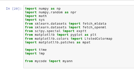
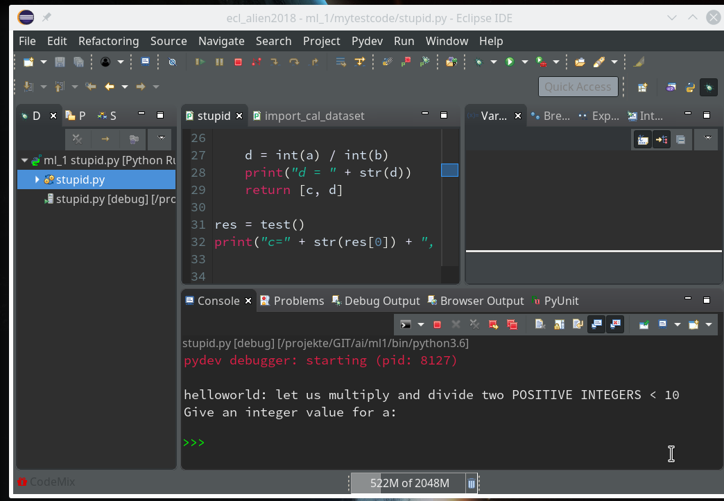
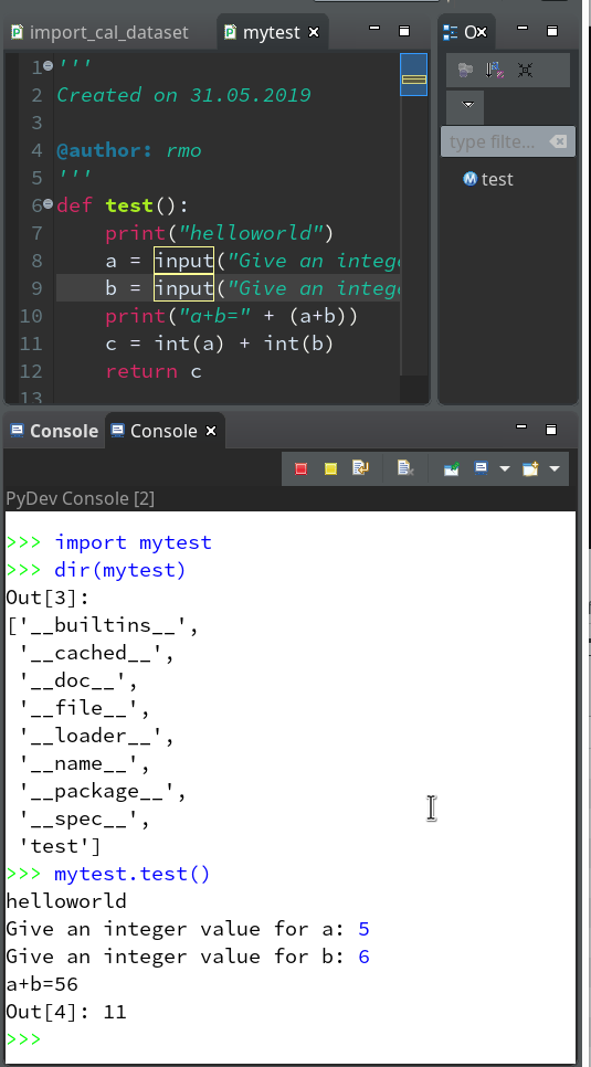
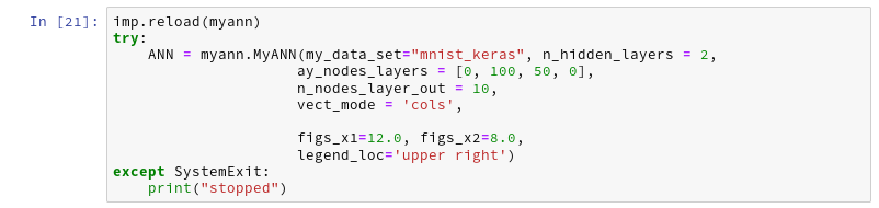
By the last line I import my present class code. With the second cell I create an instance of my class; the “__init__()”-function is automatically executed ad calls the other methods defined so far:
The output is:
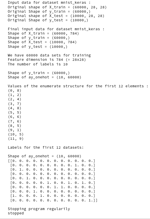
Note that the display of “_ay_onehot” shows the categories in vertical (!) direction (rows) and the index for the input data element in horizontal direction (columns)! You see that the labels in the enumerate structure correspond to the “1”s in the “_ay_onehot”-array.
Conclusion
Importing the MNIST dataset into Numpy arrays via Keras is simple – and has a good performance. We have learned a bit about “one-hot-encoding” and prepared an array “_ay_onehot”, which we shall use during ANN training and weight optimization. It will allow us to calculate a difference between the actual output values of the ANN at the nodes of the output layer and a “1.0” value at the node for the expected sample category and “0.0” otherwise.
In the next article
A simple program for an ANN to cover the Mnist dataset – II
we shall define initial weights for our ANN.
Literature and links
Referenced Books
“Python machine Learning”, Seb. Raschka, 2016, Packt Publishing, Birmingham, UK
“Machine Learning mit Sckit-Learn & TensorFlow”, A. Geron, 2018, O’REILLY, dpunkt.verlag GmbH, Heidelberg, Deutschland
Links regarding cost (or loss) functions and logistic regression
https://towardsdatascience.com/introduction-to-logistic-regression-66248243c148
https://cmci.colorado.edu/classes/INFO-4604/files/slides-5_logistic.pdf
Wikipedia article on Loss functions for classification
https://towardsdatascience.com/optimization-loss-function-under-the-hood-part-ii-d20a239cde11
https://stackoverflow.com/questions/32986123/why-the-cost-function-of-logistic-regression-has-a-logarithmic-expression
https://medium.com/technology-nineleaps/logistic-regression-gradient-descent-optimization-part-1-ed320325a67e
https://blog.algorithmia.com/introduction-to-loss-functions/
uni leipzig on logistic regression
Further articles in this series
A simple Python program for an ANN to cover the MNIST dataset – XIV – cluster detection in feature space
A simple Python program for an ANN to cover the MNIST dataset – XIII – the impact of regularization
A simple Python program for an ANN to cover the MNIST dataset – XII – accuracy evolution, learning
rate, normalization
A simple Python program for an ANN to cover the MNIST dataset – XI – confusion matrix
A simple Python program for an ANN to cover the MNIST dataset – X – mini-batch-shuffling and some more tests
A simple Python program for an ANN to cover the MNIST dataset – IX – First Tests
A simple Python program for an ANN to cover the MNIST dataset – VIII – coding Error Backward Propagation
A simple Python program for an ANN to cover the MNIST dataset – VII – EBP related topics and obstacles
A simple Python program for an ANN to cover the MNIST dataset – VI – the math behind the „error back-propagation“
A simple Python program for an ANN to cover the MNIST dataset – V – coding the loss function
A simple Python program for an ANN to cover the MNIST dataset – IV – the concept of a cost or loss function
A simple Python program for an ANN to cover the MNIST dataset – III – forward propagation
A simple Python program for an ANN to cover the MNIST dataset – II – initial random weight values