
Last week I tried to perform some systematic calculations with a “Variational Autoencoder” [VAE] for a presentation about Machine Learning [ML]. I wanted to apply VAEs to different standard datasets (MNIST Fashion, CIFAR 10, Celebrity) and demonstrate some basic capacities of VAE algorithms. A standard task … well covered by several introductory books on ML.
Actually, I had some 2 years old Python modules for VAEs available – all based on recommendations in the literature. My VAE-model setup had been done with Keras. Moreprecisely the version integrated into Tensorflow 2 [TF2]. But I ran into severe trouble with my present Tensorflow versions, namely 2.7 and 2.8. The cause of the problems was my handling of the so called Kullback-Leibler [KL] loss in combination with the “eager execution mode” of TF2.
Actually, the problems may already have arisen with earlier TF versions. With this post series I hope to save time for some readers who, as myself, are no ML professionals. In a first post I will briefly repeat some basics about Autoencoders [AEs] and Variational Autoencoders [VAEs]. In a second post we shall build a simple Autoencoder. In a third post I shall turn to VAEs and discuss some variants for dealing with the KL loss – all variants will be picked from recipes of ML teaching books. I shall demonstrate afterward that some of these recipes fail for TF 2.8. A fourth post will discuss the problem with “eager execution” and derive a practical rule for calculations based on layer specific data. In three further posts I apply the rule in the form of three different variants for the KL loss of VAE models. I will set up the VAE models with the help of the functional Keras API. The suggested solutions all do work with Tensorflow 2.7 and 2.8.
If you are not interested in the failures of classical approaches to the KL loss presented in teaching books on ML and if you are not at all interested in theory you may skip the first four posts – and jump to the solutions.
Some basics of VAEs – a brief introduction
I assume that the reader is already familiar with the concepts of “Variational Autoencoders”. I nevertheless discuss some elements below to get a common vocabulary.
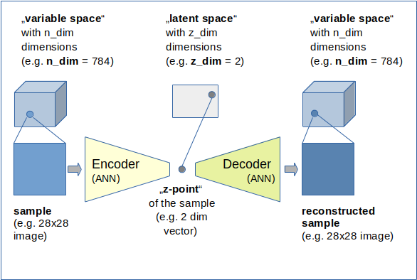
I call the vector space which describes the input samples the "variable space". As AEs and VAEs are typically used for images this “variable space” has many dimensions – from several hundred up to millions. I call the number of these dimensions "n_dim".
An input sample can either be represented as a vector in the variable space or by a multi-ranked tensor. An image with 28×28 pixels and gray “colors” corresponds to a 784 dimensional vector in the variable space or a a “rank 2 tensor” with the shape (28, 28). I use the term “rank” to avoid any notional ambiguities regarding the term “dimensions”. Remember that people sometimes speak of 2-“dimensional” Numpy matrices with 28 elements in each dimension.
An Autoencoder [AE] typically consists of two connected artificial neural networks [ANN]:
- Encoder : maps a point of the “variable space” to a point in the so called “latent space”
- Decoder : maps a point of the “latent space” to a point in the “variable space”.
Both parts of an AE can e.g. be realized with Dense and/or Conv2D layers. See the next post for a simple example of a VAE layer-layout. With Keras both ANNs can be defined as individual “Keras models” which we later connect.
Some more details:
- Encoder:
The Encoder ANN creates a vector for each input sample (mostly images) in a low-dimensional vector space, often called the “latent space“. I will sometimes use the abbreviation “z-space” for it and call a point in it a “z-point“. The dimensions of the “z-space” are given by a number “z_dim“. A “z-point” is therefore represented as a z-dimensional vector (a special kind of a tensor of rank 1). The Encoder realizes a non-linear transformation of n-dimensional vectors to z-dimensional vectors. Encoders, actually, are very effective data compressors. z_dim may take numbers between 2 and a few hundred – depending on the complexity of data and objects represented by the input samples with much higher dimensions (some hundreds to millions). - Decoder:
The “Decoder” ANN instead takes arbitrary low dimensional vectors from the “latent space” as input and creates or better “reconstructs” tensors with the same rank and dimensions as the input samples. These output samples can, of course, also be represented by n-dimensional vectors in the original variable space. The Decoder is a kind of inversion of the “Encoder”. This is also reflected in its structure as we shall see later on. One objective of (V)AEs is that the reconstruction vector for a defined input sample should be pretty close to the input vector of the very same sample – with some metric to measure distances. In natural terms for images: An output image of a Decoder should be pretty comparable to the input image of the Encoder, when we feed the Decode with the z-dim vector created by the Encoder.
A Keras model for the (V)AE can be build by connecting the models for the Encoder and Decoder. The (V)AE model is trained as a whole to minimize differences between the input (e.g. an image) presented to the Encoder and the created output of the Decoder (a reconstructed image). A (V)AE is trained “unsupervised” in the sense that the “label data” for the training are identical to the encoder input samples.
Encoder and Decoder as CNNs?
When you build the Encoder and the Decoder as a “Convolutional Neutral Networks” [CNNs] they support data compression and reconstruction very effectively by a parallel extraction of basic “features” of the input samples and putting the related information into neural “maps”. (The neurons in such a “map” react sensitively to correlation patterns of components of the tensors representing the input data samples.) For images such CNN networks would accept rank 2 tensors.
Note that the (V)AE’s knowledge about basic “features” (or data correlations) in the input samples is encoded in the weights of the “Encoder” and “Decoder”. The points in the “latent space” which represent the input samples may show cluster patterns. The clusters could e.g. be used in classification tasks. However, without an appropriate Decoder with fitted weights you will not be able to reconstruct a complete image from a point in the z-space. Similar to encryption scenarios the Decoder is a kind of “key” to retrieve original information (even with reduced detail quality).
Variational Autoencoders
Variational Autoencoders take care about a reasonable data organization in the latent space – in addition to data compression. The objective is to get well defined and segregated clusters there for “features” or maybe even classes of input samples. But the clusters should also be confined in a common, relatively small and compact region of the z-space.
To achieve this goal one judges the arrangement of data points, i.e. their distribution in the latent space, with the help of a special loss contribution. I.e. we use specially designed costs which punish vast extensions of the data distribution off the origin in the latent space.
The data distribution is controlled by parameters, typically a mean value “mu” and a standard deviation or variance “var”. These parameters provide additional degrees of freedom during training. The special loss used to control the predicted distribution in comparison to an ideal one is the so called “Kullback-Leibler” [KL] loss. It measures the “distance” of the real data distribution in the latent space from a more confined ideal one.
You find more information about the KL-loss in the books of D. Foster and R. Atienza named in the last section of this post.
Why the fuss about VAEs and the KL-loss at all?
Why are VAEs and their “KL loss” important? Basically, because VAEs help you to confine data in the z-space. Especially when the latent space has a very low number of dimensions. VAEs thereby also help to condense clusters which may be dominated by samples of a specific class or a label for some specific feature. Thus VAEs provide the option to define paths between such clusters and allow for “feature arithmetics” via vector operations.
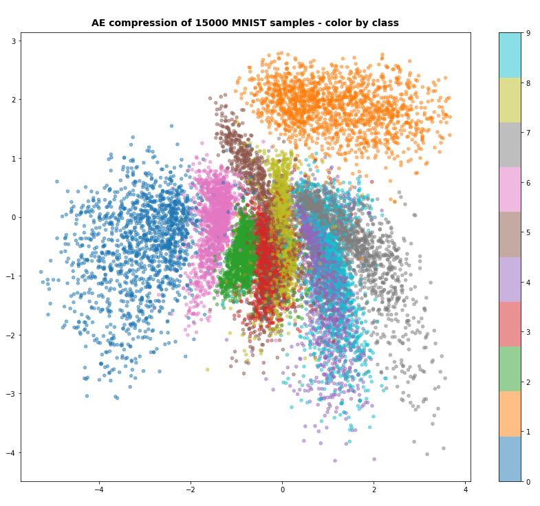
See the following images of MNIST data mapped into a 2-dimensional latent space by a standard Autoencoder:

Despite the fact that the AE’s sub-nets (CNNs) already deal very well with with features the resulting clusters for the digit classes are spread in a relatively large area of the latent space: [-7 ≤ x ≤ +7], [6 ≥ y ≥ -9]. Had we used dense layers of a MLP only, the spread of data points would have covered an even bigger area in the latent space.
The following three plots resulted from VAEs with different parameters. Watch the scale of the axes.

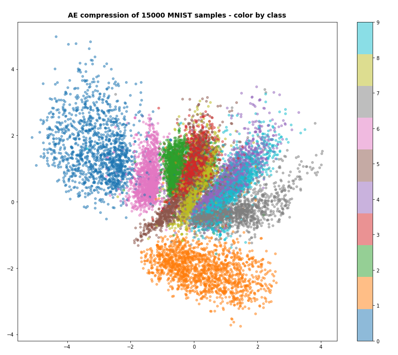
The data are now confined to a region of around [[-4,4], [-4,4]] with respect to [x,y]-coordinates in the “latent space”. The available space is more efficiently used. So, you want to avoid any problems with the KL-loss in VAEs due to some peculiar requirements of Tensorflow 2.x.
Conclusion
AEs are easy to understand, VAEs have subtle additional properties which seem to be valuable for certain tasks. But also for principle reasons we want to enable a Keras model of an ANN to calculate quantities which depend on the elements of one or a few given layers. One example of such a quantity is the KL loss.
In the next post
Variational Autoencoder with Tensorflow 2.8 – II – an Autoencoder with binary-crossentropy loss
we shall build an Autoencoder and apply it to the MNIST dataset. This will give us a reference point for VAEs later.
Stay tuned ….
Ceterum censeo: The worst living fascist and war criminal today, who must be isolated, denazified and imprisoned, is the Putler.
Further articles in this series
Variational Autoencoder with Tensorflow – II – an Autoencoder with binary-crossentropy loss
Variational Autoencoder with Tensorflow – III – problems with the KL loss and eager execution
Variational Autoencoder with Tensorflow – IV – simple rules to avoid problems with eager execution
Variational Autoencoder with Tensorflow – V – a customized Encoder layer for the KL loss
Variational Autoencoder with Tensorflow – VI – KL loss via tensor transfer and multiple output
Variational Autoencoder with Tensorflow – VII – KL loss via model.add_loss()
Variational Autoencoder with Tensorflow – VIII – TF 2 GradientTape(), KL loss and metrics
Variational Autoencoder with Tensorflow – IX – taming Celeb A by resizing the images and using a generator
Variational Autoencoder with Tensorflow – X – VAE application to CelebA images
Variational Autoencoder with Tensorflow – XI – image creation by a VAE trained on CelebA
Variational Autoencoder with Tensorflow – XII – save some VRAM by an extra Dense layer in the Encoder
Variational Autoencoder with Tensorflow – XIII – Does a VAE with tiny KL-loss behave like an AE? And if so, why?