Variational Autoencoder with Tensorflow – VII – KL loss via model.add_loss()

I continue my series on options regarding the treatment of the Kullback-Leibler divergence as a loss [KL loss] in Variational Autoencoder [VAE] setups.

Variational Autoencoder with Tensorflow – I – some basics
Variational Autoencoder with Tensorflow – II – an Autoencoder with binary-crossentropy loss
Variational Autoencoder with Tensorflow – III – problems with the KL loss and eager execution
Variational Autoencoder with Tensorflow – IV – simple rules to avoid problems with eager execution
Variational Autoencoder with Tensorflow – V – a customized Encoder layer for the KL loss
Variational Autoencoder with Tensorflow – VI – KL loss via tensor transfer and multiple output

Our objective is to find solutions which avoid potential problems with the eager execution mode of present Tensorflow 2 implementations. Popular recipes of some teaching books on ML may lead to non-working codes in present TF2 environments. We have already looked at two working alternatives.

In the last post we transferred the “mu” and “log_var” tensors from the Encoder to the Decoder and fed some Keras standard loss functions with these tensors. These functions could in turn be inserted into the model.compile() statement. The approach was a bit complex because it involved multi-input-output model definitions for the Encoder and Decoder.

The present article will discuss a third and lighter approach – namely using the Keras add_loss() mechanism on the level of a Keras model, i.e. model.add_loss().

The advantage of this function is that its parameter interface is not reduced to the form of standardized Keras cost function interfaces which I used in my last post. This gives us flexibility. A solution based on model.add_loss() is also easy to understand and realize on the programming level. It is, however, an approach which may under certain conditions reduce performance by roughly a factor between 1.3 and 1.5 – which is significant. I admit that I have not yet understood what the reasons are. But the concrete solution version I present below works well.

The strategy

The way how to use Keras’ add_loss() functionality is described in the Keras documentation. I quote from this part of TF2’s documentation about the use of add_loss():

This method can also be called directly on a Functional Model during construction. In this case, any loss Tensors passed to this Model must be symbolic and be able to be traced back to the model’s Inputs. These losses become part of the model’s topology and are tracked in get_config.

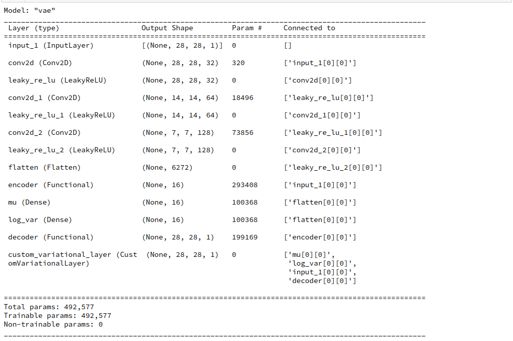
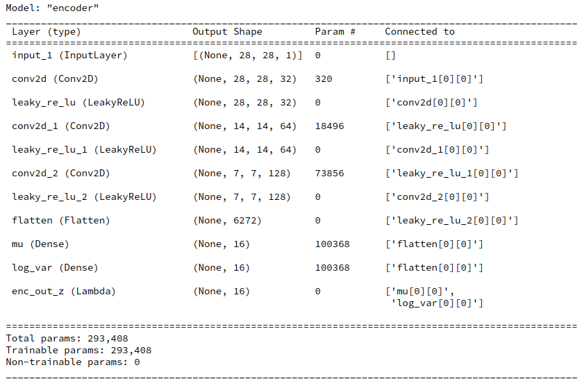
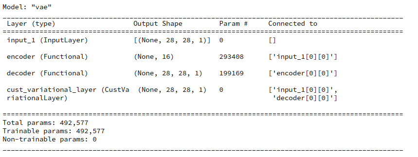
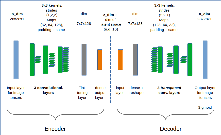
The documentation also contains a simple example. The strategy is to first define a full VAE model with standard mu and log_var layers in the Encoder part – and afterwards add the KL-loss to this model. This is depicted in the following graphics:

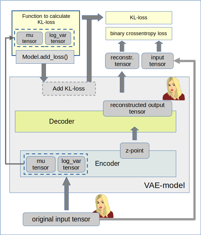
We implement this strategy below via the Python class for a VAE setup which we have used already in the last 4 posts of this series. We control the Keras model setup and the layer construction by the parameter “solution_type”, which I have introduced in my last post.

Cosmetic changes to the Encoder/Decoder parts and the model creation

The class method _build_enc(self, …) can remain as it was defined in the last post. We just have to change the condition for the layer setup as follows:

Change to _build_enc(self, …)

... # see other posts 
...
        # The Encoder Model 
        # ~~~~~~~~~~~~~~~~~~~
        # With extra KL layer or with vae.add_loss()
        if solution_type == 0 or solution_type == 2: 
            self.encoder = Model(self._encoder_input, self._encoder_output)
        
        # Transfer solution => Multiple outputs 
        if solution_type == 1: 
            self.encoder = Model(inputs=self._encoder_input, outputs=[self._encoder_output, self.mu, self.log_var], name="encoder")

Something similar holds for the Decoder part _build_decoder(…):

Change to _build_dec(self, …)

... # see other posts 
...
        # The Decoder model 
        # solution_type == 0/2: Just the decoded input 
        if self.solution_type == 0 or self.solution_type == 2: 
            self.decoder = Model(self._decoder_inp_z, self._decoder_output)
        
        # solution_type == 1: The decoded tensor plus the transferred tensors mu and log_var a for the variational distribution 
        if self.solution_type == 1: 
            self.decoder = Model([self._decoder_inp_z, self._dec_inp_mu, self._dec_inp_var_log], 
                                 [self._decoder_output, self._dec_mu, self._dec_var_log], name="decoder")

A similar change is done regarding the model definition in the method _build_VAE(self):

Change to _build_VAE(self)

        solution_type = self.solution_type
        
        if solution_type == 0 or solution_type == 2:
            model_input  = self._encoder_input
            model_output = self.decoder(self._encoder_output)
            self.model = Model(model_input, model_output, name="vae")

... # see other posts 
...


Changes to the method compile_myVAE(self, learning_rate)

More interesting is a function which we add inside the method compile_myVAE(self, learning_rate, …).

Changes to compile_myVAE(self, learning_rate):

    # Function to compile the full VAE
    # ~~~~~~~~~~~~~~~~~~~~~~~~~~~~~~~~~~~~~~~~~~~~~ 
    def compile_myVAE(self, learning_rate):

        # Optimizer
        # ~~~~~~~~~ 
        optimizer = Adam(learning_rate=learning_rate)
        # save the learning rate for possible intermediate output to files 
        self.learning_rate = learning_rate
        
        # Parameter "fact" will be used by the cost functions defined below to scale the KL loss relative to the BCE loss 
        fact = self.fact
        
        # Function for solution_type == 1
        # ~~~~~~~~~~~~~~~~~~~~~~~~~~~~~~~~~  
        @tf.function
        def mu_loss(y_true, y_pred):
            loss_mux = fact * tf.reduce_mean(tf.square(y_pred))
            return loss_mux
        
        @tf.function
        def logvar_loss(y_true, y_pred):
            loss_varx = -fact * tf.reduce_mean(1 + y_pred - tf.exp(y_pred))    
            return loss_varx

        # Function for solution_type == 2 
        # ~~~~~~~~~~~~~~~~~~~~~~~~~~~~~~~~
        # We follow an approach described at  
        # https://www.tensorflow.org/api_docs/python/tf/keras/layers/Layer
        # NOTE: We can NOT use @tf.function here 
        def get_kl_loss(mu, log_var):
            kl_loss = -fact * tf.reduce_mean(1 + log_var - tf.square(mu) - tf.exp(log_var))
            return kl_loss

        # Required operations for solution_type==2 => model.add_loss()
        # ~~~~~~~~~~~~~~~~~~~~~~~~~~~~~~~~~~~~~~~~~
        res_kl = get_kl_loss(mu=self.mu, log_var=self.log_var)
        if self.solution_type == 2: 
            self.model.add_loss(res_kl)    
            self.model.add_metric(res_kl, name='kl', aggregation='mean')
        
        # Model compilation 
        # ~~~~~~~~~~~~~~~~~~~~
        if self.solution_type == 0 or self.solution_type == 2: 
            self.model.compile(optimizer=optimizer, loss="binary_crossentropy",
                               metrics=[tf.keras.metrics.BinaryCrossentropy(name='bce')])
        
        if self.solution_type == 1: 
            self.model.compile(optimizer=optimizer
                               , loss={'vae_out_main':'binary_crossentropy', 'vae_out_mu':mu_loss, 'vae_out_var':logvar_loss} 
                               #, metrics={'vae_out_main':tf.keras.metrics.BinaryCrossentropy(name='bce'), 'vae_out_mu':mu_loss, 'vae_out_var': logvar_loss }
                               )

I have supplemented function get_kl_loss(mu, log_var). We explicitly provide the tensors “self.mu” and “self.log_var” via the function’s interface and thus follow one of our basic rules for the Keras add_loss()-functionality (see post IV).
Note that this is a MUST to get a working solution for eager execution mode!

Interestingly, the flexibility of model.add_loss() has a price, too. We can NOT use a @tf.function indicator here – in contrast to the standard cost functions which we used in the last post.

Note also that I have added some metrics to get detailed information about the size of the crossentropy-loss and the KL-loss during training!

Cosmetic change to the method for training

Eventually we must include solution_type==2 in method train_myVAE(self, x_train, batch_size, …)

Changes to train_myVAE(self, x_train, batch_size,…)

... # see other posts 
...
        if self.solution_type == 0 or self.solution_type == 2: 
            self.model.fit(     
                x_train
                , x_train
                , batch_size = batch_size
                , shuffle = True
                , epochs = epochs
                , initial_epoch = initial_epoch
            )
        
        if self.solution_type == 1: 
            self.model.fit(     
                x_train
#               Working  
#                , [x_train, t_mu, t_logvar] # we provide some dummy tensors here  
                # by dict: 
                , {'vae_out_main': x_train, 'vae_out_mu': t_mu, 'vae_out_var':t_logvar}
                , batch_size = batch_size
                , shuffle = True
                , epochs = epochs
                , initial_epoch = initial_epoch
                #, verbose=1
                , callbacks=[MyPrinterCallback()]
            )

Some results

We can use a slightly adapted version of the Jupyter notebook cells discussed in post V

Cell 6:

from my_AE_code.models.MyVAE_2 import MyVariationalAutoencoder

z_dim         = 12
solution_type = 2
fact          = 6.5e-4

vae = MyVariationalAutoencoder(
    input_dim = (28,28,1)
    , encoder_conv_filters = [32,64,128]
    , encoder_conv_kernel_size = [3,3,3]
    , encoder_conv_strides = [1,2,2]
    , decoder_conv_t_filters = [64,32,1]
    , decoder_conv_t_kernel_size = [3,3,3]
    , decoder_conv_t_strides = [2,2,1]
    , z_dim = z_dim
    , solution_type = solution_type  
    , act   = 0
    , fact  = fact
)

Cell 11:

BATCH_SIZE = 256
EPOCHS = 37
PRINT_EVERY_N_BATCHES = 100
INITIAL_EPOCH = 0

if solution_type == 2: 
    vae.train_myVAE(     
        x_train[0:60000]
        , batch_size = BATCH_SIZE
        , epochs = EPOCHS
        , initial_epoch = INITIAL_EPOCH
    )

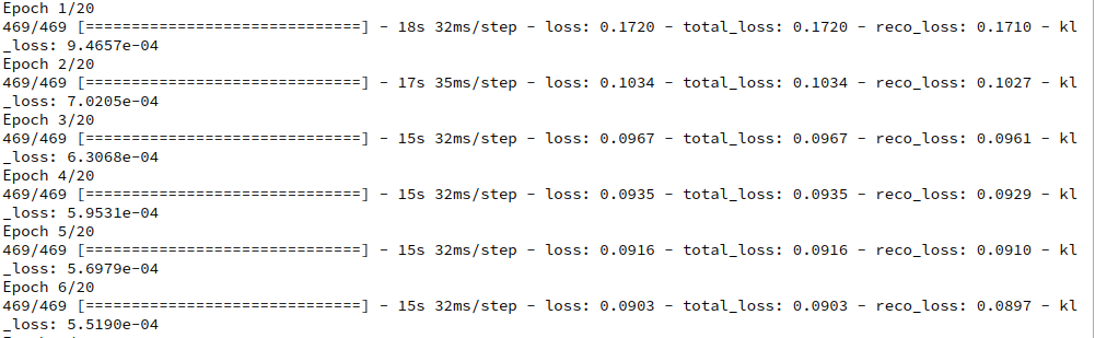
Note that I have changed the BATCH_SIZE to 256 this time; the performance got a bit better then on my old Nvidia 960 GTX:

Epoch 3/37
235/235 [==============================] - 10s 44ms/step - loss: 0.1135 - bce: 0.1091 - kl: 0.0044
Epoch 4/37
235/235 [==============================] - 10s 44ms/step - loss: 0.1114 - bce: 0.1070 - kl: 0.0044
Epoch 5/37
235/235 [==============================] - 10s 44ms/step - loss: 0.1098 - bce: 0.1055 - kl: 0.0044
Epoch 6/37
235/235 [==============================] - 10s 43ms/step - loss: 0.1085 - bce: 0.1041 - kl: 0.0044

This is comparable to data we got for our previous solution approaches. But see an additional section on performance below.

Some results

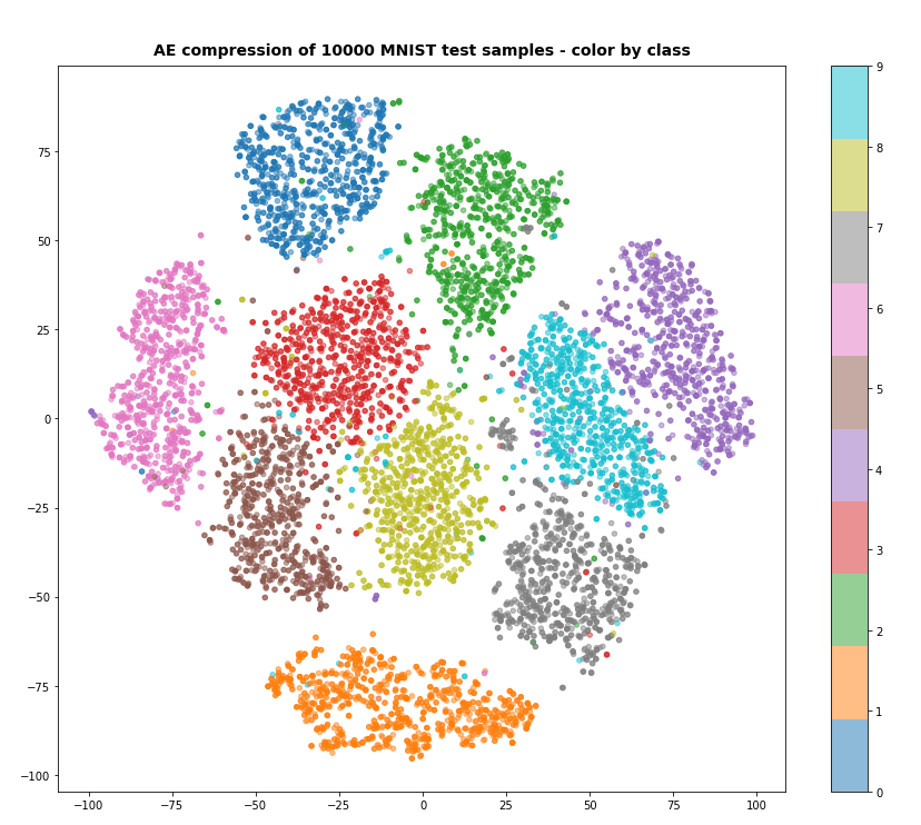
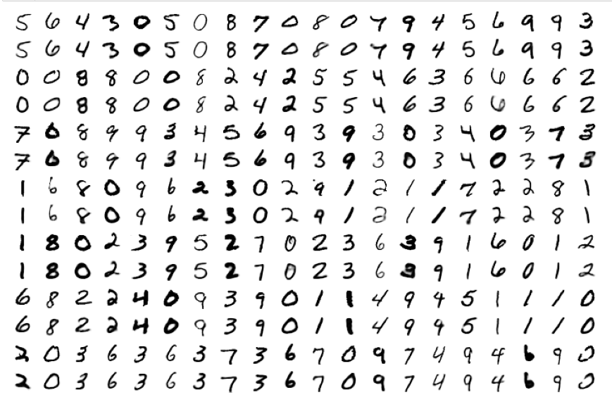
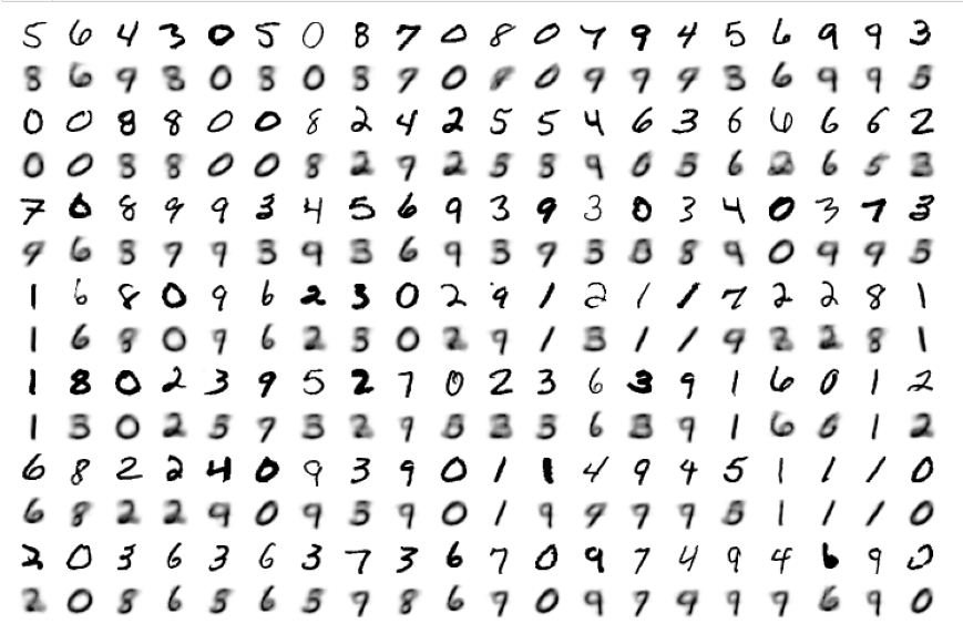
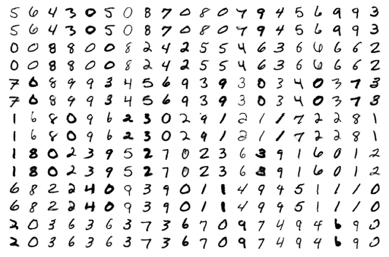
As in the last posts I show some results for the MNIST data without many comments. The first plot proves the reconstruction abilities of the VAE for a dimension z-dim=12 of the latent space.

MNIST with z-dim=12 and fact=6.5e-4

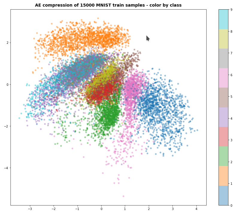
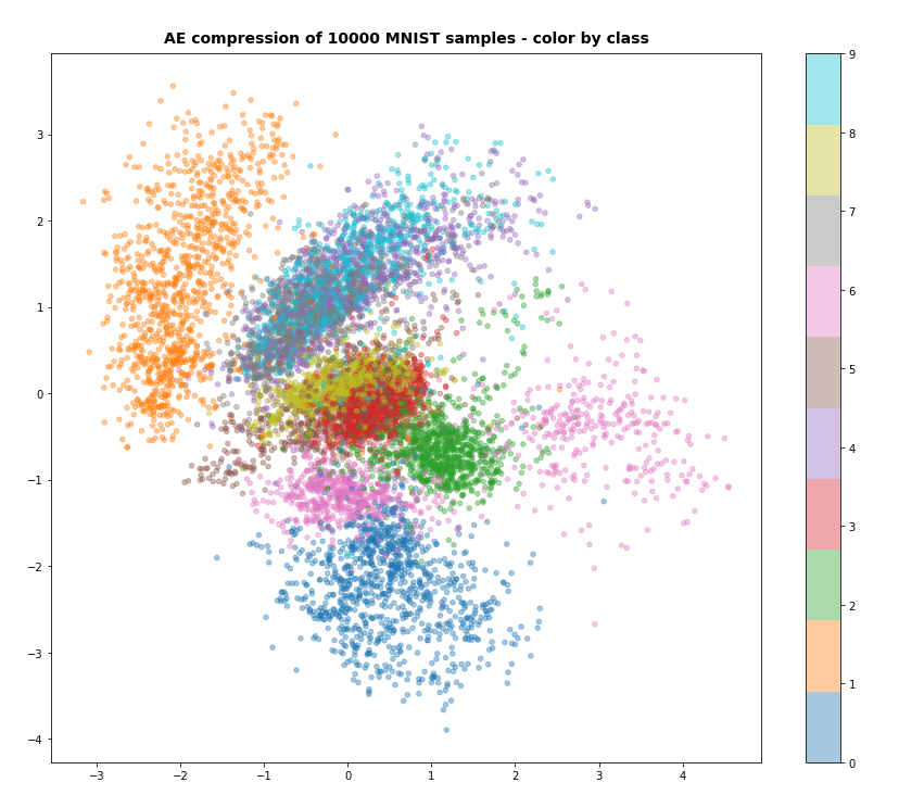
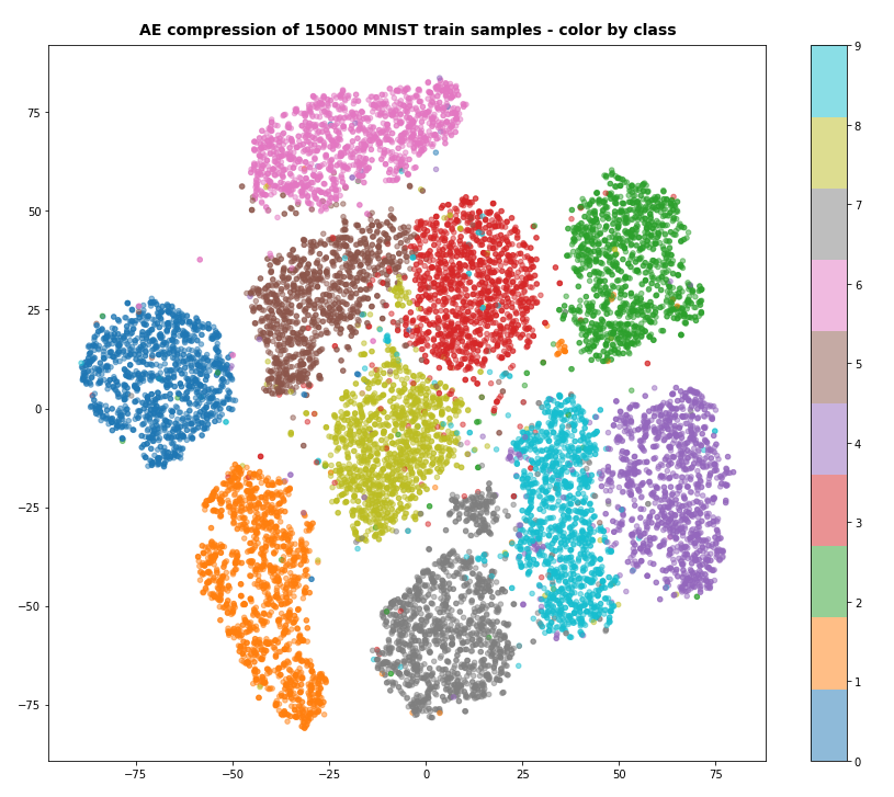
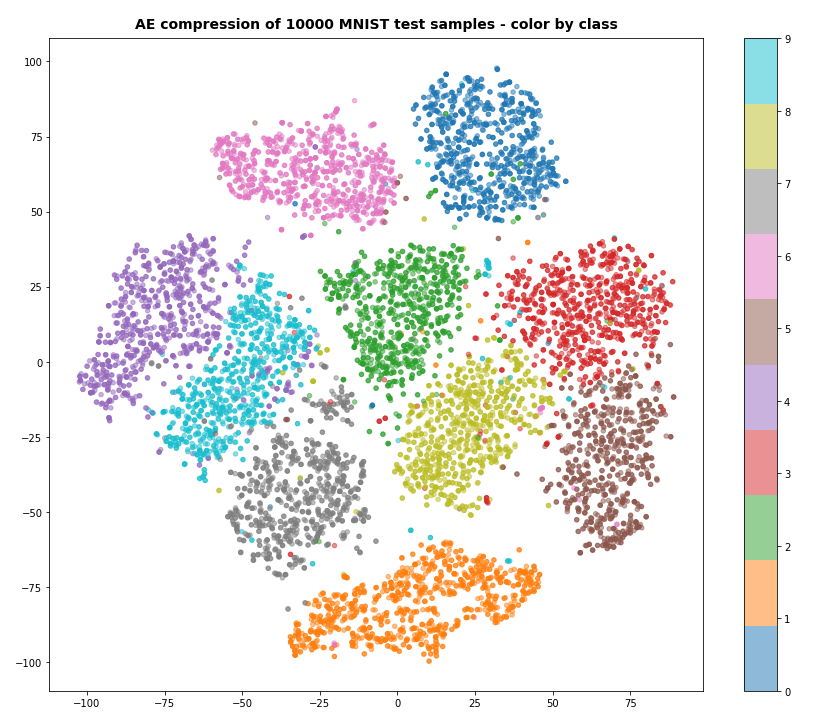
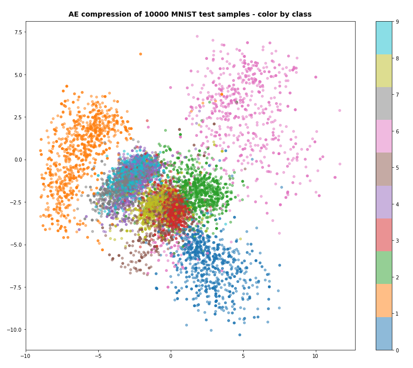
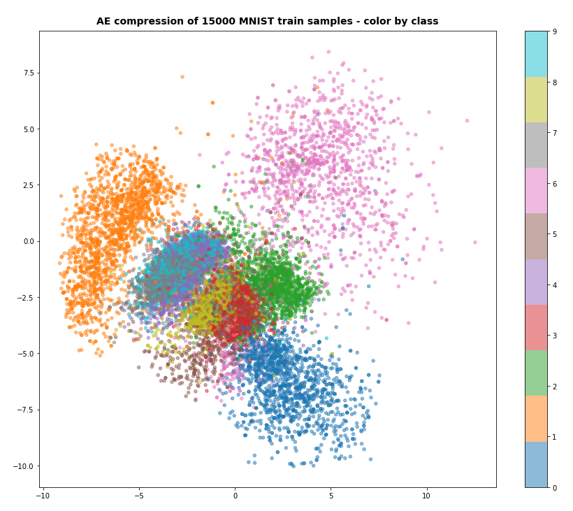
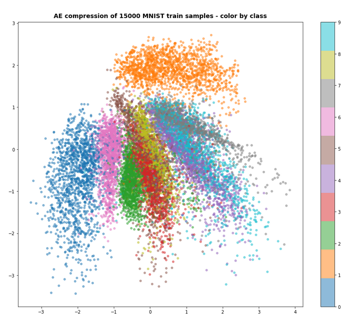
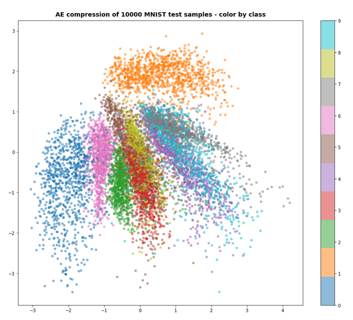
For z_dim=2 we get a reasonable data point distribution in the latent space due to the KL loss, but the reconstruction ability suffers, of course:

MNIST with z-dim=2 and fact=6.5e-4 – train data distribution in the z-space

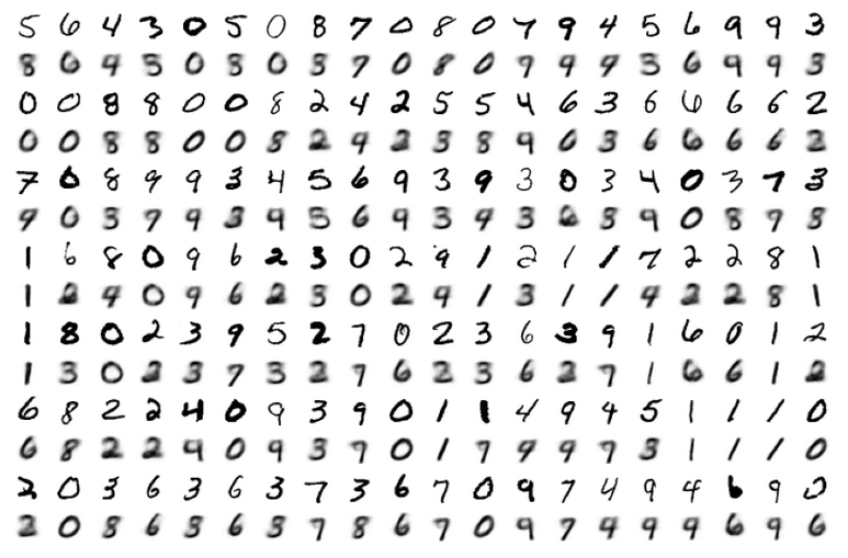
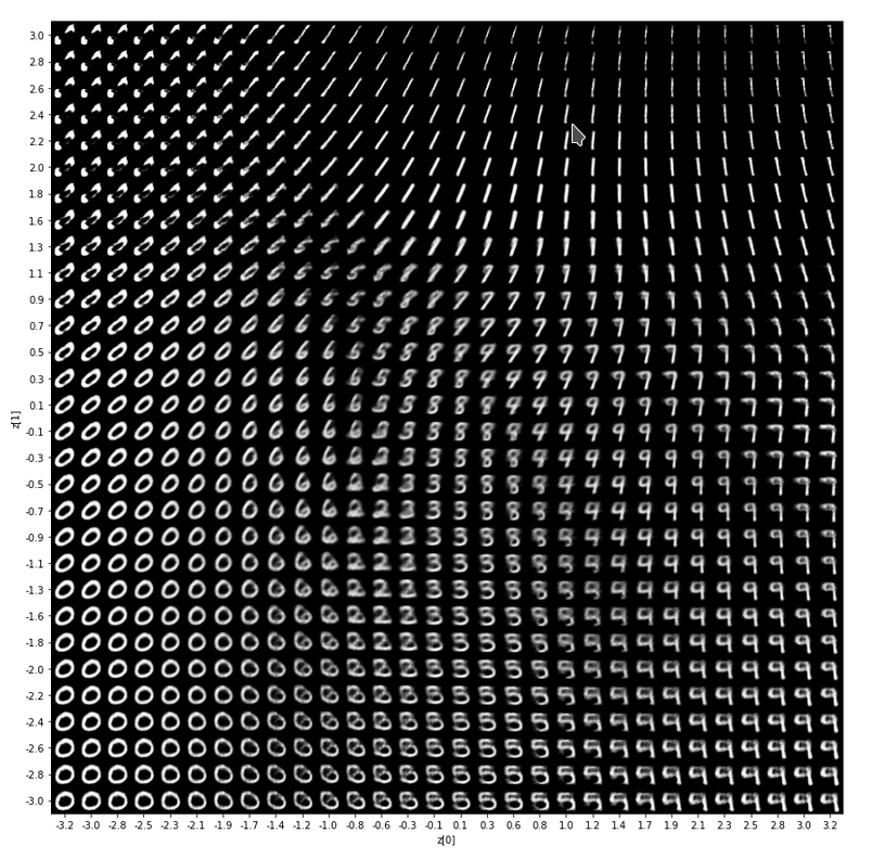
For a dimension of z_dim=2 of the latent space and MNIST data we get the following reconstruction chart for data points in a region around the latent space’s origin


A strange performance problem when no class is used

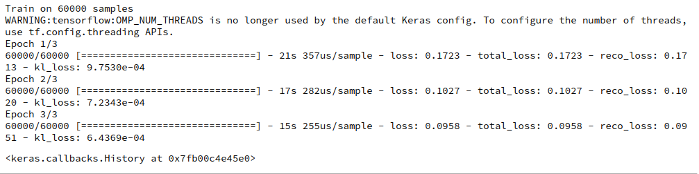
I also tested a version of the approach with model.add_loss() without encapsulating everything in a class. But with the same definition of the Encoder, the Decoder, the model, etc. But all variables as e.g. mu, log_var were directly kept as data of and in the Jupyter notebook. Then a call

n_epochs      = 3
batch_size    = 128
initial_epoch = 0
vae.fit( x_train[0:60000], 
         x_train[0:60000],   # entscheidend ! 
         batch_size=batch_size,
         shuffle=True, 
         epochs = n_epochs, 
         initial_epoch = initial_epoch 
       )

reduced the performance by a factor of 1.5. I have experimented quite a while. But I have no clue at the moment why this happens and how the effect can be avoided. I assume some strange data handling or data transfer between the Jupyter notebook and the graphics card. I can provide details if some developer is interested.

But as one should encapsulate functionality in classes anyway I have not put efforts in a detail analysis.

Conclusion

In this article we have studied an approach to handle the Kullback-Leibler loss via the model.add_loss() functionality of Keras. We supplemented our growing class for a VAE with respective methods. All in all the approach is almost more convenient as the solution based on a special layer and layer.add_loss(); see post V.

However, there seems to exist some strange performance problem when you avoid a reasonable encapsulation in a class and do the modell setup directly in Jupyter cells and for Jupyter variables.

In the next post
Variational Autoencoder with Tensorflow – VIII – TF 2 GradientTape(), KL loss and metrics
I shall have a look at the solution approach recommended by F. Chollet.

Links

We must provide tensors explicitly to model.add_loss()
https://towardsdatascience.com/shared-models-and-custom-losses-in-tensorflow-2-keras-6776ecb3b3a9

 
Ceterum censeo: The worst fascist, war criminal and killer living today, who must be isolated, be denazified and imprisoned, is the Putler. Long live a free and democratic Ukraine!
 

Variational Autoencoder with Tensorflow – V – a customized Encoder layer for the KL loss

I continue with my series on the treatment of the KL loss of Variational Autoencoders in a Keras / TF2.8 environment:

Variational Autoencoder with Tensorflow – I – some basics
Variational Autoencoder with Tensorflow – II – an Autoencoder with binary-crossentropy loss
Variational Autoencoder with Tensorflow – III – problems with the KL loss and eager execution
Variational Autoencoder with Tensorflow – IV – simple rules to avoid problems with eager execution

In the last post it became clear that it might be a good idea to delegate the KL loss calculation to a specific layer within the Encoder model. In this post I discuss the code for such a solution. I am going to encapsulate the construction of a suitable Keras model for the VAE in a class. The class will in further posts be supplemented by more methods for different approaches compatible with TF2.x and eager execution.

The code’s structure has been influenced by the work or books of several people which I want to name explicitly: D. Foster, F. Chollet and Louis Tiao. See the references in the last section of this post.

For the data sets I later want to work with both the Encoder and the Decoder parts of the VAE shall be based upon “convolutional networks” [CNNs] and respective Keras layers. Based on a suggestions of D. Foster and F. Chollet I use a classes interface to provide the parameters of all invoked Conv2D and Conv2DTranspose layers. But in contrast to D. Foster I also indicate how to include different activation functions (e.g. SeLU). In general I also will use the Keras functional API to define and add layers to the VAE model.

Imports to make Keras model and layer classes work

Below I discuss step by step parts of the code I put into a Python module to be used later in Jupyter notebooks. First we need to import some Python modules; note that you may have to add further statements which import personal modules from paths at your local machine:

import sys
import numpy as np
import os

import tensorflow as tf
from tensorflow.keras.layers import Layer, Input, Conv2D, Flatten, Dense, Conv2DTranspose, Reshape, Lambda, \
                                    Activation, BatchNormalization, ReLU, LeakyReLU, ELU, Dropout, AlphaDropout
from tensorflow.keras.models import Model
# to be consistent with my standard loading of the Keras backend in Jupyter notebooks:  
from tensorflow.keras import backend as B      
from tensorflow.keras.optimizers import Adam

A class for a special Encoder layer

Following the ideas discussed in my last post I now add a class which later allows for the setup of a special customized Keras layer in the Encoder model. This layer will calculate the KL loss for us. To be able to do so, the implementation interface “call()” receives a variable “inputs” which contains references to the mu and var_log layers of the Encoder (see the two last posts in this series).

class My_KL_Layer(Layer):
    '''
    @note: Returns the input layers ! Required to allow for z-point calculation
           in a final Lambda layer of the Encoder model    
    '''
    # Standard initialization of layers 
    def __init__(self, *args, **kwargs):
        self.is_placeholder = True
        super(My_KL_Layer, self).__init__(*args, **kwargs)

    # The implementation interface of the Layer
    def call(self, inputs, fact = 4.5e-4):
        mu      = inputs[0]
        log_var = inputs[1]
        # Note: from other analysis we know that the backend applies tf.math.functions 
        # "fact" must be adjusted - for MNIST reasonable values are in the range of 0.65e-4 to 6.5e-4
        kl_mean_batch = - fact * B.mean(1 + log_var - B.square(mu) - B.exp(log_var))
        # We add the loss via the layer's add_loss() - it will be added up to other losses of the model     
        self.add_loss(kl_mean_batch, inputs=inputs)
        # We add the loss information to the metrics displayed during training 
        self.add_metric(kl_mean_batch, name='kl', aggregation='mean')
        return inputs

An important point is that a layer based on this class must return its input, namely the mu and var_log layers, for the z-point calculations in the final Encoder layer.

Note that we do not only add the loss to other losses of an eventual VAE model via the layer’s “add_loss()” method, but that we also ensure to get some information about the the size of the KL loss during training by adding the loss to the metrics.

A general class to setup a VAE build on CNNs for Encoder and Decoder

We now build a class to create the essential parts of a VAE. The class will provide the required flexibility and allow for future extensions comprising other TF2.x compatible solutions for KL loss calculations. (In this post we only use a customized layer to get the KL loss).
We start with the classes “__init__” function, which basically transfers saves parameters into class variables.

# The Main class 
# ~~~~~~~~~~~~~~
class MyVariationalAutoencoder():
    '''
    Coding suggestions of D. Foster and F. Chollet were modified and extended by RMO 
    @version: V0.1, 25.04 
    @change:  added b_build_all 
    @version: V0.2, 08.05 
    @change:  Handling of the KL-loss via functions (partially not working)  
    @version: V0.3, 29.05 
    @change:  Handling of the KL-loss function via a customized Encoder layer 
    '''
    
    def __init__(self
        , input_dim                  # the shape of the input tensors (for MNIST (28,28,1)) 
        , encoder_conv_filters       # number of maps of the different Conv2D layers   
        , encoder_conv_kernel_size   # kernel sizes of the Conv2D layers 
        , encoder_conv_strides       # strides - here also used to reduce spatial resolution avoid pooling layers 
                                     # used instead of Pooling layers 
        , decoder_conv_t_filters     # number of maps in Con2DTranspose layers 
        , decoder_conv_t_kernel_size # kernel sizes of Conv2D Transpose layers  
        , decoder_conv_t_strides     # strides for Conv2dTranspose layers - inverts spatial resolution
        , z_dim                      # A good start is 16 or 24  
        , solution_type  = 0         # Which type of solution for the KL loss calculation ?
        , act            = 0         # Which type of activation function?  
        , fact           = 0.65e-4   # Factor for the KL loss (0.5e-4 < fact < 1.e-3is reasonable)    
        , use_batch_norm = False     # Shall BatchNormalization be used after Conv2D layers? 
        , use_dropout    = False     # Shall statistical dropout layers be used for tregularization purposes ? 
        , b_build_all    = False  # Added by RMO - full Model is build in 2 steps 
        ):
        
        '''
        Input: 
        The encoder_... and decoder_.... variables are Python lists,
        whose length defines the number of Conv2D and Conv2DTranspose layers 
        
        input_dim : Shape/dimensions of the input tensor - for MNIST (28,28,1) 
        encoder_conv_filters:     List with the number of maps/filters per Conv2D layer    
        encoder_conv_kernel_size: List with the kernel sizes for the Conv-Layers   
        encoder_conv_strides:     List with the strides used for the Conv-Layers   

        act :  determines activation function to use (0: LeakyRELU, 1:RELU , 2: SELU)
               !!!! NOTE: !!!!
               If SELU is used then the weight kernel initialization and the dropout layer need to be special   
               https://github.com/christianversloot/machine-learning-articles/blob/main/using-selu-with-tensorflow-and-keras.md
               AlphaDropout instead of Dropout + LeCunNormal for kernel initializer
        z_dim : dimension of the "latent_space"
        solution_type : Type of solution for KL loss calculation (0: Customized Encoder layer, 
                                                                  1: model.add_loss()
                                                                  2: definition of training step with Gradient.Tape()
        
        use_batch_norm = False   # True : We use BatchNormalization   
        use_dropout    = False   # True : We use dropout layers (rate = 0.25, see Encoder)
        b_build_all    = False   # True : Full VAE Model is build in 1 step; 
                                   False: Encoder, Decoder, VAE are build in separate steps   
        '''
        
        self.name = 'variational_autoencoder'

        # Parameters for Layers which define the Encoder and Decoder 
        self.input_dim                  = input_dim
        self.encoder_conv_filters       = encoder_conv_filters
        self.encoder_conv_kernel_size   = encoder_conv_kernel_size
        self.encoder_conv_strides       = encoder_conv_strides
        self.decoder_conv_t_filters     = decoder_conv_t_filters
        self.decoder_conv_t_kernel_size = decoder_conv_t_kernel_size
        self.decoder_conv_t_strides     = decoder_conv_t_strides
        
        self.z_dim = z_dim

        # Check param for activation function 
        if act < 0 or act > 2: 
            print("Range error: Parameter " + str(act) + " has unknown value ")  
            sys.exit()
        else:
            self.act = act 
        
        # Factor to scale the KL loss relative to the Binary Cross Entropy loss 
        self.fact = fact 
        
        # Check param for solution approach  
        if solution_type < 0 or solution_type > 2: 
            print("Range error: Parameter " + str(solution_type) + " has unknown value ")  
            sys.exit()
        else:
            self.solution_type = solution_type 

        self.use_batch_norm = use_batch_norm
        self.use_dropout    = use_dropout

        # Preparation of some variables to be filled later 
        self._encoder_input  = None  # receives the Keras object for the Input Layer of the Encoder 
        self._encoder_output = None  # receives the Keras object for the Output Layer of the Encoder 
        self.shape_before_flattening = None # info of the Encoder => is used by Decoder 
        self._decoder_input  = None  # receives the Keras object for the Input Layer of the Decoder
        self._decoder_output = None  # receives the Keras object for the Output Layer of the Decoder

        # Layers / tensors for KL loss 
        self.mu      = None # receives special Dense Layer's tensor for KL-loss 
        self.log_var = None # receives special Dense Layer's tensor for KL-loss 

        # Parameters for SELU - just in case we may need to use it somewhere 
        # https://keras.io/api/layers/activations/ see selu
        self.selu_scale = 1.05070098
        self.selu_alpha = 1.67326324

        # The number of Conv2D and Conv2DTranspose layers for the Encoder / Decoder 
        self.n_layers_encoder = len(encoder_conv_filters)
        self.n_layers_decoder = len(decoder_conv_t_filters)

        self.num_epoch = 0 # Intialization of the number of epochs 

        # A matrix for the values of the losses 
        self.std_loss  = tf.TensorArray(tf.float32, size=0, dynamic_size=True, clear_after_read=False)

        # We only build the whole AE-model if requested
        self.b_build_all = b_build_all
        if b_build_all:
            self._build_all()

Note that for the present post we (can) only use “solution_type = 0” !

A method to build the Encoder

The class shall provide a method to build the Encoder. For our present purposes including a customized layer based on the class “My_KL_Layer”. This layer just returns its input – namely the layers “mu” and “var_log” for the variational calculation of z-points, but it also calculates the KL loss which is added to other model losses.

    # Method to build the Encoder
    # ~~~~~~~~~~~~~~~~~~~~~~~~~~~ 
    def _build_enc(self, solution_type = 0, fact=-1.0):
        '''
        Encoder 
        @summary: Method to build the Encoder part of the AE 
                  This will be a CNN defined by the parameters to __init__   
         
        @note:    For self.solution = 0, we add an extra layer to calculate the KL loss 
        @note:    The last layer uses a sigmoid activation to create the output 
                  This may not be compatible with some scalers applied to the input data (images)    
        '''       

        # Check whether "fact" for the KL loss shall be overwritten
        if fact < 0:
            fact = self.fact  
        
        # Preparation: We later need a function to calculate the z-points in the latent space 
        # this function will be used by an eventual Lambda layer of the Encoder 
        def z_point_sampling(args):
            '''
            A point in the latent space is calculated statistically 
            around an optimized mu for each sample 
            '''
            mu, log_var = args # Note: These are 1D tensors !
            epsilon = B.random_normal(shape=B.shape(mu), mean=0., stddev=1.)
            return mu + B.exp(log_var / 2) * epsilon

        
        # Input "layer"
        self._encoder_input = Input(shape=self.input_dim, name='encoder_input')

        # Initialization of a running variable x for individual layers 
        x = self._encoder_input

        # Build the CNN-part with Conv2D layers 
        # Note that stride>=2 reduces spatial resolution without the help of pooling layers 
        for i in range(self.n_layers_encoder):
            conv_layer = Conv2D(
                filters = self.encoder_conv_filters[i]
                , kernel_size = self.encoder_conv_kernel_size[i]
                , strides = self.encoder_conv_strides[i]
                , padding = 'same'  # Important ! Controls the shape of the layer tensors.    
                , name = 'encoder_conv_' + str(i)
                )
            x = conv_layer(x)
            
            # The "normalization" should be done ahead of the "activation" 
            if self.use_batch_norm:
                x = BatchNormalization()(x)

            # Selection of activation function (out of 3)      
            if self.act == 0:
                x = LeakyReLU()(x)
            elif self.act == 1:
                x = ReLU()(x)
            elif self.act == 2: 
                # RMO: Just use the Activation layer to use SELU with predefined (!) parameters 
                x = Activation('selu')(x) 

            # Fulfill some SELU requirements 
            if self.use_dropout:
                if self.act == 2: 
                    x = AlphaDropout(rate = 0.25)(x)
                else:
                    x = Dropout(rate = 0.25)(x)

        # Last multi-dim tensor shape - is later needed by the decoder 
        self._shape_before_flattening = B.int_shape(x)[1:]

        # Flattened layer before calculating VAE-output (z-points) via 2 special layers 
        x = Flatten()(x)
        
        # "Variational" part - create 2 Dense layers for a statistical distribution of z-points  
        self.mu      = Dense(self.z_dim, name='mu')(x)
        self.log_var = Dense(self.z_dim, name='log_var')(x)

        if solution_type == 0: 
            # Customized layer for the calculation of the KL loss based on mu, var_log data
            # We use a customized layer accoding to a class definition  
            self.mu, self.log_var = My_KL_Layer()([self.mu, self.log_var], fact=fact)
 
        # Layer to provide a z_point in the Latent Space for each sample of the batch 
        self._encoder_output = Lambda(z_point_sampling, name='encoder_output')([self.mu, self.log_var])

        # The Encoder Model 
        self.encoder = Model(self._encoder_input, self._encoder_output)

A method to build the Decoder

The following function should be self-evident; it reverses the Encoder’s operations and uses z-points of the latent space as input.

    # Method to build the Decoder
    # ~~~~~~~~~~~~~~~~~~~~~~~~~~~ 
    def _build_dec(self):
        '''
        Decoder 
        @summary: Method to build the Decoder part of the AE 
                  Normally this will be a reverse CNN defined by the parameters to __init__   
        '''       

        # Input layer - aligned to the shape of the output layer 
        self._decoder_input = Input(shape=(self.z_dim,), name='decoder_input')

        # Here we use the tensor shape info from the Encoder          
        x = Dense(np.prod(self._shape_before_flattening))(self._decoder_input)
        x = Reshape(self._shape_before_flattening)(x)

        # The inverse CNN
        for i in range(self.n_layers_decoder):
            conv_t_layer = Conv2DTranspose(
                filters = self.decoder_conv_t_filters[i]
                , kernel_size = self.decoder_conv_t_kernel_size[i]
                , strides = self.decoder_conv_t_strides[i]
                , padding = 'same' # Important ! Controls the shape of tensors during reconstruction
                                   # we want an image with the same resolution as the original input 
                , name = 'decoder_conv_t_' + str(i)
                )
            x = conv_t_layer(x)

            # Normalization and Activation 
            if i < self.n_layers_decoder - 1:
                # Also in the decoder: normalization before activation  
                if self.use_batch_norm:
                    x = BatchNormalization()(x)
                
                # Choice of activation function
                if self.act == 0:
                    x = LeakyReLU()(x)
                elif self.act == 1:
                    x = ReLU()(x)
                elif self.act == 2: 
                    #x = self.selu_scale * ELU(alpha=self.selu_alpha)(x)
                    x = Activation('selu')(x)
                
                # Adaptions to SELU requirements 
                if self.use_dropout:
                    if self.act == 2: 
                        x = AlphaDropout(rate = 0.25)(x)
                    else:
                        x = Dropout(rate = 0.25)(x)
                
            # Last layer => Sigmoid output 
            # => This requires scaled input => Division of pixel values by 255
            else:
                x = Activation('sigmoid')(x)

        # Output tensor => a scaled image 
        self._decoder_output = x

        # The Decoder model 
        self.decoder = Model(self._decoder_input, self._decoder_output)

Note that we do not include any loss calculations in the Decoder model. The main loss – namely according to the “binary cross entropy” will later be added to the “fit()” method of the full Keras based VAE model.

The full VAE model

We have already created two Keras models for the Encoder and Decoder. We now combine them to the full VAE model and save this model in a variable of the object derived from our class.

    # Function to build the full AE
    # ~~~~~~~~~~~~~~~~~~~~~~~~~~~~~
    def _build_VAE(self):     
        model_input  = self._encoder_input
        model_output = self.decoder(self._encoder_output)
        self.model = Model(model_input, model_output, name="vae")

    # Function to build full AE in one step if requested
    # ~~~~~~~~~~~~~~~~~~~~~~~~~~~~~~~~~~~~~~~~~~~~~~~~~~
    def _build_all(self):
        self._build_enc()
        self._build_dec()
        self._build_VAE()

Compilation

For our present solution with the customized layer for the KL loss we now provide a matching “compile()” function:

    # Function to compile VA-model with a KL-layer in the Encoder 
    # ~~~~~~~~~~~~~~~~~~~~~~~~~~~~~~~~~~~~~~~~~~~~~~~~~~~~~~~~~
    def compile_for_KL_Layer(self, learning_rate):
        if self.solution_type != 0: 
            print("The compile_L() function is only compatible with solution_type = 0")
            sys.exit()
        self.learning_rate = learning_rate
        # Optimizer 
        optimizer = Adam(learning_rate=learning_rate)
        self.model.compile(optimizer=optimizer, loss="binary_crossentropy",
                           metrics=[tf.keras.metrics.BinaryCrossentropy(name='bce')])

This is the place where we include the main contribution to the loss – namely by a “binary cross-entropy” calculation with respect to the differences between the original input tensor top our model and its output tensor. We had to use the function BinaryCrossentropy(name=’bce’) to be able to give the respective output during training a short name. All in all we expect an output during training comprising:

  • the total loss
  • the contribution from the binary_crossentropy
  • the KL contribution

A method for training

We are almost finished. We just need a matching method for starting the training via calling the “fit()“-function of our Keras based VAE model:

    def train_model_with_KL_Layer(self, x_train, batch_size, epochs, initial_epoch = 0):
        self.model.fit(     
            x_train
            , x_train
            , batch_size = batch_size
            , shuffle = True
            , epochs = epochs
            , initial_epoch = initial_epoch
        )

Note that we called the same “x_train” batch of samples twice: The standard “y” output “labels” actually are the input samples (which is, of course, the core characteristic of AEs). We shuffle data during training.

Why use a special function of the class at all and not directly call fit() from Jupyter notebook cells?
Well, at this point we could include multiple other things as custom callbacks (e.g. for special output or model saving) and a scheduler. See e.g. the code of D. Foster at his Github site for variants. For the sake of briefness I skip these techniques in my post.

Jupyter cells to use our class

Let us see how we can use our carefully crafted class with a Jupyter notebook. As I personally gather Python modules (via Eclipse PyDev) in some special folders, I first have to add a path:

Cell 1:

import sys
# !!! ADAPT to YOUR needs !!!!! 
sys.path.append("/projects/GIT/ml_4/")
print(sys.path)

Of course, you must adapt this path to your personal situation.

The next cell contains module imports
Cell 2

import numpy as np
import time 
import os
import sklearn # could be used for scalers
import matplotlib as mpl
from matplotlib import pyplot as plt
from matplotlib.colors import ListedColormap
import matplotlib.patches as mpat 

# tensorflow and keras 
import tensorflow as tf
from tensorflow import keras as K
from tensorflow.python.keras import backend as B 
from tensorflow.keras import models
from tensorflow.keras import layers
from tensorflow.keras import regularizers
from tensorflow.keras import optimizers
from tensorflow.keras import metrics
from tensorflow.keras.datasets import mnist
from tensorflow.keras.optimizers import schedules
from tensorflow.keras.utils import to_categorical
from tensorflow.python.client import device_lib
from tensorflow.keras.datasets import mnist

# My VAE-class 
from my_AE_code.models.My_VAE import MyVariationalAutoencoder

I then suppress some warnings regarding my Nvidia card and list the available Cuda devices.

Cell 3


# Suppress some TF2 warnings on negative NUMA node number
# see https://www.programmerall.com/article/89182120793/
os.environ['TF_CPP_MIN_LOG_LEVEL'] = '3'  # or any {'0', '1', '2'}
tf.config.experimental.list_physical_devices()

We then control resource usage:
Cell 4

# Restrict to GPU and activate jit to accelerate 
# IMPORTANT NOTE: To change any of the following values you MUT restart the notebook kernel ! 
b_tf_CPU_only      = False   # we want to work on a GPU  
tf_limit_CPU_cores = 4 
tf_limit_GPU_RAM   = 2048

if b_tf_CPU_only: 
    tf.config.set_visible_devices([], 'GPU')   # No GPU, only CPU 
    # Restrict number of CPU cores
    tf.config.threading.set_intra_op_parallelism_threads(tf_limit_CPU_cores)
    tf.config.threading.set_inter_op_parallelism_threads(tf_limit_CPU_cores)
else: 
    gpus = tf.config.experimental.list_physical_devices('GPU')
    tf.config.experimental.set_virtual_device_configuration(gpus[0], 
    [tf.config.experimental.VirtualDeviceConfiguration(memory_limit = tf_limit_GPU_RAM)])

# JiT optimizer 
tf.config.optimizer.set_jit(True)

Let us load MNIST for test purposes:
Cell 5

def load_mnist():
    (x_train, y_train), (x_test, y_test) = mnist.load_data()

    x_train = x_train.astype('float32') / 255.
    x_train = x_train.reshape(x_train.shape + (1,))
    x_test = x_test.astype('float32') / 255.
    x_test = x_test.reshape(x_test.shape + (1,))

    return (x_train, y_train), (x_test, y_test)

(x_train, y_train), (x_test, y_test) = load_mnist()

Provide the VAE setup variables to our class:
Cell 6

z_dim = 2
vae = MyVariationalAutoencoder(
    input_dim = (28,28,1)
    , encoder_conv_filters = [32,64,128]
    , encoder_conv_kernel_size = [3,3,3]
    , encoder_conv_strides = [1,2,2]
    , decoder_conv_t_filters = [64,32,1]
    , decoder_conv_t_kernel_size = [3,3,3]
    , decoder_conv_t_strides = [2,2,1]
    , z_dim = z_dim
    , act   = 0
    , fact  = 5.e-4
)

Set up the Encoder:
Cell 7

# overwrite the KL fact from the class 
fact = 2.e-4 
vae._build_enc(fact=fact)
vae.encoder.summary()

Build the Decoder:
Cell 8

vae._build_dec()
vae.decoder.summary()

Build the VAE model:
Cell 9

vae._build_VAE()
vae.model.summary()

Compile
Cell 10

LEARNING_RATE = 0.0005
vae.compile_for_KL_Layer(LEARNING_RATE)

Train / fit the model to the training data
Cell 11

BATCH_SIZE = 128
EPOCHS = 6     # for real runs ca. 40 
INITIAL_EPOCH = 0
vae.train_model_with_KL_Layer(     
    x_train[0:60000]
    , batch_size = BATCH_SIZE
    , epochs = EPOCHS
    , initial_epoch = INITIAL_EPOCH
)

For the given parameters I got the following output on my old GTX960

Epoch 1/6
469/469 [==============================] - 12s 24ms/step - loss: 0.2613 - bce: 0.2589 - kl: 0.0024
Epoch 2/6
469/469 [==============================] - 12s 25ms/step - loss: 0.2174 - bce: 0.2159 - kl: 0.0015
Epoch 3/6
469/469 [==============================] - 11s 23ms/step - loss: 0.2100 - bce: 0.2085 - kl: 0.0015
Epoch 4/6
469/469 [==============================] - 11s 23ms/step - loss: 0.2057 - bce: 0.2042 - kl: 0.0015
Epoch 5/6
469/469 [==============================] - 11s 23ms/step - loss: 0.2034 - bce: 0.2019 - kl: 0.0015
Epoch 6/6
469/469 [==============================] - 11s 23ms/step - loss: 0.2019 - bce: 0.2004 - kl: 0.0015

So 11 secs for an epoch of 60,000 samples with batch-size = 128 is a reference point. Note that this is obviously faster than what we got for the solution discussed in the last post.

Just to give you an impression of other results:
For z_dim = 2, fact = 2.e-4 and 60 epochs I got something like the following data point distribution in the latent space:

I shall discuss more results – also for other test data sets – in future posts in this blog.

Conclusion

In this post we have build a class to set up a VAE based on an Encoder and a Decoder model with Conv2D and Conv2dTranspose layers. We delegated the calculation of the KL loss to a customized layer of the Encoder, whilst the main loss contribution was defined in form of a binary-crossentropy evaluation with the help of the fit()-function of the VAE model. All loss contributions were displayed as “metrics” elements during training. The presented solution is fully compatible with Tensorflow 2.8 and eager execution. It is in my opinion also elegant and very Keras oriented as all important operations are encapsulated in a continuous sequence of layers. We also found this to be a relatively fast solution.

In the next post of this series
Variational Autoencoder with Tensorflow – VI – KL loss via tensor transfer and multiple output
we are going to use our class to adapt an older suggestion of D.Foster to the requirements of TF2.8.

References

F. Chollet, Deep Learning mit Python und Keras, 2018, 1-te dt. Auflage, mitp Verlags GmbH & Co.KG, Frechen

D. Foster, “Generatives Deep Learning”, 2020, 1-te dt. Auflage, dpunkt Verlag, Heidelberg in Kooperation mit Media Inc.O’Reilly, ISBN 978-3-960009-128-8. See Kap. 3 and the VAE code published at
https://github.com/davidADSP/GDL_code/

Louis Tiao, “Implementing Variational Autoencoders in Keras: Beyond the Quickstart Tutorial”, 2017, http://louistiao.me/posts/implementing-variational-autoencoders-in-keras-beyond-the-quickstart-tutorial/

Recommendation: The article of L. Tiao is not only interesting regarding Keras modularity. I like it very much also for his mathematical depth. I highly recommend his article as a source of inspiration, especially with respect to alternative divergences. Please, also follow Tiao’s list of well selected literature references.

And before I forget it:
Ceterum censeo: The worst living fascist and war criminal today, who must be isolated, denazified and imprisoned, is the Putler.

Variational Autoencoder with Tensorflow – IV – simple rules to avoid problems with eager execution

In the last posts of this series

Variational Autoencoder with Tensorflow – I – some basics
Variational Autoencoder with Tensorflow – II – an Autoencoder with binary-crossentropy loss
Variational Autoencoder with Tensorflow – III – problems with the KL loss and eager execution

we have seen that it is a bit more difficult to set up a Variational Autoencoder [VAE] with Keras and Tensorflow 2.8 than a pure Autoencoder [AE]. One of the reasons is that we need to include extra layers for a statistical variation of z-points around mean values “mu” with a variance “var” for each sample. In addition a special loss – the Kullback Leibler loss – must be taken into account besides a binary-crossentropy loss to optimize the “mu” and “log_var” values in parallel to a good reconstruction ability of the Decoder.

In the last post we also saw that a too conservative handling of the Kullback-Leibler divergence may lead to problems with the “eager execution mode” of present Tensorflow 2 versions.

In this post I shall first show you how to remedy the specific problem presented in the last post. Sometimes solutions are easy to achieve … :-). But we should also understand the reason for the problem. Some basic considerations will help. Afterward we have a brief look at the performance. At last, we summarize our experiences in some simple rules.

Eager execution instead of a graph

The next statements are according to my present understanding:
When we designed layered structures of ANNs and related operations with TF 1.x and Keras, Tensorflow built a graph as an intermediate product. The graph contained all mathematical operations in a symbolic way – including the calculation of partial derivatives and gradients. The analysis of the graph by TF afterward lead to a defined sequence of real numerical operations. It is clear that the full knowledge of the graph offers the chance for an optimization of the intended operations, e.g. for ANN-training and error back propagation based on gradient components (=partial derivatives with respect to trainable variables of an ANN, mostly weights). Potential disadvantages of graphs are: Their analysis takes time and it has to be completed before any numerical operations can be started in the background. This in turn means that we cannot test code directly within a sequence of Python statements.

In an eager execution environments planned operations instead are evaluated immediately as the related tensors occur and in case of neural networks as their relation to (weight) variables of interest are properly defined. This includes the calculation of partial derivatives (see my post on error backward calculation for MLPs) with respect to these weights. A requirement is that the operations (= mathematical functions) on specific tensors (represented by matrices) must be well defined. Such operations can be defined by a TF2 math operations directly applied to user defined tensors in a Python statement. But they can also be encapsulated in user or Keras defined functions and combined in complicated ways – provided that it is clear how the chain rule must be applied. As the relation between the trainable variables of neighboring Keras layers in a neural network is well defined also the gradient contributions of two neighbor layers to any loss function is properly defined – and can be calculated already during the forward pass through a neural network. At least in principle we can get resulting tensor values directly or asap during forward propagation wherever possible.

As there are no graphs in eager execution, automatic differentiation based on a graph analysis is not possible without some help. Something has to track operations and functions applied to tensors and record resulting gradient components (i.e. partial derivative values) during a forward pass through a complicated network such that the derivatives can be used during error back-propagation. The tool for this is Gradient.Tape().

A general interface to TF 2.0 like Keras has to incorporate and use Gradient.Tape() internally. While trainable variables like those of a Keras layer can automatically be watched by Gradient.Tape(), specific user defined operations have to be explicitly registered with Gradient.Tape() if you cannot use some Keras model or Keras layer options. However, when you use Keras to define your models gradient related calculations are done directly already during the forward pass through a network. Whilst moving forward through a defined network’s layers gradient contributions (partial derivatives) are evaluated obeying the chain rule across variables of previous layers, of course. The resulting gradient contributions can later be used and properly combined for error backward calculation.

A remedy to the problem with the failed approach for the KL loss

Just as a reminder: In the last post I introduced a special layer to take care of the KL loss according to a recipe of F. Chollet in his book on Deep Learning of 2017 (see the precise reference at the end of my last post):

Customized Keras layer class:

class CustVariationalLayer (Layer):
    
    def vae_loss(self, x_inp_img, z_reco_img):
        # The references to the layers are resolved outside the function 
        x = B.flatten(x_inp_img)   # B: tensorflow.keras.backend
        z = B.flatten(z_reco_img)
        
        # reconstruction loss per sample 
        # Note: that this is averaged over all features (e.g.. 784 for MNIST) 
        reco_loss = tf.keras.metrics.binary_crossentropy(x, z)
        
        # KL loss per sample - we reduce it by a factor of 1.e-3 
        # to make it comparable to the reco_loss  
        kln_loss  = -0.5e-4 * B.mean(1 + log_var - B.square(mu) - B.exp(log_var), axis=1) 
        # mean per batch (axis = 0 is automatically assumed) 
        return B.mean(reco_loss + kln_loss), B.mean(reco_loss), B.mean(kln_loss) 
           
    def call(self, inputs):
        inp_img = inputs[0]
        out_img = inputs[1]
        total_loss, reco_loss, kln_loss = self.vae_loss(inp_img, out_img)
        # We add the loss from the layer 
        self.add_loss(total_loss, inputs=inputs)
        self.add_metric(total_loss, name='total_loss', aggregation='mean')
        self.add_metric(reco_loss, name='reco_loss', aggregation='mean')
        self.add_metric(kln_loss, name='kl_loss', aggregation='mean')
        
        return out_img  # not really used in this approach  

This layer was added on top of the sequence of Encoder and Decoder: Encoder => Decoder => KL_layer.

enc_output = encoder(encoder_input)
decoder_output = decoder(enc_output)
KL_layer = CustomVariationalLayer()([mu, log_var, encoder_input, decoder_output])
vae = Model(encoder_input, KL_layer, name="vae")

This lead to an error.

Making it work …

Can we remedy the approach above by some simple means? Yes, we can. I first list the solution’s code, then discuss it:

# SOLUTION I: Custom Layer for total and KL loss 
# ~~~~~~~~~~~~~~~~~~~~~~~~~~~~~~~~~~~~~~~~~~~~~~~
class CustomVariationalLayer (Layer):
    def vae_loss(self, mu, log_var, inp_img, out_img):
        bce = tf.keras.losses.BinaryCrossentropy()    
        reco_loss = bce(inp_img, out_img)
        kln_loss  = -0.5e-4 * B.mean(1 + log_var - B.square(mu) - B.exp(log_var), axis=1) # mean per sample 
        return B.mean(reco_loss + kln_loss), B.mean(reco_loss), B.mean(kln_loss) # means per batch 
    
    def call(self, inputs):
        mu = inputs[0]
        log_var = inputs[1]; inp_img = inputs[2]; out_img = inputs[3]
        total_loss, reco_loss, kln_loss = self.vae_loss(mu, log_var, inp_img, out_img)
        self.add_loss(total_loss, inputs=inputs)
        self.add_metric(total_loss, name='total_loss', aggregation='mean')
        self.add_metric(reco_loss, name='reco_loss', aggregation='mean')
        self.add_metric(kln_loss, name='kl_loss', aggregation='mean')
        return inputs[3]  # Not used   

What is the main difference? Answer: We explicitly provided the tensors as input variables of the function vae_loss()!
Why does it help?

Well, TF2 has to prepare and calculate partial derivatives according to the chain rule of differential calculus. What would you yourself want to know on a mathematical level? You would write down any complicated function with further internal operation as a function of well defined arguments! So: We must tell TF2.x explicitly what the variables, namely tensors, of any defined function or operation are to apply the chain rule properly – whatever we do inside the function. When we had graphs this analysis could be done during the analysis of the graph. However, with eager execution we have to know all rules for the affected tensors when they occur and are operated upon. If we operate on tensors via a function, TF2 needs the functions’s arguments to handle the function and following operations properly according to the chain rule. (The tensors themselves at a layer depend, of course, on matrix operations involving trainable parameters, namely weights with respect to a previous layer, and derivatives of activation functions). By the way: The output of the functions must be defined equally well.

In our original approach the function’s input was not defined. It obviously matters with TF2.x!

As a consequence the summary of our VAE model has become longer than in the last post:

What results do we get for z_dim = 16 and z_dim=2?

For our solution we compile and train like follows:

vae.compile(optimizer=Adam(), loss=None)
n_epochs = 40
batch_size = 128
vae.fit(x=x_train, y=None, shuffle=True, 
        epochs = n_epochs, batch_size=batch_size)

Note that we do not provide any “y” to fit against. The costs are already fully defined by our special customized layer. If we, however, had used the binary_crossentropy loss in the compile statement we would have had to provide predicted tensors; see below.

On a Nvidia 960 GTX the calculation proceeds for some epochs like:

After 40 epochs we get with t-SNE well separated clusters for the test-data:

More interesting is the result for z_dim = 2, as we expect a more confined usage of the available z-space. And indeed, if we raise the factor in front of the KL loss e.g. to 6.5e-4, we get something like

With the exception of “6”-digits the samples use the space between -4 < y < 3.5 and -3 < x < 4.5 in z-space. This area is smaller by roughly a factor of 4 (i.e. 2 in each direction) than the space used of a standard Autoencoder (see the 1st post of this series). So, the KL loss shows an effect.

Performance?

However, our new approach is not as fast as it could be. What can we do to optimize? First we can get rid of the extra function in the layer. We could work directly on the tensors in the call function. A further step would be to focus only on the KL loss. Why not let Keras organize the stuff for binary_crossentropy? But all this would not change our performance much.

The real problem in our case (suggested by the master, F. Chollet, himself in an older book) is an inefficient layer structure: We cannot deal directly with the partial derivatives where the tensors appear – namely in the Encoder. Thereby an otherwise possible sequence of linear algebra operations (matrix operations), which could be optimized for error back propagation, is interrupted in a complicated way at the special layers mu and log_var. So, it appears that a strategy which would encapsulate our KL loss calculation in a specific layer of the Encoder would boost performance. This is indeed the case. I will show the solution in my next post, but give you an idea of the performance gain, already:

Instead of 15 secs as above per epoch we are going to need only 10 to 11 secs.

What have we learned? Two rules …

I see two basic rules which I personally was not aware of before:

  • If you need to perform complex calculations based on layer related tensors to get certain loss contributions and if you want to use the result with pre-defined Keras functions as “layer.add_loss()” and “model.add_loss()” then provide the result tensors explicitly as input variables to the Keras functions. You can use separate personal functions ahead to perform the required tensor operations, but these functions must also have all layer based tensors as explicit input variables and an explicit tensor as output.
  • If possible apply your calculations within special layers closely following he layers which provide the tensors your loss contribution depends on. Best before new trainable variables are introduced. Use the special layer’s add_loss() method. Try to verify that your operations fit into a layer related sequence of matrix operations whose values are needed later for error backward propagation, but are calculated already during the forward pass.

The first rule can be symbolized by something like

# Model definition
... 
layer1 = Keras_defined_layer()   #e.g. Dense()  
...
layer2 = Keras_defined_layer()   # e.g. Activation() 
...
model = Model(....)

# cost calculation 
res_tensor_cost_contribution = complex_personal_function( layer1, layer2 )   
model.add_loss(res_tensor_cost_contribution) 

An additional rule may be:

  • Try if TF2 math tensor operations are faster than tensorflow.keras.backend operations. I do not think so, but …

Three strategies to avoid problems with TF 2.8 and VAEs

In the following posts I am going to pursue three ways to handle the KL loss:

  1. We add a layer to the Encoder and perform the required KL loss calculation there. We have to take care of a proper output of such a layer not to disrupt the combination of the Encoder with the Decoder. This is in my opinion the most elegant and also the fastest option. It also fits perfectly into the Keras philosophy of defining models via layers. And we can use the Keras compile() and fit() functions seamlessly.
  2. We calculate the loss after combining the Encoder and Decoder to a VAE-model – and add the KL loss to our VAE model via its add_loss() method. This is a possible and well defined variant as it separates the loss operations from the VAE’s layer structure. Very similar to what we did above – but probably not the fastest method for VAEs.
  3. We use Gradient.Tape() directly to define an individual training step for our Keras based VAE model. This method will prove to be a fast and very flexible method. But in a way it leaves the path of using only Keras layers to define and fit neural network models. Nevertheless: Although it requires a different view on the Keras interface to TF2.x it is certainly the future we should get used to – even if we are no Keras and TF specialists.

Conclusion

In this post we saw that some old recipes for VAE design with Keras can still be used with some minor modifications. Two rules show us different ways to make Keras based VAE-ANNs work together with TF2.8. In the next post of this series
Variational Autoencoder with Tensorflow – V – a customized Encoder layer for the KL loss
we shall build a VAE with an Encoder layer to deal with the Kullback-Leibler loss.