
In the last post of this series
Variational Autoencoder with Tensorflow – I – some basics
I have briefly discussed the basic elements of a Variational Autoencoder [VAE]. Among other things we identified an Encoder, which transforms sample data into z-points in a low dimensional “latent space”, and a Decoder which reconstructs objects in the original variable space from z-points.
In the present post I want to demonstrate that a simple Autoencoder [AE] works as expected with Tensorflow 2.8 [TF2]. In contrast to certain versions of Variational Autoencoders which we shall test in the next post. For our AE we use the “binary cross-entropy” as a suitable loss to compare reconstructed MNIST images with the original ones.
A simple AE
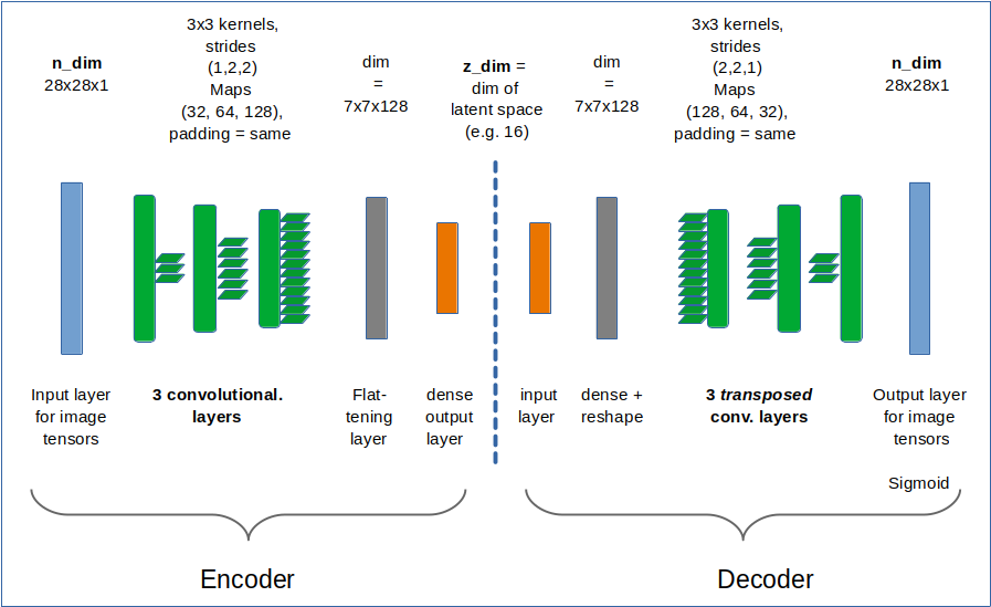
I use the functional Keras API to set up the Autoencoder. Later on we shall encapsulate everything in a class, but lets keep things simple for the time being. We design both the Encoder and the Decoder as CNNs and use properly configured Conv2D and Conv2DTranspose layers as their basic elements.
Required Imports
# tensorflow and keras
import tensorflow as tf
from tensorflow import keras as K
from tensorflow.keras import backend as B
from tensorflow.keras.models import Model
from tensorflow.keras import regularizers
from tensorflow.keras.optimizers import Adam
from tensorflow.keras import metrics
from tensorflow.keras.layers import Input, Conv2D, Flatten, Dense, Conv2DTranspose, Reshape, Lambda, \
                                    Activation, BatchNormalization, ReLU, LeakyReLU, ELU, Dropout, \
                                    AlphaDropout, Concatenate, Rescaling, ZeroPadding2D

from tensorflow.keras.utils import to_categorical
from tensorflow.keras.optimizers import schedules
z_dim and the Encoder defined with the functional API
We set the dimension of the “latent space” to z-dim = 16.
This allows for a very good reconstruction of images in the MNIST case.
z_dim = 16
encoder_input = Input(shape=(28,28,1)) # Input images pixel values are scaled by 1./255.
x = encoder_input
x = Conv2D(filters = 32, kernel_size = 3, strides = 1, padding='same')(x)
x = LeakyReLU()(x)
x = Conv2D(filters = 64, kernel_size = 3, strides = 2, padding='same')(x)
x = LeakyReLU()(x)
x = Conv2D(filters = 128, kernel_size = 3, strides = 2, padding='same')(x)
x = LeakyReLU()(x)
shape_before_flattening = B.int_shape(x)[1:]  # B: Keras backend
x = Flatten()(x)
encoder_output = Dense(self.z_dim, name='encoder_output')(x)
encoder = Model([encoder_input], [encoder_output], name="encoder")
This is almost an overkill for something as simple as MNIST data. The Decoder reverses the operations. To do so it uses Conv2DTranspose layers.
The Decoder
dec_inp_z      = Input(shape=(z_dim))
x = Dense(np.prod(shape_before_flattening))(dec_inp_z)
x = Reshape(shape_before_flattening)(x)
x = Conv2DTranspose(filters=64, kernel_size=3, strides=2, padding='same')(x)
x = LeakyReLU()(x)
x = Conv2DTranspose(filters=32, kernel_size=3, strides=2, padding='same')(x)
x = LeakyReLU()(x)
x = Conv2DTranspose(filters=1,  kernel_size=3, strides=1, padding='same')(x)
x = LeakyReLU()(x)
# Output into a region of 0 to 1 - requires a one hot encoding of classes
# and scaling of pixel values of the input samples to [0, 1]
x = Activation('sigmoid')(x)
decoder_output = x
decoder = Model([dec_inp_z], [decoder_output], name="decoder")
The full AE-model
ae_input  = encoder_input
ae_output = decoder(encoder_output)
AE = Model(ae_input, ae_output, name="AE")
That was easy! Now we compile:
AE.compile(optimizer=Adam(learning_rate = 0.0005), loss=['binary_crossentropy'])
I use the “binary_crossentropy” loss function to evaluate and punish differences between the reconstructed image and the original. Note that we need to scale pixel values of input images (as MNIST images) down to a value range between [0, 1] due to using a sigmoid activation function at the output layer of the Decoder.
Using “binary cross-entropy” leads to a better and faster convergence of the training process:
Training and results of the Autoencoder for MNIST samples
Eventually, we can train our model:
n_epochs = 40
batch_size = 128
AE.fit( x=x_train, y=x_train, shuffle=True,
         epochs = n_epochs, batch_size=batch_size)
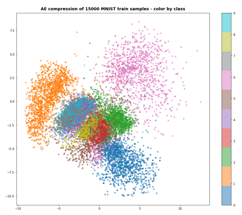
After 40 training steps we can visualize the resulting data clusters in z-space. To get a 2-dimensional plot out of 16-dimensional data requires the use of t-SNE. For 15.000 training data (out of 60.000) we get:
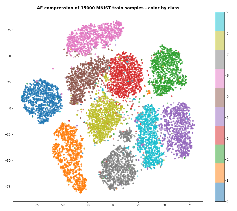
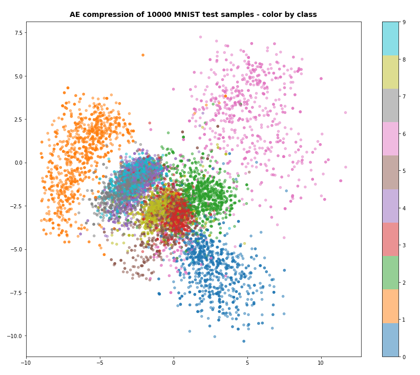
Our Encoder CNN was able to separate the different classes quite well by extraction basic features of the handwritten digits by its Conv2D layers. The test which the AE never had seen before are well separated too:
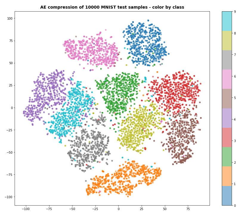
Note that the different position of the clusters on the 2-dim plots are due to transformations and arrangements of t-SNE and have no deeper meaning.
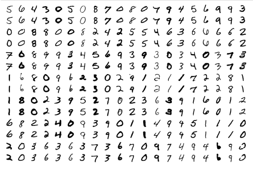
What about the reconstruction quality?
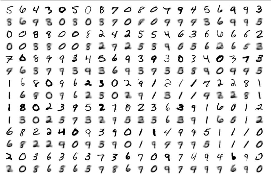
For z_dim = 16 it is almost perfect: Below you see a sequence of rows presenting original images and their reconstructed counterparts for selected MNIST test data, which the AE had not seen before:
The special case of “z_dim = 2”
When we set z_dim = 2 the reconstruction quality of course suffers:
Regarding class related clusters we can directly plot the data distributions in the z-space:
We see a relatively vast spread of data points in clusters for “6”s and “0”s. We also recognize the typical problem zones for “3”s, “5”s, “8”s on one side and for “4”s, “7”s and “9”s on the other side. They are difficult to distinguish with only 2 dimensions.
Conclusion
Autoencoders are simple to set up and work as expected together with Keras and Tensorflow 2.8.
In the next post
Variational Autoencoder with Tensorflow – III – problems with the KL loss and eager execution
we shall, however, see that VAEs and their KL loss may lead to severe problems.
Ceterum censeo: The worst living fascist and war criminal today, who must be isolated, denazified and imprisoned, is the Putler.