
In the last posts of this series
KMeans as a classifier for the WIFI and MNIST datasets – I – Cluster analysis of the WIFI example
KMeans as a classifier for the WIFI and MNIST datasets – II – PCA in combination with KMeans for the WIFI-example
KMeans as a classifier for the WIFI and MNIST datasets – III – KMeans as a classifier for the WIFI-example
we applied the KMeans algorithm to perform a cluster analysis of the WIFI dataset of the UCI Irvine. The results gave us insights into the spatial grouping and the separability of the data samples in their 7-dimensional feature space. An additional PCA analysis helped to understand why projections of the data into some selected 2-dimensional sub-spaces of the feature space revealed the four or five dominant clusters very well. In the third post I discussed a simple method to transform KMeans into a classifier. In the WIFI case a set of 9 to 11 clusters provided a good resolution of the data distribution and we reached a convincing classifier accuracy.
What we have not done, yet, is to transform and project the WIFI data into the coordinate system of the most important main components and afterward apply clustering by the help of KMeans. We know already that three primary components fit the data very well and give us around 90% of the “explained variance“. See the second post for these basic PCA results. We, therefore, expect comparably accurate prediction results of a cluster classifier for the PCA transformed data as the accuracy values given in the last post. For 500 test samples after a KMeans fit of 1500 training samples in the original feature space we found a prediction accuracy of around 98%.
In this post we first perform a PCA analysis for three primary components of the WIFI data distribution and then transform the vectors of 1500 randomly selected training samples to the 3-dimensional main component space. Then we apply KMeans onto the data in the reduced vector space and establish a classifier predictor based on the methods described in the last article. Eventually, we check the accuracy and display the resulting confusion matrix for the 500 test samples.
As a side-step for readers who look for real world use cases regarding signals I want to mention an article in “Nature”, which I found today via a newspaper podcast. There neural firing rates of a brain region, i.e. some very special signals, were used to enable an ALS patient to select letters from presented sequences and form statements – by his “thoughts”. This looks like an environment where Machine Learning really could contribute more in the future.
KMeans as a classifier on the PCA transformed WIFI data
Below I give you the results for the WIFI data transformed and projected to the most important three primary components and 11 clusters:
Results for 1500 training samples
Confusion matrix for training data - 11 clusters, 3 PCA components
A confusion matrix for the classes according to the clustering
[[374   0   1   0]
 [  0 362  13   0]
 [  4   7 359   5]
 [  1   0   0 374]]

Number of wrongly predicted train samples:  31  :: avg_err =  0.020
So, just from counting wrongly classified examples the average error is measured to be around 2% and the relative accuracy is something like 98%.
And for the test data I got:
Number of wrongly predicted test samples: 6 :: avg_err = 0.012
This gives us the following confusion matrix:
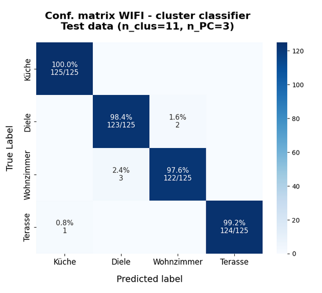
This actually proves that our assumption about combining a PCA transformation with a KMeans classifier was correct. The reduction of the dimensionality of the problem did not affect the prediction accuracy very much.
Just for completeness the data for only 2 primary components:
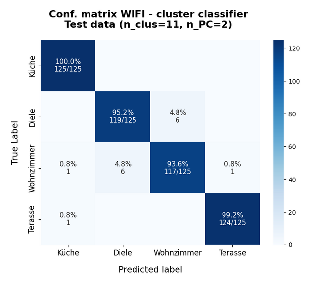
The accuracy of around 97% is still convincing. The reason is that the two most important primary components already deliver around 85% of the “explained variance”.
Why is the Wifi-example not so boring as one may think?
A reader wrote me that he finds the WIFI example too simple and boring. OK, but … The principles and methods remain the same when more complex data are analyzed for clusters. Especially in the case of binary classification. But are there interesting real world use cases for other types of signals? Oh, yes. I just want to refer to an interesting example which I read about this morning.
The WIFI example works with samples which describe 7 signals. Now, imagine that such signals come from a sensor implant measuring electric potentials of a human brain and that we do not analyze for the location of rooms but for the selection of letters by “Yes/No” decision-“imaginations” – made by a human who was trained via frequency based audio-feedback for the brain regions covered by the implants. Science fiction? No, reality. And of huge help for ALS patients. See
Chaudhary, U., Vlachos, I., Zimmermann, J.B. et al. Spelling interface using intracortical signals in a completely locked-in patient enabled via auditory neurofeedback training. Nat Commun 13, 1236 (2022). https://doi.org/10.1038/s41467-022-28859-8
and
https://www.nature.com/articles/s41467-022-28859-8
There, signals were measured from two implant arrays with 64 electrodes. OK, these are somewhat more signals than just 7. But if I understood the text correctly not all channels were used or useful. Just a few. Reminds us of PCA? In addition the time structure of the signal (firing rates) are important – but these are just different signal characteristics. And we have different labels. But, at least in principle, we speak of nothing else than pattern detection based on signal values.
I only had a brief look into the supplementary data of the experiment (an Excel file) and I am not at all familiar with the the experimental setup – but from reading my impression was that just threshold values for the firing rate of some channels were used to distinguish “Yes” from “No”. Maybe we could do a bit better with AI (PCA and classifying according to multidimensional pattern analysis)? Does this look like an interesting use case?
Conclusion
In the case of the WIFI example KMeans can be used as an efficient classifier for samples in a feature space which describes characteristics of multiple signal sources. We have seen that the basic concept also works when we apply KMeans after a PCA based transformation to the most important primary components.
The question is: Does this work equally well for other data sets? The answer depends upon the accuracy by which clusters reside completely within regions of the feature space filled by samples of a specific label.
A data set whose samples show grouping in a multidimensional feature space and appear relatively well separable by their labels is the MNIST data set. In the next post of this series we shall therefore try and apply a clustering algorithm to the MNIST data ensemble.
Stay tuned …
Ceterum censeo: The worst fascist today who must be isolated and denazified is the Putler.