Last week I stared preparing posts for my new blog on Machine Learning topics (see the blog-roll). During my studies last week I came across a scientific publication which covers an interesting topic for ML enthusiasts, namely the question what kind of statistical distributions we may have to deal with when working with data of natural objects and their properties.
The reference is:
S. A. FRANK, 2009, “The common patterns of nature”, Journal of Evolutionary Biology, Wiley Online Library Link to published article
I strongly recommend to read this publication.
It explains statistical large-scale patterns in nature as limiting distributions. Limiting distributions result from an aggregation of the results of numerous small scale processes (neutral processes) which fulfill constraints on the preservation of certain pieces of information. Such processes will damp out other fluctuations during sampling. The general mathematical approach to limiting distributions is based on entropy maximization under constraints. Constraints are mathematically included via Lagrangian multipliers. Both are relatively familiar concepts. The author explains which patterns result from which basic neutral processes.
However, the article also discusses an intimate relation between aggregation and convolutions. The author furthermore presents an related interesting analysis based on Fourier components and respective damping. For me this part was eye-opening.
The central limit theorem is explained for cases where a finite variance is preserved as the main information. But the author shows that Gaussian patterns are not the only patterns we may directly or indirectly find in the data of natural objects. To get a solid basis from a spectral point of view he extends his Fourier analysis to the occurrence of infinite variances and consequences for other spectral moments. Besides explaining (truncated) power law distributions he discusses aspects of extreme value distributions.
All in all the article provides very clear ideas and solid arguments why certain statistical patterns govern common distributions of natural objects’ properties. As ML people we should be aware of such distributions and their mathematical properties.
we have studied the transformation of an ellipse by a shear operation. The coordinates of points on an ellipse and the components of respective position vectors fulfill a quadratic equation (quadratic form):
The superscript “T” symbolizes the transposition operation. The symmetric (2×2)-matrix \( \pmb{\operatorname{A}}_q^O \) defines the original, unsheared ellipse. The suffix “q” indicates the quadratic form. I have shown how the shear parameter λS impacts the coefficients of a corresponding (2×2)-matrix \(\pmb{\operatorname{A}}_q^S \) that defines the sheared ellipse.
What I have not done in the last post is to show how our matrix \(\pmb{\operatorname{A}}_q^S \) is related to a shear matrix \(\pmb{\operatorname{M}}_{sh} \) (see the first post), which describes the effect of the shear on the vectors \( \left(\,x_o,\, y_o\,\right)^T \). I am going to discuss this below. The given matrix relations will also be valid for general n-dimensional ellipsoids.
Matrix relations as discussed below are helpful to accelerate numerical calculations as Numpy (in cooperation with libraries for your OS) provides highly optimized modules for matrix operations. n-dimensional ellipsoids furthermore characterize hyper-surfaces of multivariate normal distributions which appear in certain areas of Machine Learning and respective data.
Matrix describing a centered n-dimensional ellipsoid
We consider n-dimensional and centered ellipsoids whose symmetry centers coincide with the origin of the Euclidean coordinate system [ECS] we work with. A position vector \(\left(\,x_1^o,\, x_2^o\, \cdots x_n^o \right)^T \)
is a vector drawn from the origin to a point on the ellipsoid’s hyper-surface. Note that a general vector of a vector space has no reference to a coordinate system’s origin. Therefore the distinction. A general ellipsoid is defined by a quadratic form in the components of its position vectors. The quadratic form is equivalent to the following matrix equation
where \(\pmb{\operatorname{A}}_{qn}^O \) now represents a symmetric (nxn)-matrix. The “\( \circ \)” symbolizes a matrix product.
Note: A coefficient \( \delta \gt 0 \) which we have used in previous posts on the right side of the equation can be included in the coefficient values of the matrix).
Note that the equations above define an ellipsoid up to a translation vector. This is reflected in the fact that the above equation does not create any linear terms.
Quadratic forms not only define ellipsoids. For an ellipsoid we have to assume that the determinant of\(\pmb{\operatorname{A}}_{qn}^O \) is > 0 and that the matrix is invertible:
Note that you could choose an ECS in which the ellipsoid’s principal axes would align with the ECS’s coordinate axes. Such a choice would correspond to a PCA-transformation of the vector data. \(\pmb{\operatorname{A}}_{qn}^O \) would then become diagonal. This corresponds to the fact that a symmetric matrix always has an eigenvalue-decomposition.
Equation of the quadratic form for the sheared ellipsoid
In the first post of this series I have defined a (invertible) shear matrix as a unipotent matrix \( \pmb{\operatorname{M}}_{sh} \) with all coefficients of the lower triangular part, off the diagonal, being equal to 0.0 and all elements on the diagonal being equal to 1:
So an inverse matrix \( \pmb{\operatorname{M}}_{sh}^{-1} \) exists. Shearing our original ellipse (with position vectors \( \pmb{x_o} \)) leads to new vectors \( \pmb{x_S} \):
Σ is a diagonal (nxm)-matrix with singular values. The column-vectors of U and V are orthogonal singular vectors. Geometrically, U and V can be interpreted s rotational operations.
Therefore, we can decompose a (nxn) upper triangular shear-matrix into two orthonormal (nxn)-matrices U and V plus a diagonal matrix Σ :
This gives us an alternative form to define the inverse shear matrix. Note that the order of the matrices in the matrix products is essential.
An example for the case of a sheared ellipse
We use the example of a sheared ellipse discussed in the last post to verify the results above numerically for a 2-dim case. To write a respective Python/Numpy-program is simple. I will just give you my numerical results below.
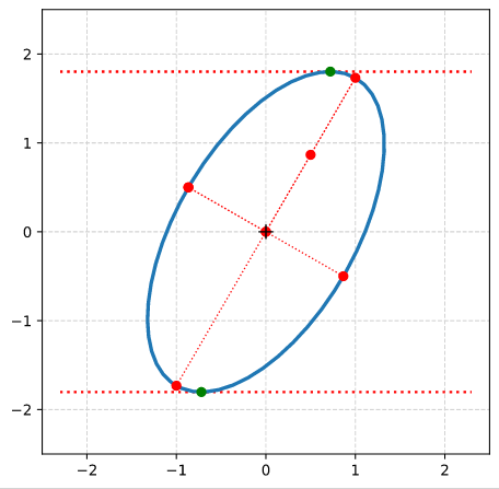
We have used an ellipse with the longer and shorter primary axes having values a = 2 and b = 1, respectively. The ellipse was rotated by 60° against the ECS-axes.
The respective (2×2)-matrix \( \pmb{\operatorname{A}}_q^O \) had the following coefficients
We have shown how a shear matrix \( \pmb{\operatorname{M}}_{sh} \) transforms the matrix \(\pmb{\operatorname{A}}_{qn}^O \) which defines an un-sheared n-dimensional ellipsoid into a matrix \(\pmb{\operatorname{A}}_{qn}^S \) defining its sheared counterpart. We have also had a glimpse on a SVD decomposition of a shear matrix. The results will enable us in the next post to apply shear operations on a concrete example of a 3-dimensional ellipsoid.
Die neue Web-Seite bzw. App der Bahn hielt heute eine weitere Überraschung für uns bereit: Im unseren Kundenaccounts bei der Bahn waren im Gegensatz zur alten Site weder Bahncard noch Bahnbonuspunkte zu finden. Dabei erwies sich das Verhalten von App und Web-Seite (Browser) als unterschiedlich:
Für meine Person wurde die Bahncard in der App angezeigt, in der Webseite jedoch nicht. Ein Versuch, die Daten der Karte per PIN zu übertragen scheiterte mit einer permanenten Fehlermeldung:
“Ihr Konto konnte nicht übertragen werden. Bitte versuchen Sie es später noch einmal. “
Im Falle meiner Frau wurde die Bahncard weder in der App noch im Account auf der neuen Web-Site angezeigt. Auch bei ihr scheiterte der Versuch der Datenübertragung vom Bahnbonus-Account.
Das ist ärgerlich, wenn man die Bonuspunkte für eine geplante Reise verwenden will.
Lösung
Die nicht zugelassene Datenübernahme war in unserem Fall auf etwas unterschiedliche Schreibweisen der Namen zurückzuführen. Hier spielen einerseits Umlaute eine Rolle (die man in früheren Zeiten ggf. zur Erzielung einer Konsistenz mit Daten auf anderen Karten) ausgeschrieben hat (z.B. “ue” statt “ü”). Zu beachten sind auch Umlaute anderer Sprachen als Deutsch. Von Bedeutung ist ferner die Anzahl der angegebenen Vornamen. Das kann man als User nur schwer bereinigen, da unklar ist, welcher Account die führenden Angaben enthält. Ich bin mir im nachhinein auch nicht sicher, ob nach der Umstellung ein separater Login in den Bahnbonus-Account überhaupt noch möglich war.
Geholfen hat uns schließlich eine sehr freundliche Dame des telefonischen Bahnbonus-Services. Tel.-Nummer: 0049 (0)30 2970. Man kommt da mit relativ kurzer Wartezeit durch. Sie konnte die Bahnbonus-Konten und zugehörige Informationen mit dem Bahnkunden-Konto zusammenfügen. Zumindest die Bahnbonus-Punkte tauchen nun ordnungsgemäß auf. In der Smartphone-Apps erscheinen inzwischen auch die Bahncards. Allerdings noch nicht im Bahnkunden-Konto, wenn dies über die neue Webseite im Browser aufgerufen wird.
Diesbzgl. wurden wir auf evtl. folgende Updates der Seiten vertröstet. “Das könne etwas dauern …”. Na ja ….
Bewertung
Bei der Umstellung der Systeme hätten die Entwickler die bisherigen Account-Verknüpfungen von Bahn- und Bahnbonus-Kunden analysieren können und müssen. Die Zuordnung funktionierte ja in der Vergangenheit einwandfrei. Problematische Datensätze hätten vor dem Go Live bewertet und ggf. konsolidiert werden müssen. Zur Not unter Nutzung der Betroffenen. Zumindest Hinweise im Internet wären notwendig gewesen. Generell stellt sich die Frage, wieso man in der Vergangenheit überhaupt mit so vielen verteilten Datensätzen bei der Bahn und Sub-Gesellschaften gearbeitet hat. Bahnkunde, Bahnbonus-Kunde, Bahnkartenbesitzer, …. Seufz.
So, wie sich die Umstellung der Webseiten und die misslungene Zusammenführung der Daten bei der Ban und ihren Sub-Gesellschaften präsentierte, hinterließ das bei uns als regelmäßigen Bahnkunden jedenfalls einen schlechten Eindruck.
Heute früh wollte ich am Linux-PC eine Reise mit der Bahn planen. Dazu rief ich die Seite im Firefox auf. Leider wurde die Bahn-Seite nicht vollständig geladen. Ein Arbeiten war nicht möglich. Das Gleiche unter Chromium und Opera.
Ein Login war zwar möglich, aber auch die dann folgende Seite erlaubte keinerlei Aktion.
Unter Chromium zeigte sich, dass eine Web-Ressource wegen fehlender Autorisierung nicht ansprechbar war.
Neue Web-Präsenz der Bahn
Anfang letzte Woche funktionierte noch alles. Das aktuelle Layout der nur teilweise anzeigten Seite kam mir auch seltsam vor. Eine kurze Suche im Internet zeigte, dass die Bahn ihre Web-Präsenz vollständig hat neu entwickeln lassen. Die neue Web-Präsenz ging zwischenzeitlich live. Neugierig geworden probierte ich einen Aufruf auf einem Win10-System. Identische Probleme unter Chrome und Opera wie unter Linux. Im dortigen Firefox lief die Bahn-Seite aber unter Windows.
Lösung
Durch das Verhalten von Firefox auf dem Win10-Laptop neugierig geworden experimentierte ich ein wenig herum. Am Schluss war die Lösung einfach:
Man muss Cookies und Website-Daten (für bahn.de) sowie alle entsprechenden Daten im Cache der Browser löschen. Und zwar vollständig. Dies erfordert bei Chrome, Chromium und Opera auch eine Einstellung des Zeitraums für den die Löschung vorgenommen werden soll.
Vermutlich ruft die neue Web-Präsenz alte Cookies/Website-Infos (mit falschen Autorisierungsdaten für bestimmte Web-Ressourcen) auf. Das hätten die Entwickler nach meinem Gefühl bei Tests erkennen und abfangen können. Ein Hinweis an neue Benutzer wäre hilfreich. (Der FF unter Win10 war so eingestellt, dass bei dessen Schließung Cache und Cookies automatisch beseitigt wurden. Deswegen tauchte das Problem dort nicht auf.)
Post III focused on the shearing of a circle, which was centered in the Euclidean coordinate system [ECS] we worked with. The shear operation resulted in an ellipse with an inclination against the coordinate axes of our ECS. This was interesting regarding four points:
A circle, which is centered in a chosen ECS, exhibits a continuous rotational symmetry (isotropy). This obviously allows for a decomposition of a shear operation into a sequence of two affine operations in the chosen ECS: a scaling operation (with different factors along the coordinate axes) followed by a rotation (or the other way round). Equivalently: We could switch to another specific ECS which is already rotated by a proper angle against our originally chosen ECS and just perform a scaling operation there. The rotation angle is determined by the shear parameter λ. This seems to stand in some contrast to the shearing of figures with only discrete rotational symmetries: We saw for rectangles and cubes that an additional rotation was required to replace the shear operation by a sequence of scaling and rotation operations.
Points (x, y) of circles and ellipses are described by quadratic forms in two dimensions (with some real coefficients α, β, γ, δ):
\[
\alpha \,x^2 \, + \, \beta \, x \, y \, + \, \gamma \, y^2 \:=\: \delta
\]
Quadratic forms play a general role in the mathematical description of cone-sections. (Ellipses are the results of specific cone-sections.)
Ellipses also result from projections of multi-dimensional ellipsoids onto two-dimensional coordinate planes. Multi-dimensional ellipsoids are described by quadratic forms in an ECS covering the ℝn.
Hyper-surfaces for constant probability density values of multivariate normal vector distributions form multi-dimensional ellipsoids. Here we have a link to Machine Learning where key properties of certain objects are often ruled by Gaussian distributions.
From the first point we may expect that a shear operation applied to a multi-dimensional sphere will result in a multi-dimensional ellipsoid – and that such an operation could be replaced by scaling the original sphere (with different factors along n coordinate axes of a n-dimensional ECS) followed by a rotation (or vice versa). We will explicitly investigate this for a 3-dimensional sphere in the next post.
If our assumption were true we would get a first glimpse of the fact that a general multivariate standard distribution can be created by applying a sequence of distinct affine (i.e. linear) operations to a spherical probability distribution. This is discussed in detail in another post-series in this blog.
What is a bit confusing at the moment is that a replacement of a shear operation by simpler affine operations in general seems to require at least two rotations, but only one when we work with centered isotropic bodies. We come back to this point when we discuss the decomposition of a shear matrix by the so called SVD-procedure.
In the previous post of this series we have used the radius of the circle and the shearing parameter λ to derive analytical expressions for the coordinates of special points with extremal values on our ellipse
Points with maximal and minimal y-coordinate values.
Points with a maximal or minimal distance to the symmetry center of the ellipse. I.e. the end-points of the principal diameters of the ellipse.
From the fact that shearing does not change extremal values along the axis perpendicular to the sharing direction we could easily determine the lengths of the ellipse’s principal axes and the inclination angle of the longer axis with the x-axis of our Euclidean coordinate system [ECS].
What do we have in addition? In another mini-series on ellipses
I have meanwhile described how the geometry of an ellipse is related to its quadratic form and respective coefficients of a symmetric matrix. I call this matrix Aq. It forces the components of position vectors to fulfill an equation based on a quadratic polynomial. Furthermore Aq‘s eigenvalues and eigenvectors define the lengths of the ellipse’s principal axes and their inclination to the axes of our chosen ECS. The matrix coefficients in addition allow us to determine the coordinates of the points with extremal y-values on an ellipse. We will use these results later in the present post.
Objectives of this post: Shearing of a centered, rotated ellipse
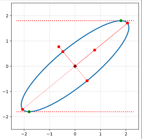
In this post I want to show that shearing a given centered, but rotated original ellipse EO results in another ellipse ES with a different inclination angle and different sizes of the principal axes.
In addition we will derive the relations of the shearing parameter λS with the coefficients of the symmetric matrix \(\pmb{\operatorname{A}}_q^S \) that defines ES. I also provide formulas for the dependence of ES‘s geometrical properties on the shear parameter λS.
There are two basic prerequisites:
We must show that the application of a shear transformation to the variables of the quadratic form which describes an ellipse EO results in another proper quadratic form and a related matrix \(\pmb{\operatorname{A}}_q^S \).
The coefficients of the resulting quadratic form and of \(\pmb{\operatorname{A}}_q^S \) must fulfill a mathematical criterion for an ellipse.
We expect point 1 to be valid because a shear operation is just a linear operation.
To get some exercise we approach our goals by first looking at the simple case of shearing an axis-parallel ellipse before extending our considerations to general ellipses with an inclination angle against the coordinate axes of our chosen ECS.