
I continue with my series on Variational Autoencoders [VAEs] and related methods to control the KL-loss.
Variational Autoencoder with Tensorflow 2.8 – I – some basics
Variational Autoencoder with Tensorflow 2.8 – II – an Autoencoder with binary-crossentropy loss
Variational Autoencoder with Tensorflow 2.8 – III – problems with the KL loss and eager execution
Variational Autoencoder with Tensorflow 2.8 – IV – simple rules to avoid problems with eager execution
Variational Autoencoder with Tensorflow 2.8 – V – a customized Encoder layer for the KL loss
Variational Autoencoder with Tensorflow 2.8 – VI – KL loss via tensor transfer and multiple output
Variational Autoencoder with Tensorflow 2.8 – VII – KL loss via model.add_loss()
Variational Autoencoder with Tensorflow 2.8 – VIII – TF 2 GradientTape(), KL loss and metrics
Variational Autoencoder with Tensorflow 2.8 – IX – taming Celeb A by resizing the images and using a generator
Variational Autoencoder with Tensorflow 2.8 – X – VAE application to CelebA images
Variational Autoencoder with Tensorflow 2.8 – XI – image creation by a VAE trained on CelebA
After having successfully trained a VAE with CelebA data, we have shown that our VAE can afterward create images with human-like looking faces from statistically selected data points (z-points) in its latent space. We still have to analyze the confinement of the z-point distribution due to the KL-loss a bit in more depth. But before we turn to this topic I want to briefly discuss an option to reduce the VRAM requirements of the VAE’s Encoder.
Limited VRAM – a problem for ML training runs on older graphics cards
In my opinion exploring the field of Machine Learning on a PC should not be limited to people who can afford a state of the art graphics card with a lot of VRAM. One could use Google’s Colab – but … I do not want to go into tax and personal data politics here. I really miss an EU-wide platform that offers services like Google Colab.
Anyway, a reduction of VRAM consumption may be decisive to be able to perform training runs for CNN-based VAEs on older graphic cards . Not only concerning VRAM limits but also regarding computational time: The less VRAM the weight parameters of our VAE models require the bigger we can size the batches the GPU operates on and the more CPU time we may potentially save. At least in principle. Therefore, we should consider the amount of trainable parameters of a neural network model and reduce them if possible.
The number of parameters depends heavily on the connections to the mu and logvar-layer of the Encoder
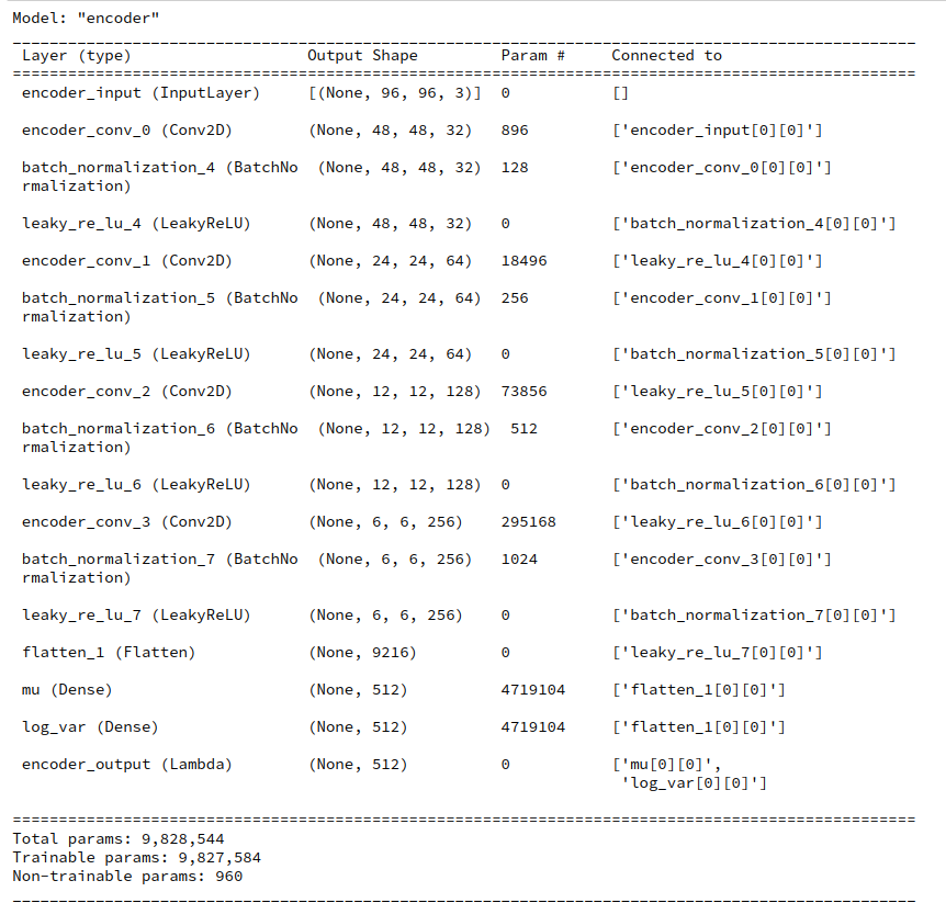
When you print out the layer structure and related parameters of a VAE (see below) you will find that the Encoder requires more parameters than the Decoder. Around twice as many. A closer look reveals:
It is the transition from the convolutional part of the Encoder to its Dense layers for mu and logvar which plays an important role for the number of weight parameters.
For a layer structure comprising 4 Conv2D layers, related filters=(32,64,128,256) and an input image size of (96,96,3) pixels we arrive at a Flatten-layer of 9216 neurons at the end of the convolutional part of the Encoder. For z_dim = 512 the direct connections from the Flatten-layer to both the mu- and logvar-layers lead to more the 9.4 million (float32) parameters for the Encoder. This is the absolutely dominant part of all required 9.83 million parameters of the Encoder. In contrast the Decoder part requires a total of 5.1 million parameters, only.
Encoder
Decoder
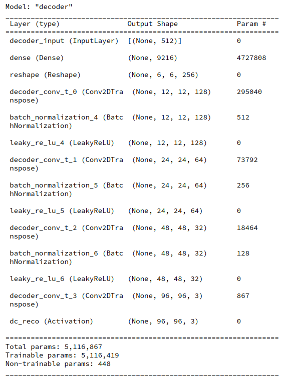
This is due to the fact that the flattened layer supplies input to two connected layers before output is created by yet another layer. In the Decoder, instead, only one layer, namely the input layer is connected to the flattened layer ahead of the first Conv2DTranspose layer.
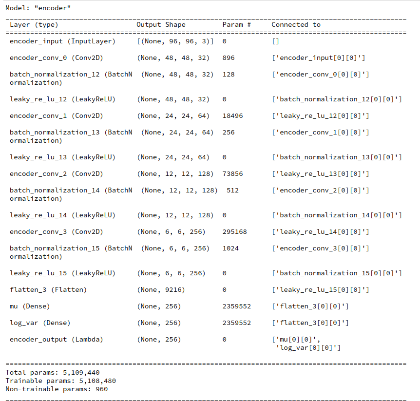
In the case of z_dim=256 we arrive at around half of the parameters, i.e. 4.9 million parameters for the Encoder and around 2.76 million for the Decoder.
It is obvious that the existence of two layers for the variational parameters inside the Encoder is the source of the high parameter number on the Encoder side.
Would a reduction of convolutional layers help to reduce the weight parameters?
A reduction of Conv2D-layers in the Encoder would of course reduce the parameters for the weights between the convolutional layers. But turning to only three convolutional layers whilst keeping up a stride value of stride=2 for all filters would raise the already dominant number of parameters after the flattened layer by a factor of 4!
So, one has to work with a delicate balance between the number of convolutional layers and the eventual number of maps at the innermost layer and the size of these maps. They determine the number of neurons and related weights on the flattening layer:
From the perspective of a low total number of parameters you should consider higher stride values when reducing the number of Conv2D-layers.
On the other hand side using more than 4 convolutional layers would reduce the resolution of the maps of the innermost Conv2D layer below a usable threshold for reasonable mu and logvar values.
Off topic remark: All in all it seems to be reasonable also to think about ResNets of low depth instead of plain CNNs to keep weight numbers under control.
An intermediate dense layer ahead of the mu- and logvar-layers of the Encoder?
The reader who followed the posts in this series may have looked at the recipe which F. Chollet has discussed in his Keras documentation on VAEs. See:
https://keras.io/ examples/ generative/vae/.
There is an element in Chollet’s Encoderstructure which one easily can overlook at first sight. In his example for the MNIST dataset Chollet adds an intermediate Dense layer between the Flatten-layer and the layers for mu and logvar.
...
x = layers.Flatten()(x)
x = layers.Dense(16, activation="relu")(x)
z_mean = layers.Dense(latent_dim, name="z_mean")(x)
z_log_var = layers.Dense(latent_dim, name="z_log_var")(x)
...
In the special case of MNIST an intermediate layer seems appropriate for bridging the gap between an input dimension of 784 to z_dim = 2. You do not expect major problems to arise from such a measure.
But: This intermediate layer introduced by Chollet also has the advantage of reducing the total number of trainable parameters substantially.
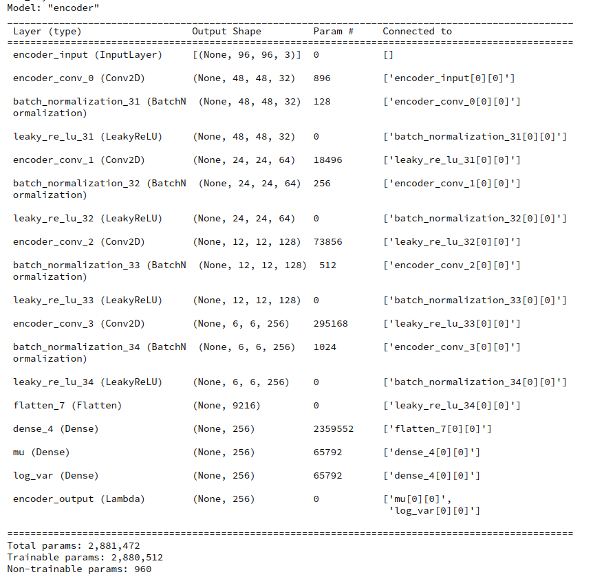
We could try something similar for our network. But here we have to be a bit more careful as we work in a latent space of much higher dimensions, typically with z_dim >= 256. Here we are in dilemma as we want to keep the intermediate dimension relatively high for using as much information as possible coming from the maps of the last Conv2D-layers. A fair compromise seems to be to use at least the dimension of the mu and varlog-layers, namely z_dim.
For z_dim=256 an additional Dense layer of the same size would reduce the total number of Encoder parameters from 5.11 million to 2.88 million.
If we took the dimension of the intermediate layer to be 384 we would still go down with the total Encoder parameters to 4.13 million. So an additional Dense layer really saves us some VRAM.
Images constructed by a VAE model with an additional Dense layer in the Encoder
Will an additional dense layer have a negative impact on our VAE’s ability to create images from randomly chosen z-points in the latent space?
Let us try it out. To include an option for an additional Dense layer in the Encoder related part of our class “MyVariationalAutoencoder()” is a pretty simple task. I leave this to the reader. Note that if we choose the dimension of the additional Dense layer to be exactly z_dim there is no need to change the reconstruction logic and layer structure of the Decoder. Also for other choices for the size of the Dense layer I would refrain from changing the Decoder.
I used z_dim=256 for the extra layer’s size. Then I repeated the experiments described in my last post. Some results for random z-points picked from a normal distribution in all coordinates are shown below:
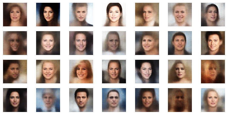
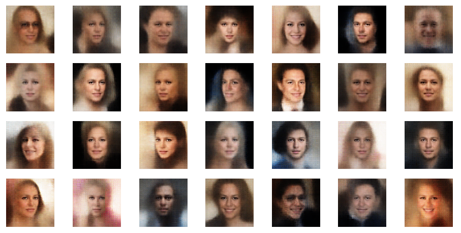
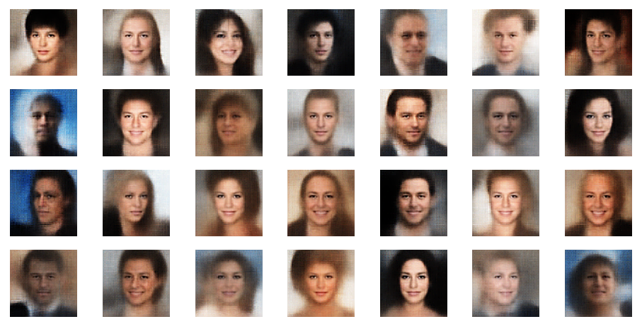
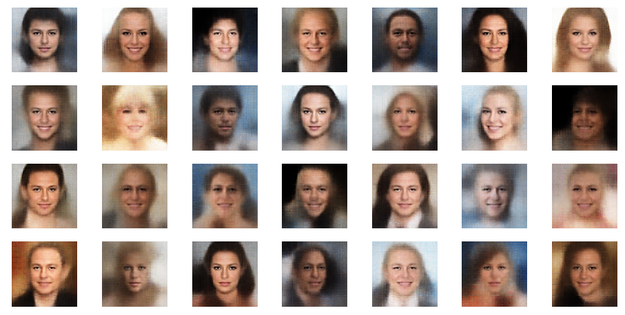
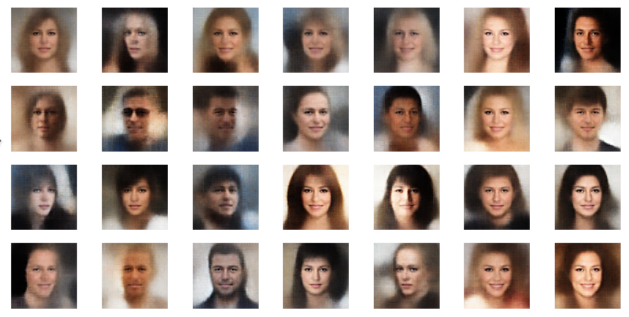
So we see that from the generative point of view an extra Dense layer does not hurt too much.
What have we gained?
First and foremost:
We found a simple method to reduce the VRAM consumption of the Encoder.
But I have to admit that this method did NOT save any GPU time during training as long as I kept the size of image batches equally big as before (128). The reason is:
Due to the extra layer more matrix operations have to be performed than before, although some of matrixes becae smaller. On my old graphics card a full epoch with 170,000 (96×96) images takes around 120 secs – with or without an extra Encoder layer. Unfortunately, increasing the size of the batches the DataImageGenerator feeds into the GPU from 128 images to 256 did not change the required GPU time very much. More tests showed that a size of 128 already gave me an optimal turnaround time per epoch on my old graphics card (960 GTX).
Conclusion
An extra intermediate Dense layer between the Flatten-layer and the mu- and logvar-layers of the Encoder can help us to save some VRAM during the training of a VAE. Such a layer does not lead to a visible reduction of the quality of VAE-generated images from randomly selected points in the latent-space.
In the next post of this series
Variational Autoencoder with Tensorflow 2.8 – XIII – Does a VAE with tiny KL-loss behave like an AE? And if so, why?
we will compare a VAE with only a tiny contribution of KL-loss to the total loss with a corresponding AE. We shall investigate their similarity regarding their z-point distributions. This will give us a solid basis to investigate the impact of higher KL-loss values on the latent space in more detail afterwards.