In my first article in this series on local and remote connections to the Spice console of a KVM/Qemu virtual machine [VM] I have given you an overview over some major options. See the central drawing in
In this post we explore a part of the drawing’s left side – namely a local connection with the remote-viewer client over a network-port and the “lo”-device. Local means that we access the Spice console with a Spice client in a desktop session on the KVM/Qemu host.
You can find some basic information on “remote-viewer” here.
Note: “remote-viewer” supports VNC, too, but we ignore this ability in this series.
A local scenario with remote-viewer on a KVM/Qemu host corresponds to desktop virtualization – though done with a remote tool. Such an approach can become a bit improper, because setting up ports for potential remote network connections always has security implications. This is one of the reasons why I actually want to discuss two different local access methods which can be realized with remote-viewer:
- Method 1: Access via a network port (TCP socket). This standard method is well documented on the Internet both regarding the VM’s setup (e.g. with virt-manager) and the usage of remote-viewer (see the man pages). The network based scenario is also depicted in my drawing.
- Method 2: Access via a local Unix socket. This method is not documented so well – neither regarding the VM’s setup (e.g. with virt-manager) and not at all by the man pages for remote-viewer.
You may complain now that I never indicated anything in the above drawing about a pure Unix socket! Well, at the time of writing the first article I did not even know that remote-viewer worked over a pure Unix socket and how one can configure the VM for a Unix socket. I will discuss the more common “Method 1” in this present article first. “Method 2” will be the subject of the next post – and then I will provide an update of the drawing. Talking about sockets: When you think a bit about it – Unix sockets must already be an ingredient of the local interaction of libvirt-tools with qemu, too, ….
Below I will discuss a set up for “Method 1” which is totally insecure. But it can be realized in a very simple way and is directly supported by virt-manager for the VM setup. Thus, it will give us a first working example without major efforts for creating TLS certificates. But, you are/were warned:
Disclaimer:
The test-configurations I discuss in this and the next articles of this series may lead to major security risks. Such configurations should NOT be used in productive multi-user and/or network environments without carefully crafted protection methods (outside the qemu-configuration) – as local firewall protection, system policies, etc. I take no responsibility whatever for an improper usage of the ideas presented in this article
series.
Assumptions for test scenarios
- The KVM/Qemu host in this article series is an Opensuse Leap 15.2 host. Most of the prescriptions discussed may work with some minor modifications also on other Linux distributions. But you must look up documentations and manuals …
- I assume that you already have set up a KVM/Qemu based test-VM with virsh or virt-manager. Let us call the VM “debianx“. Actually, it is a Kali system in my case. (Most of the discussed measures will work on guests with a Debian OS, too.)
- On our Opensuse KVM host we find a XML-definition file “debianx.xml” for a libvirt domain (i.e. a VM) below the directory “/etc/libvirt/qemu/“, i.e. “/etc/libvirt/qemu/debianx.xml”. It has a typical XML structure and can be edited directly if required.
- The KVM host itself has a FQDN of “MySRV.mydomain.de“. (MySRV is partiall writtenin big letters to remind you that you have to replace it by your own domain.
- The user on the KVM host, who invokes remote-viewer to access the VM, has a name “uvma“. We will later add him to a group “libvirt” which gets access rights to libvirt tools. We shall also work with a different user “uvmb” who is a member of the group “users”, only. Both users work on a graphical desktop on the KVM/Qemu host (!) – let us say a KDE desktop. These users open one or more Spice client windows on the host’s desktop to display graphical desktops of the KVM/Qemu guest VMs – as if the windows were screens of the VM.
We must carefully distinguish between the (KDE) desktop used by “uvma” on the KVM host and the desktop of the guest VM:
The Spice client windows on the KVM host’s (or later on independent remote systems) desktop present full graphical desktops (Gnome, XFCE, KDE …) of the VM and allow for interactive working with the VM. The desktop used on the host can, of course, be of a different type than the one used on the guest.
I will use this first practical article also
- to have a brief look at two basic configuration files for libvirtd and qemu settings,
- to discuss some basic setup options for a Qemu VM,
- to check the multi-screen ability of remote-viewer
- and to prove the “one-seat” situation for the Spice console.
I restrict my hints regarding the guest configuration to Kali/Debian or Opensuse Leap guest systems on the VM. I provide images for a Kali guest system, only. I do not have time for more …
Make backups
Before you start any experiments you should make a backup of the directories “/etc/libvirt” and “/etc/pki” of your host – and in doubt also of the disk-files (or real partitions) of your existing VMs. You should also experiment with a non-productive test VM, only.
Basic security considerations
(In-) Security is always a bit relative. Let us consider briefly, what we intend to do with respect to “Method 1”:
With the first method we define a network port for unencrypted connections without authentication.
In principle the port can be used by anyone having access to your network or anyone present on your PC. Such a configuration is therefore only reasonable for desktop virtualization
- if you really are alone on your PC
nOtherwise it opens a much too big attack surface. Remember: Anyone being able to use the network port can kick you off your Spice console session seat, remotely, locally and also when you are already logged into the guest OS. And:
All data transfer over any kind of network device (lo, ethernet, virtual devices on the host, …) occurs unencrypted. Other users on your machine (legal users, e.g. active via ssh, or attackers) may with some privilege escalation be able to read it.
Access to the Spice console itself can, however, be restricted to users who know a password. At the end of this article we will add such a simple password to our configuration to get at least some basic protection against kicking you out of a Spice console session.
Preparational step 1: Settings in “/etc/libvirt/qemu.conf” and the integration of Spice with Qemu
As mentioned in the last article, Spice is fully integrated with the Qemu-emulator. So, it will not surprise you that we can modify some general properties of connections to a VM’s Spice console by parameter settings in a configuration file for Qemu. The relevant file in the libvirt-dominated virtualization environment of Opensuse Leap 15.2 is
“/etc/libvirt/qemu.conf“.
Readers of my last article may ask now: Why do we need to configure the Qemu-driver of libvirt at all, when we access the Spice console with remote-viewer directly via Qemu ? I.e., without passing a libvirt-layer? As depicted in the drawing?
Answer: Probably you and me start KVM/Qemu based VMs through “virsh” or “virt-manager“, i.e. libvirt components. Then libvirt drivers which are responsible to start the VMs according to its setting profile must know what we expect from the Qemu emulator. If you worked directly with the qemu-emulator (by calling “/usr/bin/qemu-x86_64”) you would have to specify a lot of options to control the outcome! Some sections below you will find an example. Libvirt-programs only automate this process.
“qemu.conf” allows for general default settings of a variety of qemu-parameters. Some of them can, however, be overwritten by VM-specific settings; see the next section. When you scroll through the file you come to a major section which contains Spice parameters. For an easy beginning of our experiments we set some selected parameters to the following values:
#spice_listen = "0.0.0.0" # just leave it as it is
# ....
spice_tls = 0  # This corresponds to a deactivation of TLS and a INSECURE configuration!
spice_tls_x509_cert_dir = "/etc/pki/libvirt-spice"
# ....
# just leave the next settings as it is - it creates a socket at  "/var/lib/libvirt/qemu/domain-1-debianx/monitor.sock"
#spice_auto_unix_socket = 1
spice_sasl = 0
Our first setting deactivates TLS. This is reasonable as long a we have not created valid TLS server certificates and encryption keys. But we can already define a default directory into which we later place such a certificate and key files. We also deactivate any SASL authentication support for the time being. (Actually, even if you left it at the default value of “1” it would not help you much – as on Opensuse systems a required file “/etc/sasl2/qemu.conf” is missing, yet. As standard SASL encryption methods are insecure today, SASL activation makes sense in combination with TLS only.
General security precautions in “/etc/libvirt/qemu.conf”
Talking about security: On an Opensuse system with activated “apparmor” you could/should set the following parameters in “/etc/libvirt/qemu.conf”:
security_driver = "apparmor"
security_default_confined = 1
to confine VMs.
Note: If “apparmor” is deactivated for some reason you will after these settings not be able to use virt-manager or virsh.
You can check the status of apparmor via “rcapparmor status” or systemctl status apparmor”.
(Off topic: Those interested in process separation should also have a look at cgroup-settings for the VMs. I would not change the basic settings, if you do not know exactly what you are doing. But folks trying to experiment with “virgl3D” may need to add “/dev/dri/renderD128” to the device list for ACLs.)
Preparational step A: A brief look a “/etc/libvirt/libvirtd.conf” – allow a selected standard user to use virt-manger or virsh
As we are within the folder “/etc/libvirt”, we take the chance to very briefly look at another configuration file, which will become more interesting in later articles:
/etc/libvirt/libvirtd.conf
Among other things this file contains a variety of parameters which control the access to libvirt tools via Unix sockets or TCP-sockets – with and without TLS and/or some form of authentication. This is of no direct importance for what we presently are doing with remote-viewer – as we access Spice console directly via qemu, i.e. without a libvirt-layer. However, for convenience reasons you should nevertheless be able to use virt-manager or virsh. If you do not want to work as root all the time you, i.e. he normal user “uvma”, need(s) special access rights to access Unix sockets which are automatically opened by libvirtd. How can this be achieved on an Opensuse Leap system?
You can configure a special user-group (e.g. a group named “libvirt”) to get access to virt-manager. You can do this in a section named “UNIX socket access controls”. The instructions in Opensuse’s documentation on virtualization (see: Connections and authorization and section 9.1.1.1 therein) will help you with this. Afterwards you must of course add your selected and trusted user (here: “uvma”) to the defined group.
Note: The libvirtd-process is nevertheless run by the user “root” and not with the rights of the standard user (here “uvma”). The group just allows for a kind of sudo execution. Note also that the central sockets by which libvirt-clients connect to the libvirtd-daemon are created by systemd.
By the way – who is the user for qemu-processes on an Opensuse Leap system?
On an Opensuse there is a special user “qemu” which is used to run the Qemu-emulator processes for VMs. We also find a related group “qemu”. User and group have special rights regarding aes-keys for potential credential encryption related to a VM. The user and its group also define the access right to special Unix sockets generated directly by the Qemu emulator and not by libvirtd. We shall request such a Unix socket from Qemu in the next article.
On other operative systems you may find a different pre-configured group for libvirt access rights. In addition the standard qemu-user may have a different name. For Debian and derivatives you find related information at the following links:
whats-the-purpose-of-kvm-libvirt-and-libvirt-qemu-groups-in-linux,
install-configure-kvm-debian-10-buster,
libvirt_qemu_kvm_debian .
Preparational step B: Restart libvirtd or reload its configuration after changes to qemu.conf, livirtd.conf or changes to XML-definition files for VMs
Changes of the file “/etc/libvirt/qemu.conf” or “/etc/libvirt/libvird.conf” require that the libvirtd daemon is restarted or forced to reload its configuration. The same is true for any changes of
XML-definition files for VMs located in “/etc/lbvirt/qemu/”. (We will change such files later on). According to the man page sending a SIGHUP signal to the daemon will enforce a reload of the configuration. You can indirectly achieve this by the commands
rclibvirtd reload [on Opensuse systems)
or
systemctl reload libvirtd [any system with systemd]
But: Any libvirt or qemu changes will NOT affect already running VMs. You have to stop them, then restart libvirtd, reload the daemon’s configuration and restart the VMs again.
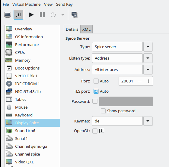
Preparational step C: Configure the VM to use a Spice-console – and some other devices
Ok, let us prepare our VM for “Method 1”. As we are in a libvirt environment we could use virt-manager to perform the required Spice configuration (see the image in the first article) . But we can also directly edit the XML configuration file “/etc/libvirt/qemu/debianx.xml” – assuming that you already have a working configuration for your VM. You need to be root to edit the files directly. See the restrictive access rights of the domain definition files
-rw------- 1 root root 4758 Mar 8 13:33 debianx.xml
By the way: A detailed description of possible parameter settings is provided at https://libvirt.org/formatdomain.html. Search for Spice and qxl …..
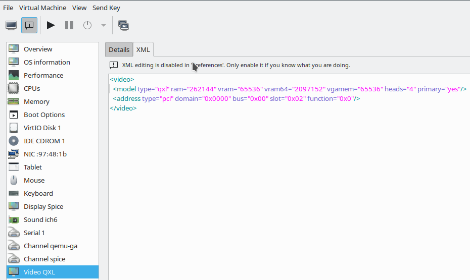
Regarding “Method 1” I use the following settings. The listing below only gives you an excerpt of the XML domain file, but it contains the particularly relevant settings for “graphics” (can be looked upon as a display device) and “video” (an be interpreted as a kind of virtual graphics card):
Excerpts from a libvirt domain definition XML file
   <interface type='network'>
      <mac address='52:54:00:93:38:4c'/>
      <source network='os'/>
      <model type='virtio'/>
      <address type='pci' domain='0x0000' bus='0x00' slot='0x03' function='0x0'/>
    </interface>
   ...
   <graphics type='spice' port='20001' autoport='no' listen='0.0.0.0' keymap='de' >
      <listen type='address' address='0.0.0.0'/>
      <image compression='off'/>
    </graphics>
   ...
    <sound model='ich6'>
      <address type='pci' domain='0x0000' bus='0x00' slot='0x04' function='0x0'/>
    </sound>
    ...
    <video>
      <model type='qxl' ram='262144' vram='65536' vram64='2097152' vgamem='65536' heads='4' primary='yes'/>
      <address type='pci' domain='0x0000' bus='0x00' slot='0x02' function='0x0'/>
    </video>
...
Parameters which affect general qemu-related properties (as e.g. the “listen”-settings) will overwrite the settings in “qemu.conf”. The choice of the PCI slot numbers may be different for your guest.
You see that I defined a network (!) port for the VM by which we can access the Spice console data stream directly. I have changed this port from the default “5900” to “20001”.
You should be aware of the fact that this sets a real network port on the KVM host – i.e. a network stack is invoked when accessing the Spice console. As indicated above we can avoid the superfluous network operations by directly working with a Unix socket (Method 2), but this is the topic of the next forthcoming article.
Regarding network port definitions for a Spice console three rules apply:
- Each of the VMs defined requires its own individual port !
- Firewalls between the client and the VM have to be opened for this port. This includes local firewalls on the VM, on the KVM host (with rules that may apply to virtual bridges, on the client system and on any network
components in between. - A TLS port has later to be configured in addition if you deactivated the “autoport” functionality – as we have done in the example above. I shall describe how to set the TLS port in a forthcoming article.)
The individual port definitions already imply the provision of a URI with port specification when starting remote-viewer (see below).
Let me briefly comment on the QXL-settings:
The QXL configuration shown above allows for 4 so called “heads” (or connectors) of the virtual graphics device. These heads support up to 4 virtual screens, if requested by the Spice-client. Note that the situation is different from real hardware consoles:
The (Spice) client (here remote-viewer) defines the number of screens attached to the VM’s console by a number of Spice client windows opened on the user’s desktop on the KVM host. The dimensions of these Spice client windows determine the dimensional capabilities of the virtual “screens”.
How the virtual screen resolution is handled afterwards may depend on the user’s own desktop resolution (on the KVM host or a remote system) AND the display settings of the VM’s guest system’s own tools for screen management. Today these are typically tools integrated into the guest’s graphical desktop (KDE, Gnome, XFCE) itself. Present Gnome and KDE5 desktops on the VM’s guest Linux system automatically adapt to the virtual display dimensions – i.e. the Spice window dimensions. But a XFCE desktop on the guest may behave differently; see below.
A short note also on the network settings for our test VM:
A virtual machine will normally be associated with a certain type of virtual network. At least if you want to use it for the provision of services or other network or Internet dependent tasks. You can configure virtual networks with virt-manager (menu “edit” >> “connection details”); but you must be root to do this:
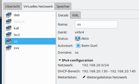
In my case I prefer a separate virtual network for which we need routing on the KVM host. This allows us to configure restrictive firewall rules – e.g, with netfilter on the host. It even allows for the setup of virtual VLANs – a topic which I have extensively covered in other article series in this blog. And when required we just can stop routing on the host.
Guest requirements
Note that the QXL-configuration must also be supported on the VM guest itself: You need a qxl-video-driver there – and it is useful to also have the so called spice-vdagent active (see the my referenced series about a qxl-setup in the last article). On the guest system this requires
- the installation of the “spice-vdagent” package and the activation of the “spice-vdagent.service” (both on Debian/Kali and Opensuse guest systems) ,
- the installation of the packet “xserver-xorg-video-qxl” on a Debian/Kali-guest or “xf86-video-qxl” on an Opensuse guest
Present Debian, Kali or Opensuse operative system on the KVM/Qemu guest VM should afterward automatically recognize the QXL-video-device and load the correct driver (via systemd/udev).
Regarding the (virtual) network device on the VM itself you must use the guest system’s tools for the configuration of NICs and of routes.
Preparational step D: Starting the VM – and “Where do I find logs for my VM”?
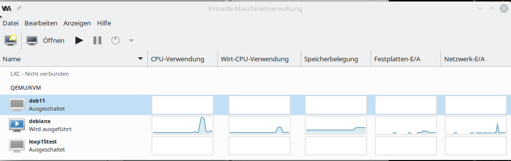
I assume that you as user “uvma” are logged in to a graphical desktop session on your KVM host “MySRV”. If you are not
yet a member of the libvirt-privileged group, you may need to use sudo for the next step. On a terminal window you then enter “virt-manager &”, select our VM “debianx” and boot it.
If you look at the process list of your KVM host you may find something like:
qemu 17662 5.5 6.8 15477660 4486180 ? Sl 18:11 2:29 /usr/bin/qemu-system-x86_64 -machine accel=kvm -name guest=debianx,debug-threads=on -S -object secret,id=masterKey0,format=raw,file=/var/lib/libvirt/qemu/domain-1-debianx/master-key.aes -machine pc-i440fx-2.9,accel=kvm,usb=off,vmport=off,dump-guest-core=off -cpu Skylake-Client -m 8192 -overcommit mem-lock=off -smp 3,sockets=3,cores=1,threads=1 -uuid 789498d2-e025-4f8e-b255-5a3ac0f9c965 -no-user-config -nodefaults -chardev socket,id=charmonitor,fd=33,server,nowait -mon chardev=charmonitor,id=monitor,mode=control -rtc base=utc,driftfix=slew -global kvm-pit.lost_tick_policy=delay -no-hpet -no-shutdown -global PIIX4_PM.disable_s3=1 -global PIIX4_PM.disable_s4=1 -boot strict=on -device ich9-usb-ehci1,id=usb,bus=pci.0,addr=0x5.0x7 -device ich9-usb-uhci1,masterbus=usb.0,firstport=0,bus=pci.0,multifunction=on,addr=0x5 -device ich9-usb-uhci2,masterbus=usb.0,firstport=2,bus=pci.0,addr=0x5.0x1 -device ich9-usb-uhci3,masterbus=usb.0,firstport=4,bus=pci.0,addr=0x5.0x2 -device virtio-serial-pci,id=virtio-serial0,bus=pci.0,addr=0x6 -blockdev {"driver":"file","filename":"/virt/debs/debianx.qcow2","node-name":"libvirt-2-storage","cache":{"direct":true,"no-flush":false},"auto-read-only":true,"discard":"unmap"} -blockdev {"node-name":"libvirt-2-format","read-only":false,"cache":{"direct":true,"no-flush":false},"driver":"qcow2","file":"libvirt-2-storage","backing":null} -device virtio-blk-pci,scsi=off,bus=pci.0,addr=0x7,drive=libvirt-2-format,id=virtio-disk0,bootindex=1,write-cache=on -device ide-cd,bus=ide.0,unit=0,id=ide0-0-0 -netdev tap,fd=35,id=hostnet0,vhost=on,vhostfd=36 -device virtio-net-pci,netdev=hostnet0,id=net0,mac=52:54:00:93:38:4c,bus=pci.0,addr=0x3 -chardev pty,id=charserial0 -device isa-serial,chardev=charserial0,id=serial0 -chardev socket,id=charchannel0,fd=37,server,nowait -device virtserialport,bus=virtio-serial0.0,nr=1,chardev=charchannel0,id=channel0,name=org.qemu.guest_agent.0 -chardev spicevmc,id=charchannel1,name=vdagent -device virtserialport,bus=virtio-serial0.0,nr=2,chardev=charchannel1,id=channel1,name=com.redhat.spice.0 -device usb-tablet,id=input0,bus=usb.0,port=1 -spice port=20001,addr=0.0.0.0,disable-ticketing,plaintext-channel=default,image-compression=off,seamless-migration=on -k de -device qxl-vga,id=video0,ram_size=268435456,vram_size=67108864,vram64_size_mb=2048,vgamem_mb=64,max_outputs=4,bus=pci.0,addr=0x2 -device intel-hda,id=sound0,bus=pci.0,addr=0x4 -device hda-duplex,id=sound0-codec0,bus=sound0.0,cad=0 -chardev spicevmc,id=charredir0,name=usbredir -device usb-redir,chardev=charredir0,id=redir0,bus=usb.0,port=2 -chardev spicevmc,id=charredir1,name=usbredir -device usb-redir,chardev=charredir1,id=redir1,bus=usb.0,port=3 -device virtio-balloon-pci,id=balloon0,bus=pci.0,addr=0x8 -object rng-random,id=objrng0,filename=/dev/urandom -device virtio-rng-pci,rng=objrng0,id=rng0,bus=pci.0,addr=0x9 -sandbox on,obsolete=deny,elevateprivileges=deny,spawn=deny,resourcecontrol=deny -msg timestamp=on
You see that the user “qemu” started the qemu-process by calling “/usr/bin/qemu-system-x86_64” and adding a bunch of parameters. You may identify some parameters which stem from the settings in libvirt’s XML definition file for our special the VM (or “domain”).
Afterwards, have a look at connections with
netstat on the host; you should see that something (qemu) listens on the defined Spice port of the VM:
MySRV:/etc/libvirt/qemu # netstat -a -n | grep 20001
tcp        0      0 0.0.0.0:20001           0.0.0.0:*               LISTEN
...
Regarding logs of the VM for error analysis: You will find them in the directory ” /var/log/libvirt/qemu” (on an Opensuse Leap system).
Method 1: Local access to the Spice console with remote-viewer
Now, we are prepared to test a local access to the Spice console with remote-viewer. (As we work via a network port you may still need to open the Spice port on a local firewall – it depends of how you configured your firewall.) The format of the URI we have to specify for remote-viewer is
spice://FQDN_OR_IP:PORT_NR
with
- FQDN_OR_IP: You have to present a host address which can be resolved by DNS or a directly an IP-address.
- PORT_NR: The port for the Spice service – here “20001”.
For our setup this translates to
spice://localhost:20001
and thus the command
remote-viewer spice://localhost:20001
As user “uvma” we enter this command in another terminal window of our graphical desktop on the KVM host :
uvma@MySrv:~> remote-viewer spice://localhost:20001

(remote-viewer:22866): GSpice-WARNING **: 12:43:58.150: Warning no automount-inhibiting implementation available
Just ignore the warning. Then you should get a window with a graphical display of some login-screen on the VM. Details depend of course on the configuration of your VM’s operative system. In my case, I get the “gdm3”-login-screen of my virtualized Kali system:
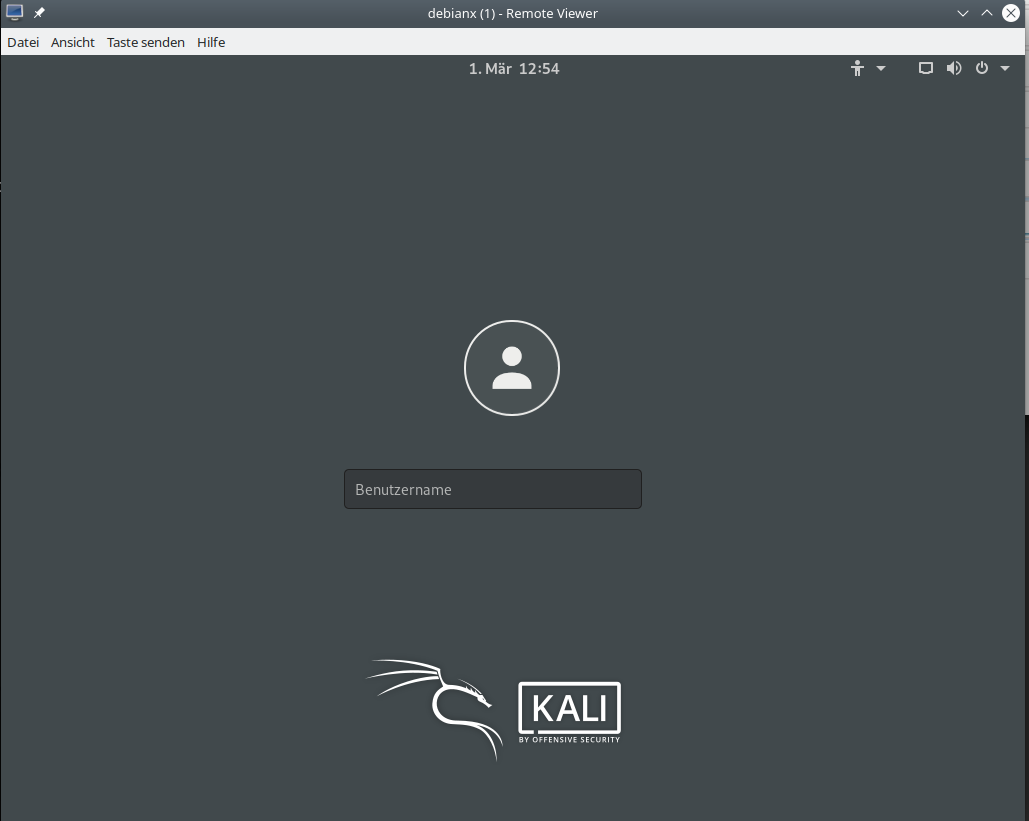
The desktop-manager may be a different one on your system. After a login to a Gnome desktop I use remote-viewer‘s menu to open a 2nd screen:
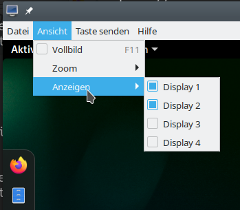
and get two resizeable screen-windows :
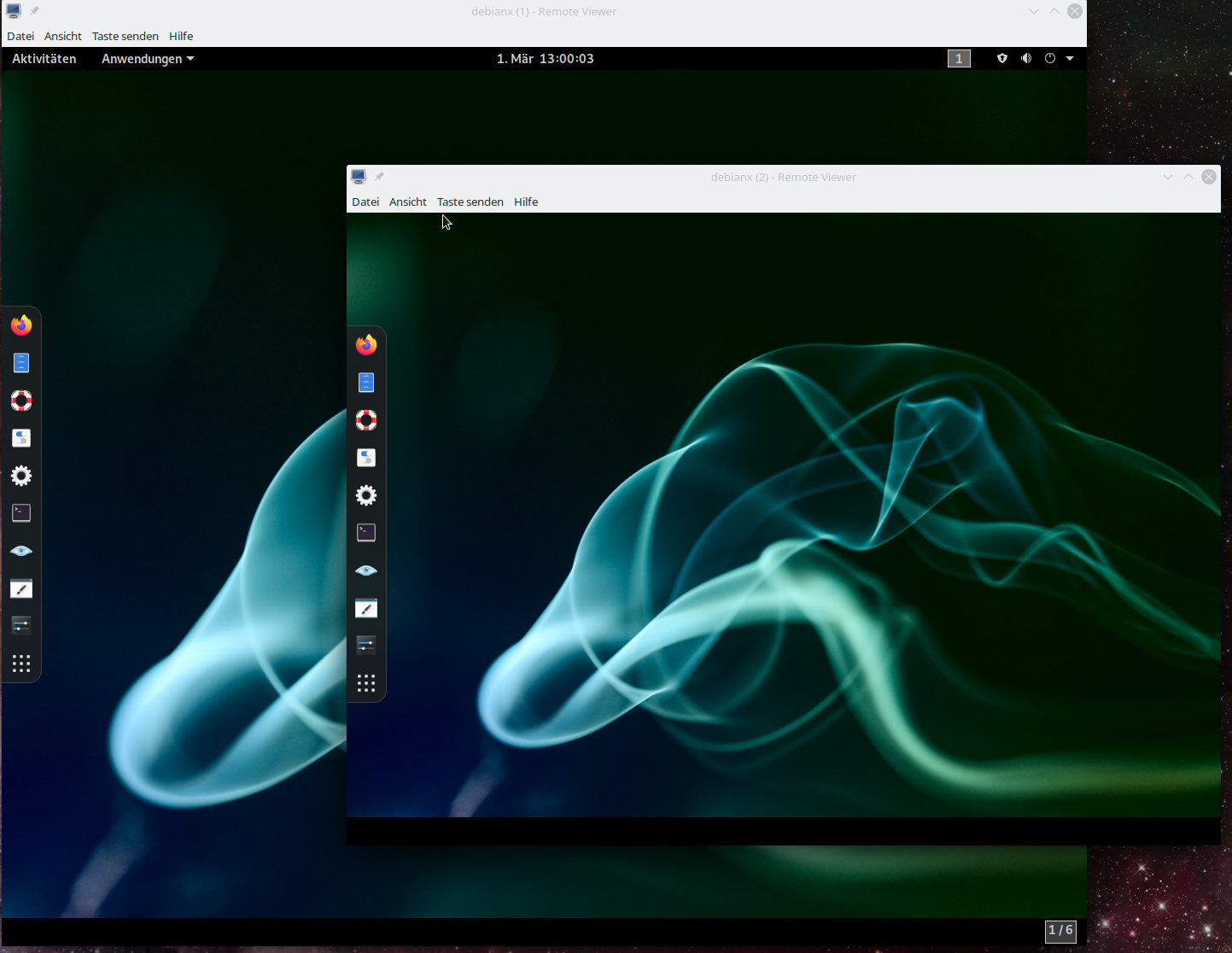
As expected! When we change the dimensions the desktop of the VM adapts to the new virtual screen sizes. Just try it out.
Will this work with a KDE desktop on the Kali guest, too? Yes, it does. KDE5 and Gnome3 can very well coexist on a Kali, Debian or Opensuse Leap15.2 (guest) system! For a Kali system you find information how to install multiple graphical desktop environments e.g. at the following links:
install-kali-linux,
kde-environment-configuring-in-kali,
kali switching-desktop-environments.
The next image shows the transparency effect of a moving terminal window on a KDE desktop of the same Kali VM – again with 2 Spice screens requested by remote-viewer:
![]()
Such effects, which can also be configured on Gnome, require an active compositor on the guest’s desktop. At least when working locally on a KVM host I never got any problems with the performance of QXL/Spice and remote-viewer with an active compositor on the guest’s Gnome, KDE, and XFCE-desktops (without OpenGL acceleration). This is a bit different on a remote system and using remote-viewer over a LAN connection; see the next articles.
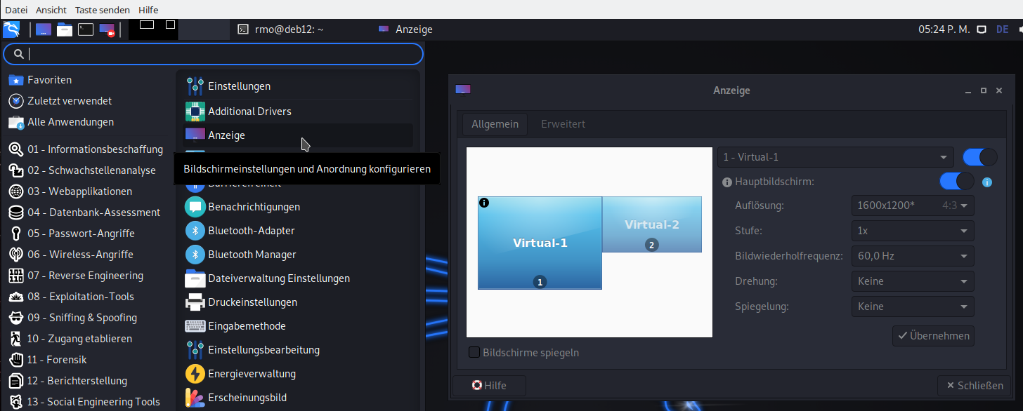
KDE and Gnome desktops on the VM automatically adapt to the sizes of the virtual screens. XFCE does not … XFCE is the present default desktop on Kali; so I installed after a distribution upgrade. Here some remote-viewer hints for XFCE fans on a VM with Kali/Debian and XFCE:
- Set the number of screens in remote-viewer to 1. After installing XFCE with ” sudo apt update && sudo apt install -y kali-desktop-xfce” and a reboot we can choose “XFCE-Session” on a button of the gdm3-screen (after having entered the username). It will the boot into a XFCE session.
- Then with the setting tool you can configure fixed resolutions for the screen displays (see below).
- Or: Just deactivate a virtual display, resize the respective window on your host’s desktop and reactivate the virtual display again in your XFCE guest. XFCE then automatically recognizes the new screen size and adapts.
- When logging out choose an option to save the desktop.

Unfortunately, XFCE has no seamless coexistence with KDE or Gome on Kali, yet. The following sequence of steps may fail:
1) Log out of a XFCE desktop-session, 2) choose a KDE or Gnome session afterwards /(this works without rebooting via the gdm menu), 3) log out of KDE/Gnome again and 4) try to restart a XFCE desktop.
On my Kali guest (on an Opensuse KVM host) I always have to reboot the guest to get a working XFCE session again, even if I did not change the screen dimensions during the KDE/Gnome session .. 🙁
Netstat reveals multiple connections corresponding to Spice channels
Using remote-viewer with a netowrk port is a really simple exercise. Most of the text above was spend on looking at the general virtualization environment. But, actually, the situation behind the scenes is not so simple. When we use netstat again, we get the following:
MySRV:/etc/libvirt/qemu # netstat -a -n | grep 20001
tcp        0      0 0.0.0.0:20001           0.0.0.0:*               LISTEN
tcp        0      0 127.0.0.1:20001         127.0.0.1:46738         ESTABLISHED
tcp        0      0 127.0.0.1:20001         127.0.0.1:46750         ESTABLISHED
tcp        0      0 127.0.0.1:46734         127.0.0.1:20001         ESTABLISHED
tcp        0      0 127.0.0.1:46750         127.0.0.1:20001         ESTABLISHED
tcp        0      0 127.0.0.1:20001         127.0.0.1:46742         ESTABLISHED
tcp        0      0 127.0.0.1:46738         127.0.0.1:20001         ESTABLISHED
tcp        0      0 127.0.0.1:46740         127.0.0.1:20001         ESTABLISHED
tcp        0      0 127.0.0.1:46748         127.0.0.1:20001
  ESTABLISHED
tcp        0      0 127.0.0.1:20001         127.0.0.1:46740         ESTABLISHED
tcp        0      0 127.0.0.1:20001         127.0.0.1:46734         ESTABLISHED
tcp        0      0 127.0.0.1:20001         127.0.0.1:46728         ESTABLISHED
tcp        0      0 127.0.0.1:20001         127.0.0.1:46744         ESTABLISHED
tcp        0      0 127.0.0.1:46728         127.0.0.1:20001         ESTABLISHED
tcp        0      0 127.0.0.1:46742         127.0.0.1:20001         ESTABLISHED
tcp        0      0 127.0.0.1:20001         127.0.0.1:46748         ESTABLISHED
tcp        0      0 127.0.0.1:46744         127.0.0.1:20001         ESTABLISHED
We find many, namely eight (8), active established connections. What do these connections correspond to? Well, they correspond to individual data exchange channels; I quote from
https://libvirt.org/formatdomain.html#video-devices:
“When SPICE has both a normal and TLS secured TCP port configured, it can be desirable to restrict what channels can be run on each port. This is achieved by adding one or more elements inside the main element and setting the mode attribute to either secure or insecure. Setting the mode attribute overrides the default value as set by the defaultMode attribute. (Note that specifying any as mode discards the entry as the channel would inherit the default mode anyways.) Valid channel names include main, display, inputs, cursor, playback, record (all since 0.8.6 ); smartcard ( since 0.8.8 ); and usbredir ( since 0.9.12 ).”
See also: spice_for_newbies.pdf
Theoretically, one should be able to use remote-viewer itself to activate or deactivate channels by setting up a “target file” for the connection; see the man-pages for more details. But on my machines it does not work neither locally not remotely. 🙁 I did not look into the details of this problem, yet ….
Testing the “one seat situation” at a Spice console
Now its time to test what I claimed in the last article: The Spice console can be accessed only by one user at a time. Let us assume, that user “uvma” is a member of the libvirt-group. Let us in addition create another user “uvmb” which is member of the group “users” on the host, only. I assume that “uvma” has opened a graphical desktop session on the KVM host (MySRV). E.g. a KDE session.
Step 1: As user “uvma” start virt-manager and boot your VM “debianx”. On a terminal window (A) use remote-viewer to open the Spice console of the VM with 2 screens. Log into a graphical desktop of the VM.
Terminal A:
uvma@MySRV:~> remote-viewer -v  spice://localhost:20001
Guest (null) has a spice display
Opening connection to display at spice://localhost:20001

(remote-viewer:20735): GSpice-WARNING **: 18:21:31.344: Warning no automount-inhibiting implementation available
Step 2: On your host-desktop open another terminal window (N) and login via “su – uvmb” as the other user. As “uvmb” now enter “remote-viewer spice://localhost:20001“.
uvma@MySRV:~> su - uvmb
Passwort:
uvmb@MySRV:~> remote-viewer -v  spice://localhost:20001
This will at once close the open two Spice windows and after a blink of a second open up one or two new Spice windows again. The effect is clearly visible.
On terminal A we get:
Guest debianx display has disconnected, shutting down
uvma@MySRV:~>
On terminal B we get a lot of warnings – but still the spice windows open in exactly the same status as we left them.
uvmb@MySRV:~> remote-viewer -v  spice://localhost:20001

(remote-viewer:20903): dbind-WARNING **: 18:25:40.853: Couldn't register with accessibility bus: Did not receive a reply. Possible causes include: the remote application did not send a reply, the message bus security policy blocked the reply, the reply timeout expired, or the network connection was broken.
Guest (null) has a spice display
Opening connection to display at spice://localhost:20001

(remote-viewer:20903): GSpice-WARNING **: 18:25:40.936: PulseAudio context failed Verbindung verweigert

(remote-viewer:20903): GSpice-WARNING **: 18:25:40.936: pa_context_connect() failed: Verbindung verweigert
Cannot connect to server socket err = Datei oder Verzeichnis nicht gefunden
Cannot connect to server request channel
jack server is not running or cannot be started
JackShmReadWritePtr::~JackShmReadWritePtr - Init not done for -1, skipping unlock
JackShmReadWritePtr::~JackShmReadWritePtr - Init not done for -1, skipping unlock
AL lib: (EE) ALCplaybackAlsa_open: Could not open playback device 'default': Keine Berechtigung

(remote-viewer:20903): GLib-GObject-WARNING **: 18:25:40.962: g_object_get_is_valid_property: object class 'GstAutoAudioSink' has no property named 'volume'
AL lib: (EE) ALCplaybackAlsa_open: Could not open playback device 'default': Keine Berechtigung

(remote-viewer:20903): GLib-GObject-WARNING **: 18:25:40.964: g_object_get_is_valid_property: object class 'GstAutoAudioSrc' has no property named 'volume'
AL lib: (EE) ALCplaybackAlsa_open: Could not open playback device 'default': Keine Berechtigung
AL lib: (EE) ALCcaptureAlsa_open: Could not open capture device 'default': Keine Berechtigung

(remote-viewer:20903): GSpice-WARNING **: 18:25:41.015: record: ignoring volume change on audiosrc

(remote-viewer:20903): GSpice-WARNING **: 18:25:41.018: record: ignoring mute change on audiosrc

(remote-viewer:20903): GSpice-WARNING **: 18:25:41.021: Warning no automount-inhibiting implementation available

(remote-viewer:20903): GSpice-WARNING **: 18:25:41.052: playback: ignoring volume change on audiosink

(remote-viewer:20903): GSpice-WARNING **: 18:25:41.052: playback: ignoring mute change on audiosink
The warnings are mainly due to the fact that user “uvmb” has no rights to access the Pulseaudio context of the desktop of user “uvma”. (I take care of Pulseaudio in one of the next articles …) At the first switch between the users you may only get one Spice window as “uvmb”. Choose two screens then. Afterwards you can switch multiple times between the users uvma and uvmb. Two windows get closed for the user with present Spice console session, two windows are opened for the requesting user, and so on.
Conclusion: “uvmb” and “uvma” can steal each other the Spice console with remote-viewer as and when they like.
By the way: A Spice console can be left regularly by a user by just closing the Spice client window(s). Note that this will not change the status of your desktop session on the host! This is left open – with all consequences.
Restricting access by setting a password
Let us prevent being thrown of the “seat” in front of our Spice console. As root change the <graphics> definition in VM’s definition file to
...
 <graphics type='spice' port='20001' autoport='no' listen='0.0.0.0' keymap='de' passwd='spicemeandonlyme' defaultMode='insecure'>
      <listen type='address' address='0.0.0.0'/>
      <image compression='off'/>
      <gl enable='no'/>
    </graphics>
   ...
If you haven’t noticed: The relevant difference is the “passwd” attribute. You could have added this setting via virt-manager, too. Try it out.
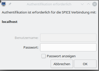
Shut down and restart your VM. Any user that now wants to access the Spice console using “remote-viewer spice://
localhost:20001” will be asked for a password. You yourself, too, if you close the console and try to reopen it.
Regarding security: The password transfer will to my understanding be AES encrypted. See Daniel P. Berrangé’s blog https://www.berrange.com/posts/2016/04/01/improving-qemu-security-part-3-securely-passing-in-credentials/. But as long as the rest of the data exchange with the VM is not encrypted, this precaution measure won’t help too much against ambitioned attackers.
Conclusion
Using remote-viewer locally on a KVM host in combination with a network port to access a VM’s graphical Spice console is easy and convenient. It requires a minimum of settings. In addition it offers up to four virtual screens which you can open via a menu.
However, using a network port implies security risks. You should think about proper counter-measures first if you want to lean on “remote-viewer”. Once configured in the way described above there is no libvirt-layer or anything else which may hinder ambitious attackers to analyze the unencrypted data flow between the Spice client and the VM through the host’s network port.
In the next article
I want to show you how one can configure the VM such that remote-viewer can access the Spice console via a local Unix port. A network port is not opened in this approach. Security is none the less hampered a bit as we have to give a standard user some rights which normally only the “qemu” group has. But we shall take care of this aspect by using ACLs.
Links
Virtualization on Opensuse
https://doc.opensuse.org/ documentation/ leap/ virtualization/ single-html/ book.virt/index.html
Libvirtd daemon
https://www.systutorials.com/docs/linux/man/8-libvirtd/
Libvirt connection URIs
https://libvirt.org/uri.html
Find the Spice URI to use
https://access.redhat.com/ documentation/ en-us/ red_hat_enterprise_linux/7/ html/ virtualization_deployment_and_ administration_guide/ sect-Domain_Commands- Displaying_a_URI_ for_connection_to_a_graphical_display
General Kali installation
https://www.cyberpratibha.com/blog/how-to-update-and-upgrade-kali-linux-to-latest-version/
KDE, XFCE on Kali
https://technicalnavigator.in/kde-vs-xfce-which-one-is-better/