KMeans as a classifier for the WIFI and MNIST datasets – I – Cluster analysis of the WIFI example

In the November and December 2021 editions of the German “Linux Magazin” R. Pleger discussed a simple but nevertheless interesting example for the application of a cluster algorithm. His test case was based on a dataset of the UCI Irvine. This dataset contains 2000 samples with (fictitious?) data describing WIFI signals which stemmed from seven WLAN spots around a building. The signal strength of each source was measured at varying positions in four different rooms. I call the whole setup the “WIFI example” below.

One objective of the articles in the Linux Magazin was to demonstrate how simple it is today to apply basic Machine Learning methods. In a first step the author used a ML classifier algorithm to determine the location (i.e. the room) of a measuring instrument just from the strengths of the different WIFI signals. This task can be solved by a variety of algorithms – e.g. by a Decision Tree, SVM/SVC or a simple Multilayer Perceptron. The author used Sklearn’s RandomForestTree. This method is a good example for the powerful “Ensemble Learning” technique. When applied to the simple and well structured WIFI example it predicts the rooms for test samples with an accuracy of more than 98%.

The author afterward performed a deeper analysis of the WIFI data via Kmeans, MiniBatchKMeans and PCA. His second article underlined a major question, which sometimes is not taken seriously enough:

Do the data, which we feed into ML algorithms, really cover all aspects of the problem? Is the set of target labels complete or sufficient in the sense that the separation of the samples into labeled groups really reflects the problem’s internal structure? Or do the data contain more information than the labels reveal?

Unfortunately, in my opinion, the Linux Magazine covered an important point, namely the relation of the results of a PCA analysis to a 2-dimensional cluster visualization, in an incomplete and also slightly misleading way. In addition another interesting question was not discussed at all:

Can we use KMeans also as a classifier? How would we do this?

In this series of posts I want to dig a bit deeper into these topics – both for the WIFI example and also for the MNIST dataset. For MNIST we will not be able to visualize clusters as easily as for the WIFI example. Therefore, we should have a clear idea about what we do when we use clusters for classifying.

In this first post I focus on the results of a cluster analysis for the WIFI example. In a second article I will discuss the relation of cluster results to a PCA analysis. A third post will then present a very simple method of how to turn a cluster algorithm into a classifier algorithm. In later articles we shall transfer our knowledge to the MNIST data. More precisely: We shall combine a PCA analysis with a cluster classifier to predict the labels of handwritten digit images. We will use the PCA technique to reduce the dimensions of the MNIST feature space from 784 down to below 80. It will be interesting to see what accuracy we can reach with a relatively crude clustering approach on only about 30 main PCA components. As a side aspect we shall also have a look at standardization and normalization of the MNIST data.

I do not present any code in the first three posts as the required Python programs can be build relatively straight-forward and most of the core statements were already given in the Linux Magazin. You unfortunately have to buy the articles of the magazine; but see https://www.linux-magazin.de/ausgaben/2021/11/maschinenlernen/. However, as soon as we turn to MNIST I shall provide a Jupyter notebook.

The WIFI example: Two thousand samples, each with data for the signal strength of seven WLAN sources measured in four rooms

You can download the data WIFI data set from the following address:
https://archive.ics.uci.edu/ml/machine-learning-databases/00422/wifi_localization.txt

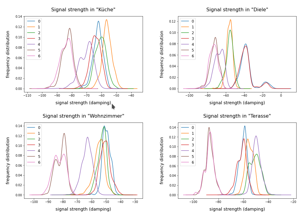
The feature space of this is example is 7-dimensional: 7 WLAN spots provide WIFI signals in the building. We have 2000 samples. Each sample provides the signal strength of each of the WLAN sources measured at different times and positions within a specific room. An integer number in [1,4] is provided as a label which identifies the room. The following plot shows the interpolated frequency distribution over the signal strength for each of the 7 signals in the four rooms:

Cluster analysis of the WIFI data – more than four rooms?

The original label-data of the WIFI example imply the existence of four rooms. But can we trust this information? The measurements in the room, which we called “Diele” in the plots above, indicate a consistent second peak for both the signals 0 and 3. Is this due to an opening into another room?

A simple method to analyze the inner structure of the distribution of data points in a configuration or feature space is a “cluster analysis”. The KMeans algorithm provides such an analysis for an assumed number of clusters.

KMeans is a basic but important ML method which reveals a lot about the data distribution in feature space and indirectly about the complexity of hyperplanes required to separate data according to their labels. Among other things KMeans determines the positions of cluster centers – the so called centroids – by measuring and systematically optimizing distances of samples to assumed centroids. Actually, the sum over all intra-cluster variances, i.e. the summed quadratic distances of the associated samples to their cluster’s centroid, is minimized. The respective quantity is called “inertia” of the cluster distribution. See e.g. the excellent book of P. Wilmott, Machine learning – an applied mathematics introduction” on this topic.

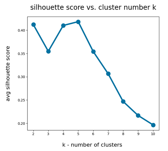
A simple method to find out into how many clusters a distribution probably segregates is to look for an elbow in the variation of the inertia with the number of clusters. When we look at the variation of inertia values with the number of potential clusters “k” for the WIFI example we get the following curve:

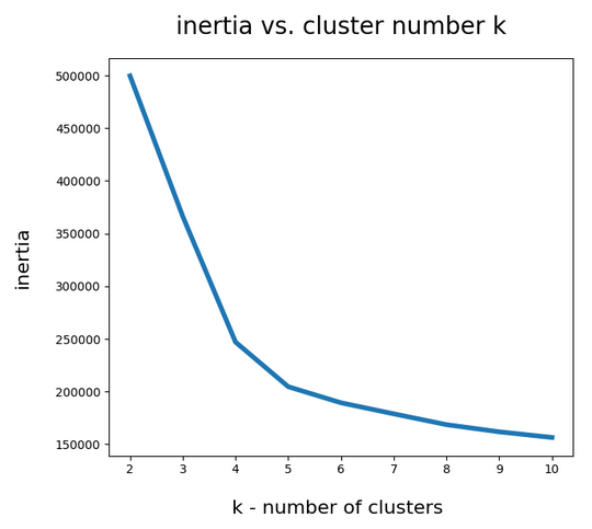
This indicates an elbow at k=4,5.

Another method to identify the most probable number of distinct clusters in a multi dimensional data point distribution is the so called “silhouette analysis”. See the book of A. Geron “Hands-On Machine Learning with Scikit-Learn, Keras and Tensorflow”, 2n edition, for a description. For the WIFI example the plots of the silhouette score data support the result of the elbow analysis:

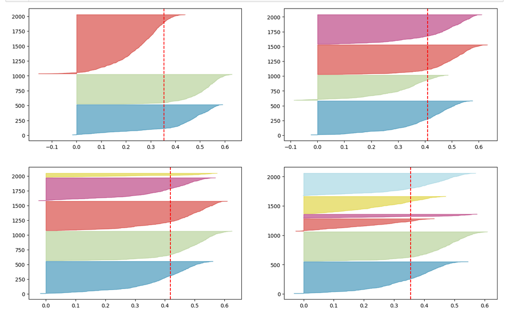
The second plot shows ordered silhouette data for k = 3,4,5,6 clusters. Again, we get the most consistent pictures for k=4 and k=5.

So, the data indicate a fragmentation into 4 or 5 clusters. How can we visualize this with respect to the feature space?

Scatter plots for 2-dim sub-spaces of the feature space

A general problem with the visualization of cluster data for multidimensional data is that we are limited to 2, maximal 3 dimensions. And a projection down to two dimensions may not reflect the real cluster separation in the multidimensional feature space in a realistic way. But sometimes we are lucky.

We shall later see that there are two primary components which dominate the data and signal distributions in the WIFI example. A major question, however, is whether we will also find that only a few original features contribute dominantly to these major components. A PCA analysis does not mean that a “primary component” only depends on the same number of features!

As I did not know the relation of “primary components” to features I just plotted the results of “KMeans” for a variety of 2-dim signal combinations. I used Sklearn’s version of KMeans; due to the very small data ensemble KMeans is applicable without consuming too much CPU time (this will change with MNIST; there we need to invoke MiniBatchKMeans):

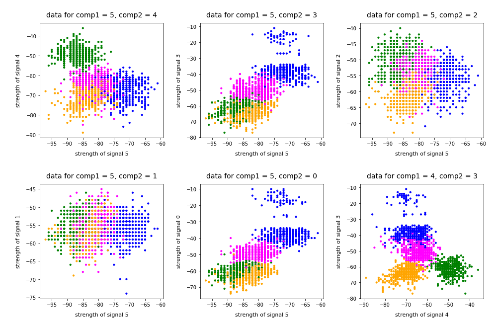
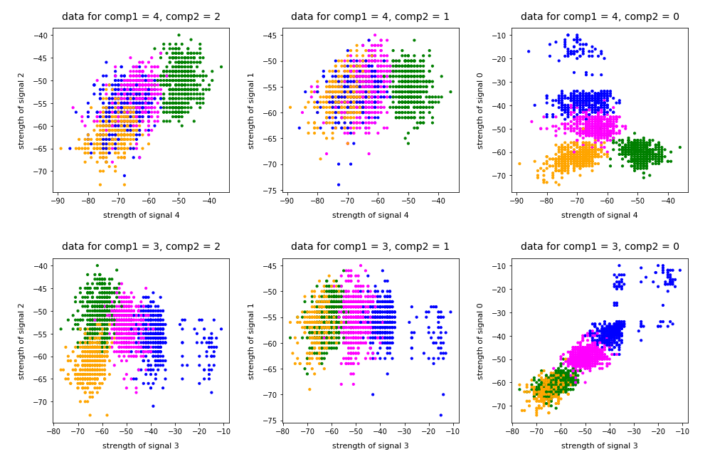
Note that the colorization of the data points in all plots was done with respect to the cluster number predicted by KMeans for the samples – and not with respect to their labels.

It is interesting that the projections onto two special feature combinations – namely WLAN-4/WLAN 0 and WLAN-3/WLAN-0 signal – show a very distinct separation of the clusters.

Four or five clusters ?

The data displayed above depend a bit on the initial distribution of cluster centers as an input into the KMeans algorithm. But for 4 and 5 clusters we get very consistent results. The next plots show the positions of the centroids:

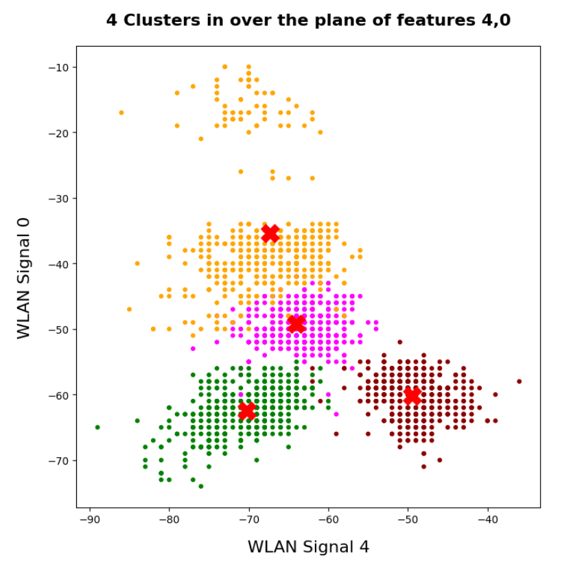
This time the colorization was done with respect to the labels. What we see is: Five clusters represent the situation a bit better than only 4 clusters.

When we align this with the rooms: Five “rooms” may describe the signal variation better than only 4 rooms. The reason for this might be that one of the four rooms has a wall which partially separates different areas from another. We often find this in “entrances” [German: “Diele”] to houses. Sketches of the rooms in the Linux Magazin article actually show that this is the case. And, of course, such a wall or an opening into another room would have an impact on the damping of the WLAN signals.

Addendum 19.03.2022: Comparing clusters with groups of labeled data points

An important question which we have not answered yet by the images shown above is the following:

How well do clusters coincide with groups of data points having a specific label?

Note that in general you can not be sure that clusters reflect data points of the same label. Actually, a cluster is only a way to describe a close spatial vicinity of data points in some region of the multidimensional feature space. I.e. some kind of clumping of the data points around some centroids. But spatial vicinity does not necessarily reflect a label: A label border may often separate data points which are very close neighbors. And a cluster may contain a mixture of samples with different labels ….

Well, in the case of the WIFI example the identified 4 to 5 clusters match the groups of data points with different labels quite well. Below I superimposed the sample’s data points with different colors: First I colorized the data points according to their label. On top of the resulting scatter plot I placed the same data points again, but this time with a different and transparent colorization according to their cluster association. In addition I shifted the second data layer a bit to get a better contrast:

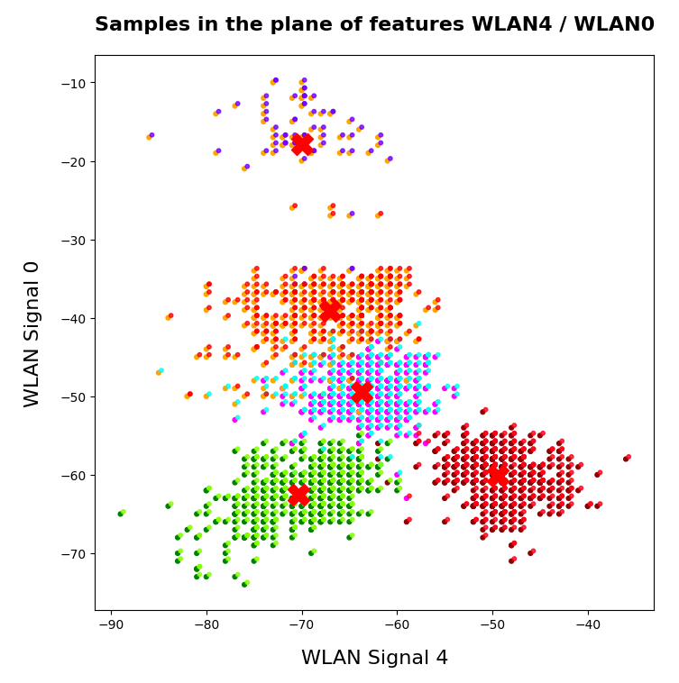
You see that the areas are not completely identical, but they overlap quite well. Obviously, I used 5 clusters. Also the fifth cluster fits well into a region characterized by just one label.

Conclusion

The simple WIFI example shows that a cluster analysis may give you new insights into the structure of ML data sets which a simple classifier algorithm can not provide. In the next article

KMeans as a classifier for the WIFI and MNIST datasets – II – PCA in combination with KMeans for the WIFI-example

we shall link the information contained in the “clusters” to the results of a PCA analysis of the WIFI example.

Stay tuned …

Ceterum censeo: The most important living fascist which must be denazified is the Putler.

Blender – complexity inside spherical and concave cylindrical mirrors – IV – reflective images of a Blender variant of Mr Kapoor’s S-curve

The topic of the last post in this series

Blender – complexity inside spherical and concave cylindrical mirrors – I – some impressions
Blender – complexity inside spherical and concave cylindrical mirrors – II – a step towards the S-curve
Blender – complexity inside spherical and concave cylindrical mirrors – III – a second step towards the S-curve

was the construction of a metallic object with basic similarities to the “S-curve” of artist Anish Kapoor. Our object was a bit more extreme than the artists real object; we had a smaller curvature radii in two dimensions and on the outer ends our surface approximated a half circle boundary curve. We therefore could expect multiple reflections of light rays on the concave side(s) of our virtual object when applying ray tracing.

At the end of my last article I already presented some images of the reflection of a far distant horizontal line marked by a sun close to the horizon at dusk or dawn. In this article I am going to add some simple objects – a small red and a small green sphere at varying positions. Plus a point like light source. I take some shots with the virtual Blender camera form different angles and with varying focal length. I present the results below without many comments.

What we see is a rich variation of patterns and figures. Mathematically it is all the result from a single and simple mapping-operation. Each operation maps one point on our surface to another point on the S-curve (or on a hit sphere). The points are given by millions and millions of light rays which in the end reach our virtual camera from different angles. The basic message is:

Simplicity can create a complexity which or brain would not predict without some deeper analysis. And a complex apparition may be based on simple rules and the selection of special circumstances.

So, besides many other philosophical aspects Mr. Kapoor’s “S-curve” reveals a very fundamental idea in physics, certain branches of mathematics and in information theory.

Reflections of a horizon line

Reflections of a horizon line and a red sphere

Reflections of a horizon line, a red and a green sphere

Note that the concave side of the S-curve gives us a first idea about what we can expect from a full half-sphere where even more reflections on the surface are possible before a light ray reaches the camera.

But, in my next article
Blender – complexity inside spherical and concave cylindrical mirrors – V – a video of S-curve reflections
I am first going to produce a movie of objects moving in front of the concave part of the S-curve.


Blender – complexity inside spherical and concave cylindrical mirrors – III – a second step towards the S-curve

I continue with my mini-series on how to (re-) build something like the S-curve of Mr. Kapoor in Blender. See :

Blender – complexity inside spherical and concave cylindrical mirrors – I – some impressions

In my last post

Blender – complexity inside spherical and concave cylindrical mirrors – II – a step towards the S-curve

I discussed how we can add a smooth transition from convex and concave curvature around the y-axis of an originally flat rectangular Blender mesh positioned in the (y,z)-plane. The rectangle had its longer side in y-direction. Starting from a flat area around the vertical middle axis (in z-direction) of the object we bent the wings to the left and right around the y-axis with systematically growing curvature, i.e. with shrinking curvature radius, in y-direction. The curvature around the y-axis left of the central z-axis got a different sign than the curvature right of the central z-axis. At the outer edges of both wings we approximated the form of a half cylinder. So curvature became a function of both x and y.

To create a really smooth surface with differentiable gradient and curvature we had to apply a modifier called “Subdivide Surface“. The trick to make this modifier work sufficiently well with only a few data points in z-direction was to keep curvature almost constant in z-direction for a given y-position along the horizontal axis. We achieved this by putting the vertices of our mesh on the central rotation-axis at the same z-(height)-values as the vertices on the circles at the outer edges. In the end we had established a smoothly varying gradient of the surface curvature around the y-axis with the y-coordinate while the partial derivative in z-direction of this curvature was close to zero for any fixed y-position.

In this post I want to add an “S-curvature” of the object in y-direction. Meaning: We are now going to bend the object along a S-shaped path in the (x,y)-plane. Physically, we are adding curvature in x-direction, more or less constant around two imaginary vertical axes positioned at some distance in y-direction from the central z-axis – and with different signs of the curvature. So, we are creating a superposition of a growing curvature around the y-axis with a constant curvature around two z-axes for each of the wings left and right of the central rotational z-axis of our object. Eventually, we build something like shown below:

When we look at images of Mr. Kapoor’s real S-curve we see that he keeps curvature at zero both in z- and a diagonal x/y-direction at the central rotational axis – due to the “S”. The same is true for our object. But: In comparison to the real S-curve of Mr. Kapoor our object is more extreme:

The ratio of height in z-direction to length in y-direction is bigger in our case. The object is shorter in y-direction and thus relatively higher in z-direction. The curvature radii around the y-axis are significantly smaller. Our surface approximates full half circle curves at the outer edges; in contrast to the real S-curve our surface approximates a shifted cut of a cylinder.

We could, of course, adapt our S-curve in Blender a bit more to the real S-curve. However: Our more extreme bending around the y-axis at the outer left and right edges of the object allows for multiple reflections of light falling in in x-direction on the concave sides of the object. This is not the case for the real S-curve.

Steps to give the surface an S-shape

How do we get to the surfaces presented in the above figures in Blender? The following steps comprise building a suitable symmetric and very fine grained Bezier-path and the use of a curve modifier. To achieve a relatively smooth bending in x-direction we must first subdivide our original object in sufficient sections in y-direction in addition to the already existing subdivisions in z-direction.

Step 1: Sub-dividing our object in y-direction

The final object mesh constructed in my last post is depicted below:

We “apply” (via menu “Object” > “apply”) any rotations we may have done so far. The object’s center should now coincide with the world center. We position the camera some distance apart in x-direction from our object, but at y=z=0. The following image shows the camera perspective.

Remember that our object consists of two meshes which we have joined at the central axis. We are now going to separate each half in 32 sections in y-direction.

Go to Edit mode, position the cursor in one half and press Ctrl-R:

Turn your mouse wheel until you have created 32 subdivisions. (The number is shown at the bottom left of your view-port). Left click twice to fix the subdivision lines at their present positions; do NOT move the mouse in between the clicks.

Doing this on both halves eventually gives us:

We check that y- and x-distances of the vertices have equal absolute values. We in addition check z-heights for selected vertices and compare them to the height of vertices on the outer circles.

Step 2: Design a S-path

We move our object, which has dimensions of 6m in y-direction and 2m in z- and x-direction, respectively, to the left (y=-6m). Just to get some space at the world origin. We now add a Bezier curve to our scene. Its origin is located at the world center and it is stretched along the x-axis. Rotate the curve around the z-axis by 90 degree such that it stretches along the y-axis. Choose a top-view position and rotate the viewport such that the y-axis points to the right.

Stretch the curve to an y-dimension of 6m. Select the curve. Go to edit mode. We now rotate the rightmost and the leftmost tangent bars such that we get the following curve:

You fix the required symmetry by watching and adjusting the position information of the tangent bar\’s end vertices in the sidebar of the viewport. Note that a tangent bar has 2 associated handles and vertices. By changing vertex positions systematically to [(x=-0.5, y= -3.5), (x=0.5, y= -2.5)] and [(x=-0.5, y=2.5), (x=0.5, y=3.5)] on the left and the right side, respectively, you get a seemingly nice flat S-Curve.

Go to object mode and change the dimension of the curve in x-direction to 2m. You then clearly see that the path is not a very smooth one, but consists of distinguished linear segments. This would be a major problem later on. In addition the curvature for the S seems to be a bit extreme. We change the x-dimension to just 1 m. Then we subdivide the curve into further segments in Edit mode. Multiple times.

And we get a smoothly curved and well dimensioned path:

Eventually, we end up with the following situation:

Step 3: Apply a curve modifier to our object

Now comes an important point: If you have assigned the origin of the curve to its midpoint, you should do the same with your object- see the Internet for appropriate Blender operations:

We then move our object to y=3.171m and z=1m, i.e. a bit further than rightmost end-point of the path and above the worlds central plane.

Now, we add a curve-modifier to our object, select the Bezier curve (our path) and get

We center our view and choose a top-position. We adjust the y-location of the object until its present center coincides with the world center

And there we have our personal S-curve – more extreme than Kapoor’s real S-cure – but this is only a question of dimension adjustments AND the right choice of how to cut the limiting circle mesh in the beginning (see the last post). Our S-curve will show multiple reflections on its concave side(s).

Apply the modifier “subdivision surface”

The rest is routine for us already. We apply the subdivision surface modifier to get a smooth surface.

When we modify the world’s sky texture a bit with a sun just at the horizon then we get images like the following just from the horizon line and from different camera perspectives with different focal lengths (wide angle shot).

We clearly see multiple reflections in vertical direction on the left concave side of our object.

Complexity out of simple things … Real fun …

Conclusion

Rebuilding something like the S-curve of Mr. Kapoor was hard work for me who uses Blender just as a hobby tool. But it was worth the effort. In my next post,

Blender – complexity inside spherical and concave cylindrical mirrors – IV – reflective images of a Blender variant of Mr Kapoor’s S-curve

I am going to show what happens when we place objects in front of our S-curve. This will give us a first impression of what might happen with a totally concave surface as an open half sphere.
Stay tuned …


Blender – complexity inside spherical and concave cylindrical mirrors – II – a step towards the S-curve

In my last post

Blender – complexity inside spherical and concave cylindrical mirrors – I – some impressions

I briefly discussed some interesting sculptures and optical experiments in reality. The basic ideas are worth some optical experiments in the virtual ray-tracing world of Blender. In this post I start with my trial to reconstruct something like the so called “S-curve” of the artist Anish Kapoor with Blender meshes.

If you looked at the link I gave in my last article or googled for other pictures of the S-curve you certainly saw that the metallic surface the artist placed at the Kistefoss museum is not just a simple combination of mirrored cylindrical surfaces. It is much more elegant:

The first point is that it consists of one continuous coherent piece of metal. The surface is deformed and changes its curvature continuously. It shows symmetry and rotational axes. When my wife and I first saw it we stood at a rather orthogonal position opposite of it. We only got aware of the different cylindrical deformations on the left and right side. We wondered what Kapoor had done at the middle vertical axis as we expected a gap there. Later we went to another position – and there was no gap at all, but a smooth variation of curvatures along the main axes of the object.

The second point is the combination of different curvatures: a cylindrical curvature in vertical direction (mirrored in left/right direction) plus the elegant S-like curvature in horizontal direction. The curvature in vertical direction grows with horizontal distance from the center – it is zero at the central vertical axis. The left and right part of the object are identical – they reflect a 180 °ree; rotation (not a mirroring process) around the central vertical axis. Actually, the gradient at the central rotational axis and the along the horizontal symmetry axes disappears. And no curvature at all at the central vertical axis.

All in all a lot of different symmetries and smooth curvature transitions! The artist plays with the appeal of symmetries to the human brain. But, at the same time, he breaks symmetry strongly in the visual impression of the viewer with the help of the rules of optics. Wonderful!

In this article I want to tackle the problem of a smooth transition between two cylindrically deformed surfaces in Blender first. The S-curvature is the topic of the next post.

The result first

I first show you what we want to achieve:

We get an impression of the mirroring effects in “viewport shading mode” by adding a sky texture to the world background and a simple textured plane:

The reader may have detected small dips (indentations) at the centers of the upper and lower edge. I come to this point later on. Compared to the real S-curve a major difference in vertical direction is that Kapoor did not use a the full curvature of a half cylinder at the outmost left and right ends. He maybe took only a cut off part of a half circle there. But what part of a half-circle you use in the end is a minor point regarding the general construction of such a surface in Blender.

How to get there?

As I only use Blender seldom I
really wondered how to create a surface like the one shown above. Mesh based or nurbs based? And how to get a really smooth surface? Regarding the latter point you may think of subdivisions, but this is a wrong approach as a subdivision of a mesh intersects linear connections between vertices. Therefore, if you applied simple subdivision to the object you would create points not residing on a circle/cylinder/surface – which in the end would disturb the optics by visible lines and flat planes. Even if you added a smoothing modifier afterward.

The solution in the end was simple and mesh based. There is one important point to note which has to do with rules for object creation in Blender:

You define the resolution of the mesh(es) we are going to construct in the beginning!

As we need to edit some vertex positions manually the resolution in first experiments should rather be limited. For a continuous surface we shall apply a surface smoothing modifier anyway. This modifier rounds up edges a bit – which leads to the “dips” I mentioned. They will be smaller the higher you choose the meshes’ resolution – but this is something for a final polished version.

Constructional steps

All in all there are many steps to follow. I only give a basic outline. Read the Blender manual for details.
Note: I added the application of a modifier in the middle of the steps for illustration purposes. You should skip this step and apply the modifier only in the end. I sometimes experienced strange effects when applying and deleting the modifier during work with vertices.

Step 1: You first create a mesh based circle. You now decide which number of mesh nodes and basic resolution of the later surface you want to have. This is done by the the tool menu that opens in Blender version 2.82 in the lower left of the viewport. Lets keep to the standard value of 32 mesh points (vertices). This obviously means that a half-circle later on will contain 17 vertices. All vertices of our first reside exactly on the circle line. The circles center resides at the global world center. You also see that 4 points of the circle sit on the world axes X, Y. Leave the circle exactly where it is. Do not apply any translation. (It would be hard to realign it with world axes later on.)

Step 2: Change to Edit mode and remove one side of the circle (left of the X-axis) by eliminating the superfluous vertices. Do it such that the end points of the remaining half-circle reside exactly on the X-axis of the world mesh. Keep the origin of the mesh were it is. Do NOT close the circle mesh on the X-axis, i.e. do not create a closed loop of vertices!

Step 3: You then add a line mesh in Object mode. This can e.g. achieved by first creating a path. Move it along the world Y-axis to get some X-distance from the half-circle (-3m). Select the path by right clicking and convert the path to a mesh by the help of a menu point. Go to Edit mode again and eliminate vertices (or adding by subdividing) – until the resulting line mesh has exactly the same number of vertices (17) as your half circle (including the end points). In object mode set the origin to the mesh’s geometry, i.e. its center. Move the line mesh to X=0. Change its X-dimension to the same value the half circle has (2m).

Step 4: Rotate the half-circle by 90 degrees around the X-axis to get a basic scene like in the picture below. Join the two meshes to one object.

Step 5: Go to Edit mode and provide missing edges to connect the line segment with the half-circle.

Step 6: Add faces by selecting all vertices and choosing menu point “Face > Grid Fill”.

Hey, this was a major step. save your results – and make a backup copy for later experiments.

Step 7: Add a Sky Texture to the world. Activate the Cycles renderer. Rotate the object by 90 degree around the Y-axis. Choose viewport shading mode.

Step 8: Move object to Z=1m. Right click in Object mode on your object it; choose “Shade smooth”.

Just to find that you still see the edges of the faces. Smooth is not really smooth, unfortunately.

Step 9: Skip this step in your own experiment and perform it at the end of our construction. Just for illustrating that the flat surfaces can be eliminated later on, I add a modifier to our object – namely the modifier “subdivision surface” – which offers a more intelligent algorithm than “Shade smooth”. Just for testing I give it the following parameters:

We get:

Much more convincing! You see e.g. at the left side that the corners have been rounded – this will later lead to the dips I mentioned.

Intermediate consideration
We could now duplicate our object, rotate the duplicate and join it with the original. But before we do this we change the height values of the vertices along the left edge (actually a line segment). From our construction it is clear that corresponding vertices on the half circle and the left edge cannot have the same Z-coordinate values – they reside at different heights above the ground. The “catmull clark” algorithm of our modifier therefore creates a surface with gradients and curvature varying in all coordinate directions. There is no real problem with this. However, we reduce the chance for certain caustics and cascades of multiple reflections on the concave side of the final surface. Cylindrical surfaces (i.e. with constant curvature) give rise to sharp reflective caustics. To retain a bit of this and keep the curvature rather constant in Z-direction (whilst varying in X-direction), we are going to adjust the heights of the vertices along the straight left edge to the heights of the vertices along the half-circle.

Step 10: Go to edit mode. Do NOT move the vertices of the half circle! Check the Z-value of each of the vertices of the half-circle by selecting one by one and looking at the information on
the sidebar of the Blender interface (View > Sidebar). Change the Z-coordinate of the half-circle’s counterpart on the left straight edge to the very same value. Repeat this process for all vertices of the half-circle and the corresponding ones of the straight edge.

You see that the vertices are now non-equidistantly distributed along the Z-axis on the left side !
This gives us already a slightly different shading in the lower part.

Step 11: Important! Remove the modifier if you applied it. Then: Move the object such that all vertices on the left corner are at Y=0 and X=0. For Y=0 you can just adjust the median of the vertices. Check also that the corners of the half-circle have X=0 and Y=3. All vertices of the half circle should have Y=3.

Then snap the cursor to the grid at X=0, Y=0, Z=1. Afterward snap the origin of the object to the cursor. The object’s coordinates should now be X=0, Y=0, Z=1.

Step 10: In Object mode: Duplicate the object by SHIFT D + Enter. Do not move the mouse in between; don’t touch it. Rotate the active duplicate around the Z-axis by 180 degrees.

Check the coordinates of the vertices of the mirrored object. If its right vertices reside at y=0 and its left at y=-3 then join the two objects to one. Note: At the middle there are still two rows of vertices. But their vertices should coincide exactly at their x=0, Y=0 and Z-values. If not you will see it later by some distortions in the optics.

Step 11: Add a metallic material

Place the camera at

and add
the modifier again with the settings given above. Render with the help of the material preview:

Step 11: Add a Sun at almost 180 degrees and play a bit with the sky

We get in full viewport shading:

Watch the sharp edges created by multi-reflections on the left concave side of the object. This we got due to our laborious adjustment of the Z-coordinates of our central vertices.

Save your result for later purposes!

Adding some elements to the scene

After having created such an object we can move and rotate it as we like. In the following images I mirrored it (2 rotations!). The concave curvature is now at the right side. Then I added a plane with some minimum texture with disturbances. Eventually, I added some objects and extended light sources, plus a change of the sun’s color to the red side of the spectrum. (Hint: When moving around spacious light sources relatively close to the object the reflections should not show any straight line disturbances. Its a way to test the smoothness of your surface created by the modifier.)

Yeah, one piece of metal with growing cylindrical concave and convex curvatures to the left and the right. We are getting closer to a reconstruction of the S-curve. And have a look at the nice deformations of the reflected images of a red cylinder, a green cone and a blue sphere, which I have placed relatively closely to the concave surface on the right side. Physics and Blender are fun! But all respect and tribute again to Anish Kapoor for his original idea!

In the next post

Blender – complexity inside spherical and concave cylindrical mirrors – III – a second step towards the S-curve

I have a look at an additional S-curvature in horizontal direction. Stay tuned ..


Blender – complexity inside spherical and concave cylindrical mirrors – I – some impressions

After two stressful months at my job I used part of my Christmas holidays to play a bit around with Blender. For me Blender has always been a fascinating tool to perform optical experiments with mirrors, lenses, light emitting gases, etc. It’s real fun … like in a virtual lab. See e.g. the image of two half-transparent cubes intersecting each other in an asymmetric way; the cubes were filled with volumetric gas emitting red and green light:

The idea for the experiment illustrated above arose in a discussion with a German artist (Michael Grossmann) about different kinds of color mixtures. The human eye and the neural networks behind it interpret a dense mixture of green and red light rays as yellow. This is true only for active light emitters, but not for passive reflective particles as used in painting. Think of pixels emitting light on a TV-screen: There neighboring red and green pixels create an impression of yellow.

In this present article series, however, I want to describe two experiments for highly reflective mirroring surfaces. I got the ideas from two real art installations. All credit must be given to the artists behind the original art objects:

One object is located in a sculpture park in Norway called “Kistefoss museum”. See https://www.kistefosmuseum.com/ sculpture/ the-sculpture-park. I warn you – a visit to this park is really expensive in my opinion (18 Euros per person + 8 Euros or more for parking. OK, the fact that enjoying modern art is a kind of luxury had to be expected in the richest country outside the EU. And, of course, Kistefoss is run by a private investor …. See https://www.kistefos.no/. Some things obviously never change during the history of capitalism. Presently the impression of art in original “nature” of an originally beautiful river valley is spoiled by a huge construction site for a 4 or 6 track autobahn bridge. Well, well – so much about the relation between art and capitalism.

Nevertheless – there are some really nice installations at Kistefoss to look at.

The object I refer to is named “S-Curve” and was made by the well known contemporary artist Anish Kapoor. See “https://www.kistefosmuseum.com/ sculptur/ s-curve” or google for “s-curve anish kapoor” and look at the images. The installation consists of a bent elongated rectangular metallic surface looking like a twisted curved band. Curved in two directions: The curvature on the left side of the s-curved band is concave, on the right side it is convex. I found this idea of combining reflective concave and convex mirror surfaces breathtakingly simple and impressive at the same time. The whole installation makes you think about the reality behind visual images triggered by some conceptional network in your brain. It reminded me of the old Platonic idea that our relation to the real world must be compared to a man sitting in a cave where he only sees shadows of a real world on a wall. Now, imagine a world where our cave walls where made of curved mirrors – how could we get a clue about the reality behind the strange reflections? Well, such questions seemingly trigger something inside physicists …

The second public installation is located in the Norwegian city of Drammen at a river bank. There you are confronted with highly reflective outer surfaces of two spheres on each side of the river. However, these spheres also have a kind of spherical indentation on their outer sides. Sometimes when the
sun is at the right position you can see strange ring like reflections of light in these indentations – with rater sharp edges. Similar disturbing effects can be seen when you put some intensive LED lamp outside and inside the sphere. Makes you wonder what kind of images an open half-sphere would create.

The question what a camera placed at different positions in front or inside a reflective open half-sphere is for many reasons interesting if you start thinking about it with some recovered school knowledge about optics. Three major points are:

  • Things may appear to be located in front of the mirror surface.
  • There is inversion. Reflected things appear upside down and left-right mirrored.
  • In addition multiple reflections have to be taken into account in a half-sphere. Which is by the way the reason for multiple ring like reflections of distant bright light sources.

There is a phantastic video on Youtube “What Does It Look Like INSIDE a Spherical Mirror?” (https://www.youtube.com/watch?v=Y8c7TZx8HeY) which gives you a live impression of the strange things a concave mirror surface can do with light rays. Well, not everybody has the means to make or get a perfect mirroring half sphere. Or get some huge metal plates and deform them as a S-shaped cylindrical band. For us normal people Blender will have to do a job with virtual objects.

To raise your appetite I first want to present two preliminary rendered images from Blender. One just shows the reflections of some objects (cylinders, spheres, cones) placed in front of two plain cylindrical surfaces attached to each other. This is a first simplified approximation to the S-curve. But it already reveals some of the properties which we can expect to find on a twisted continuous metal structure like the S-curve of Mr. Kapoor.

The other image shows the reflections of some relatively small objects (again a sphere, a cone and a cylinder) positioned deep inside a concave half-sphere. This second picture indicates the complexity which multiple reflections within an open reflective half-sphere can create. We shall later enhance the artificial scenes displayed below by additional mirrors (flat, cylindrical and spherical) behind the camera. Another goal is a movie with the camera slowly moving in and out of an open half-sphere.

It took me a while to create the pictures below as I needed to adapt to some changes in the Blender tool set and to master some specific tasks of modeling. For the present project I use version 2.82 of Blender which came together with Opensuse Leap 15.3 on my laptop. The last time I worked with blender I had a version around 2.0. Especially the problem how to construct perfect reflecting surfaces of cones, cylinders and spheres required some investigation. Also we need to choose the “cycles” rendering engine to get satisfactory results. Note also that the “metallicity” parameter used these days was set to 1 in the pictures below. This gives you an unrealistic loss free reflection. I shall discuss these points in detail in forthcoming articles.

Two cylindrical surfaces with some objects in front of them

The following image from Blender’s viewport interface clearly reveals the shape and form of the cylindrical surfaces. Also the objects creating the reflections are shown. The reader will also find some point like light sources spread around in the scene.

And with a simple background the rendered result of ray tracing looks like:

What we can see here on the left side is that concave mirror surfaces can create some illusionary, rather deceptive images with shapes very different from the original object from which the light rays are emitted (by a first reflection of light from the surroundings).

The half sphere with some objects in it

The first two pictures below show the basic spatial setup of the next scene with blender.

The rendered result looks like:

You see the distinct ring-like reflection zones in the outer parts? This is the result of multiple reflections – we can count at least 9 reflections before the reflection zones become indistinguishable. The image also displays the rich complexity reflections by the inner zones of the half-sphere and multiple reflections between the objects themselves can create for a viewer outside the sphere. In forthcoming experiments we shall create pictures also for positions of the camera inside the sphere.

In my next post
Blender – complexity inside spherical and concave cylindrical mirrors – II – a step towards the S-curve
I will make a first step to reconstruct something like the real smooth S-curve within Blender. Stay tuned. And a happy new year 2022 to everybody!