Recently, I had to give a presentation about standard Autoencoders (AEs) and related use cases. Whilst preparing examples I stumbled across a well-known problem: The AE solved tasks as to reconstruct faces hidden in extreme noisy or leaky input images perfectly. But the reconstruction of human faces from arbitrarily chosen points in the so called “latent space” of a standard Autoencoder did not work well.
In this series of posts I want to discuss this problem a bit as it illustrates why we need Variational Autoencoders for a systematic creation of faces with varying features from points and clusters in the latent space. But the problem also raises some fundamental and interesting questions
- about a certain “blindness” of neural networks during training in general, and
- about the way we save or conserve the knowledge which a neural network has gained about patterns in input data during training.
This post requires experience with the architecture and principles of Autoencoders.
Note, 02/14/2023: I have revised and edited this post to get consistent with new insights from extended experiments with AEs and VAEs.
Standard tasks for conventional Autoencoders
For preparing my talk I worked with relatively simple Autoencoders. I used Convolutional Neural Networks [CNNs] with just 4 convolutional layers to create the Encoder and Decoder parts of the Autoencoder. As typical applications I chose the following:
- Effective image compression and reconstruction by using a latent space of relatively low dimensionality. The trained AEs were able to compress input images into latent vectors with only few components and reconstruct the original image from the compressed format.
- Denoising of images where the original data were obscured by the superposition of statistical noise and/or statistically dropped pixels. (This is my favorite task for AEs which they solve astonishingly well.)
- Recolorization of images: The trained AE in this case transforms images with only gray pixels into colorful images.
Such challenges for AEs are discussed in standard ML literature. In a first approach I applied my Autoencoders to the usual MNIST and Fashion MNIST datasets. For the task of recolorization I used the Cifar 10 dataset. But a bit later I turned to the Celeb A dataset with images of celebrity faces. Just to make all of the tasks a bit more challenging.
Standard Autoencoders and low dimensions of the latent space for (Fashion) MNIST and Cifar10 data
My Autoencoders excelled in all the tasks named above – both for MNIST, CELEB A and, regarding recolorization, CIFAR 10.
Regarding MNIST and MNIST/Fashion 4-layer CNNs for the Encoder and Decoder are almost an overkill. For MNIST the dimension z_dim of the latent space can be chosen to be pretty small:
z_dim = 12 gives a really good reconstruction quality of (test) images compressed to minimum information in the latent space. z_dim=4 still gave an acceptable quality and even with z_dim = 2 most of test images were reconstructed well enough. The same was true for the reconstruction of images superimposed with heavy statistical noise – such that the human eye could no longer guess the original information. For Fashion MNIST a dimension number 20 < z_dim < 40 gave good results. Also for recolorization the results were very plausible. I shall present the results in other blog posts in the future.
Face reconstructions of (noisy) Celeb A images require a relative high dimension of the latent space
Then I turned to the Celeb A dataset. By the way: I got interested in Celeb A when reading the books of David Foster on “Generative Deep Learning” and of Tariq Rashi “Make Your First GANs with PyTorch” (see the complete references in the last section of this post).
The Celeb A data set contains images of around 200,000 faces with varying contours, hairdos and very different, in-homogeneous backgrounds. And the faces are displayed from very different viewing angles.
For a good performance of image reconstruction in all of the named use cases one needs to raise the number of dimensions of the latent space significantly. Instead of 12 dimensions of the latent space as for MNIST we now talk about 200 up to 1200 dimensions for CELEB A – depending on the task the AE gets trained for and, of course, on the quality expectations. For reconstruction of normal images and for the reconstruction of clear images from noisy input images higher numbers of dimensions z_dim ≥ 512 gave visibly better results.
Actually, the impressive quality for the reconstruction of test images of faces, which were almost totally obscured by the superimposition of statistical noise or the statistical removal of pixels after a self-supervised training on around 100,000 images surprised me. (Totalitarian states and security agencies certainly are happy about the superb face reconstruction capabilities of even simple AEs.) Part of the explanation, of course, is that 20% un-obscured or un-blurred pixels out of 30,000 pixels still means 6,000 clear pixels. Obviously enough for the AE to choose the right pattern superposition to compose a plausible clear image.
Note that we are not talking about overfitting here – the Autoencoder handled test images, i.e. images which it had never seen before, very well. AEs based on CNNs just seem to extract and use patterns characteristic for faces extremely effectively.
But how is the target space of the Encoder, i.e. the latent space, filled for Celeb A data? Do all points in the latent space give us images with well recognizable faces in the end?
Face reconstruction after a training based on Celeb A images
To answer the last question I trained an AE with 100,000 images of Celeb A for the reconstruction task named above. The dimension of the latent space was chosen to be z_dim = 200 for the results presented below. (Actually, I used a VAE with a tiny amount of KL loss by a factor of 1.e-6 smaller than the standard Binary Cross-Entropy loss for reconstruction – to get at least a minimum confinement of the z-points in the latent space. But the results are basically similar to those of a pure AE.)
My somewhat reworked and centered Celeb A images had a dimension of 96×96 pixels. So the original feature space had a number of dimensions of 27,648 (almost 30000). The challenge was to reproduce the original images from latent data points created of test images presented to the Encoder. To be more precise:
After a certain number of training epochs we feed the Encoder (with fixed weights) with test images the AE has never seen before. Then we get the components of the vectors from the origin to the resulting points in the latent space (z-points). After feeding these data into the Decoder we expect the reproduction of images close to the test input images.
With a balanced training controlled by an Adam optimizer I already got a good resemblance after 10 epochs. The reproduction got better and very acceptable also with respect to tiny details after 25 epochs for my AE. Due to possible copyright and personal rights violations I do not dare to present the results for general Celeb A images in a public blog. But you can write me a mail if you are interested.
Most of the data points in the latent space were created in a region of 0 < |x_i| < 20 with x_i meaning one of the vector components of a z-point in the latent space. I will provide more data on the z-point distribution produced by the Encoder in later posts of this mini-series.
Face reconstruction from randomly chosen points in the latent space
Then I selected arbitrary data points in the latent space with randomly chosen and uniformly distributed components 0 < |x_i| < boundary. The values for boundary were systematically enlarged.
Note that most of the resulting points will have a tendency to be located in outer regions of the multidimensional cube with an extension in each direction given by boundary. This is due to the big chance that one of the components will get a relatively high value.
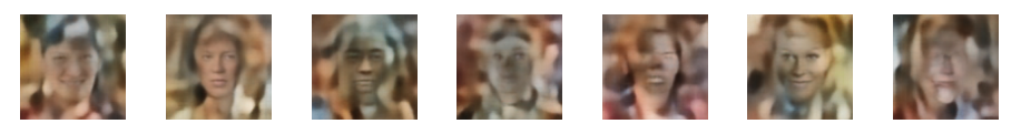
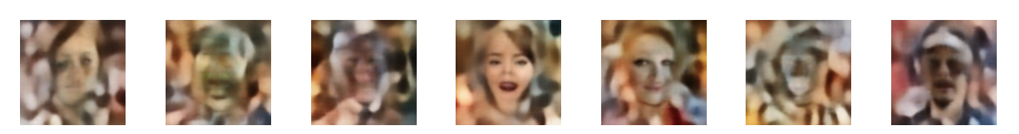
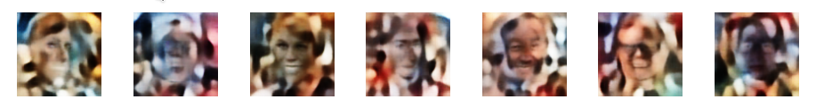
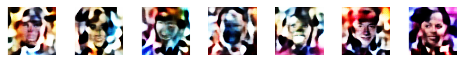
Then I fed these arbitrary z-points into the Decoder. Below you see the results after 10 training epochs of the AE; I selected only 10 of 100 data points created for each value of boundary (the images all look more or less the same regarding the absence or blurring of clear face contours):
boundary = 0.5
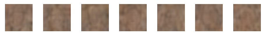
boundary = 2.5
boundary = 5.0
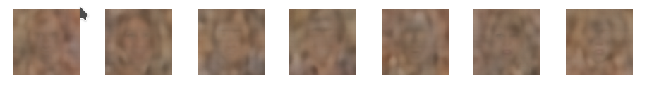
boundary = 8.0
boundary = 10.0
boundary = 15.0
boundary = 20.0
boundary = 30.0
boundary = 50
This is more a collection of face hallucinations than of usable face images. (Interesting for artists, maybe? Seriously meant …).
So, most of the points in the latent space of an Autoencoder do NOT represent reasonable faces. Sometimes our random selection came close to a region in latent space where the result do resemble a face. See e.g. the central image for boundary=10.
From the images above it becomes clear that some arbitrary path inside the latent space will contain more points which do NOT give you a reasonable face reproduction than points that result in plausible face images – despite a successful training of the Autoencoder.
This result supports the impression that the latent space of well trained Autoencoders is almost unusable for creative purposes. It also raises the interesting question of what the distribution of “meaningful points” in the latent space really looks like. I do not know whether this has been investigated in depth at all. Some links to publications which prove a certain scientific interest in this question are given in the last section of this posts.
I also want to comment on an article published in the Quanta Magazine lately. See “Self-Taught AI Shows Similarities to How the Brain Works”. This article refers to “masked” Autoencoders and self-supervised learning. Reconstructing masked images, i.e. images with a superposition of a mask hiding/blurring pixels with a reasonably equipped Autoencoder indeed works very well. Regarding this point I totally agree. Also with the term “self-supervised learning”.
But to suggest that an Autoencoder with this (rather basic) capability reflects methods of the human brain is in my opinion a massive exaggeration. On the contrary, in my opinion an AE reflects a dumbness regarding the storage and usage of otherwise well extracted feature patterns. This is due to its construction and the nature of its mapping of image contents to the latent space. A child can, after some teaching, draw characteristic features of human faces – out of nothing on a plain white piece of paper. The Decoder part of a standard Autoencoder (in some contrast to a GAN) can not – at least not without help to pick a meaningful point in latent space. And this difference is a major one, in my opinion.
A first interpretation – the curse of many dimensions of the latent space
I think the reason why arbitrary points in the multi-dimensional latent space cannot be mapped to images with recognizable faces is yet another effect of the so called “curse of high dimensionality”. But this time also related to the latent space.
A normal Autoencoder (i.e. one without the Kullback-Leibler loss) uses the latent space in its vast extension to produce points where typical properties (features) of faces and background are encoded in a most unique way for each of the input pictures. But the distinct volume filled by such points is a pretty small one – compared to the extensions of the high dimensional latent space. The volume of data points resulting from a mapping-transformation of arbitrary points in the original feature space to points of the latent space is of course much bigger than the volume of points which correspond to images showing typical human faces.
This is due to the fact that there are many more images with arbitrary pixel values already in the original feature space of the input images (with lets say 30000 dimensions for 100×100 color pixels) than images with reasonable values for faces in front of some background. The points in the feature space which correspond to reasonable images of faces (right colors and dominant pixel values for face features), is certainly small compared to the extension of the original feature space. Therefore: If you pick a random point in latent space – even within a confined (but multidimensional) volume around the origin – the chance that this point lies outside the particular volume of points which make sense regarding face reproduction is big. I guess that for z_dim > 200 the probability is pretty close to 1.
In addition: As the mapping algorithm of a neural Encoder network as e.g. CNNs is highly non-linear it is difficult to say how the boundary hyperplanes of mapping areas for faces look like. Complicated – but due to the enormous number of original images with arbitrary pixel values – we can safely guess that they enclose a rather small volume.
The manifold of data points in the z-space giving us recognizable faces in front of a reasonably separated background may follow a curved and wiggly “path” through the latent space. In principal there could even be isolated unconnected regions separated by areas of “chaotic reconstructions”.
I think this kind of argumentation line holds for standard Autoencoders and variational Autoencoders with a very small KL loss in comparison to the reconstruction loss (BCE (binary cross-entropy) or MSE).
Why do Variational Autoencoders [VAEs] help?
The fist point is: VAEs reduce the total occupied volume of the latent space. Due to mu-related term in the Kullback-Leibler loss the whole distribution of z-points gets condensed into a limited volume around the origin of the latent space.
The second reason is that the distribution of meaningful points are smeared out by the logvar-term of the Kullback-Leibler loss.
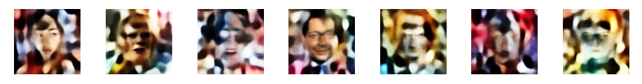
Both effects enforce overlapping regions of meaningful standard Gaussian-like z-point distributions in the latent space. So VAEs significantly increase the probability to hit a meaningful z-point in latent space – if you chose points around the origin within a distance of “1” per coordinate (or vector component).
The total distance of a point and its vector in z-space has to be measured with some norm, e.g. the Euclidian one. Actually we should get meaningful reconstructions around a multidimensional sphere of radius “16”. Why this is reasonable will be discussed in forthcoming posts.
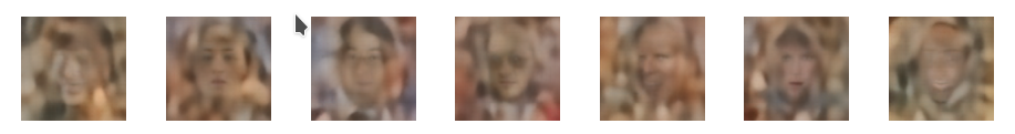
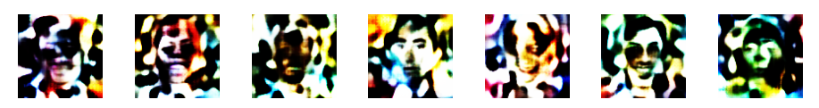
Please, also look at the series on the technical realization of VAEs in this blog. The last posts there prove the effects of the KL-loss experimentally for Celeb A data. Below you find a selection of images created from randomly chosen points in the latent space of a Variational Autoencoder with z_dim=200 after 10 epochs.

Conclusion
Enough for today. Whilst standard Autoencoders solve certain tasks very well, they seem to produce very specific data distributions in the latent space for CelebA images: Only certain regions seem to be suitable for the reconstruction of “meaningful” images with human faces.
This problem may have its origin already in the feature space of the original images. Also there only a small minority of points represents humanly interpretable face images. This becomes obvious when you look at the vast amount of possible pixel values in a feature space of lets say 96x96x3 = 27,648. Each of these dimension can get a value between 0 and 255. This gives us more than 7 million combinations. Only a tiny fraction of these possible images will show reasonable faces in the center with a reasonably structured background around.
From a first experiment the chance of hitting a data point in latent space which gives you a meaningful image seems to be small. This result appears to be a variant of the curse of high dimensionality – this time including the latent space.
In a forthcoming post
Autoencoders, latent space and the curse of high dimensionality – II – a view on fragments and filaments of the latent space for CelebA images
we will investigate the z-point distribution in latent space with a variety of tools. And find that this distribution is fragmented and that the z-points for CelebA images are arranged in certain regions of the latent space. In addition we will get indications that the distribution contains filament-like structures.
Links
https://towardsdatascience.com/ exploring-the-latent-space-of-your-convnet-classifier-b6eb862e9e55
Felix Leeb, Stefan Bauer, Michel Besserve,Bernhard Schölkopf, “Exploring the Latent Space of Autoencoders with
Interventional Assays”, 2022,
https://arxiv.org/abs/2106.16091v2 // https://arxiv.org/pdf/2106.16091.pdf
https://wiredspace.wits.ac.za/ handle/10539/33094?show=full
https://www.elucidate.ai/post/ exploring-deep-latent-spaces
Books:
T. Rashid, “GANs mit PyTorch selbst programmieren”, 2020, O’Reilly, dpunkt.verlag, Heidelberg, ISBN 978-3-96009-147-9
D. Foster, “Generatives Deep Learning”, 2019, O’Reilly, dpunkt.verlag, Heidelberg, ISBN 978-3-96009-128-8