This post series is about creative abilities of convolutional Autoencoders [AE] which have been trained on a set of human face images. The objectives of this series and its numerical experiments are:
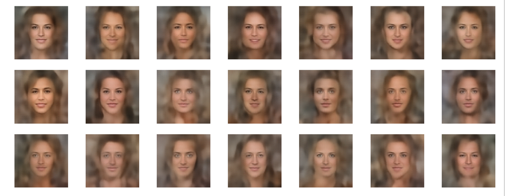
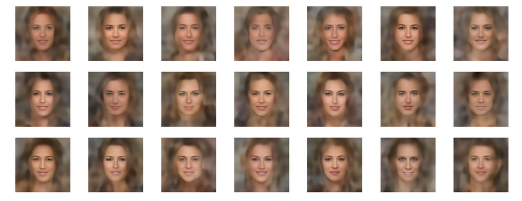
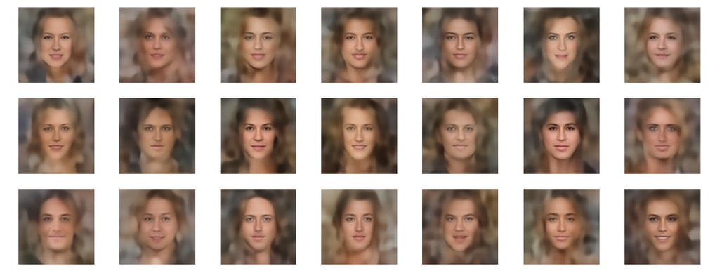
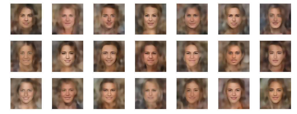
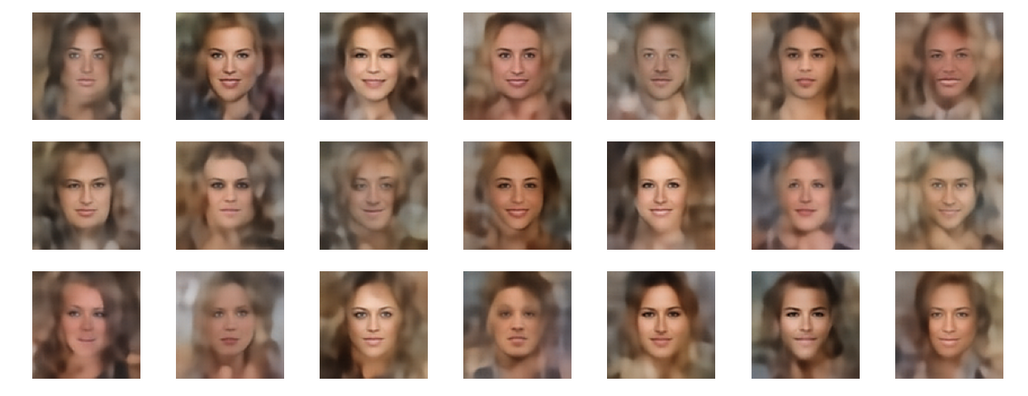
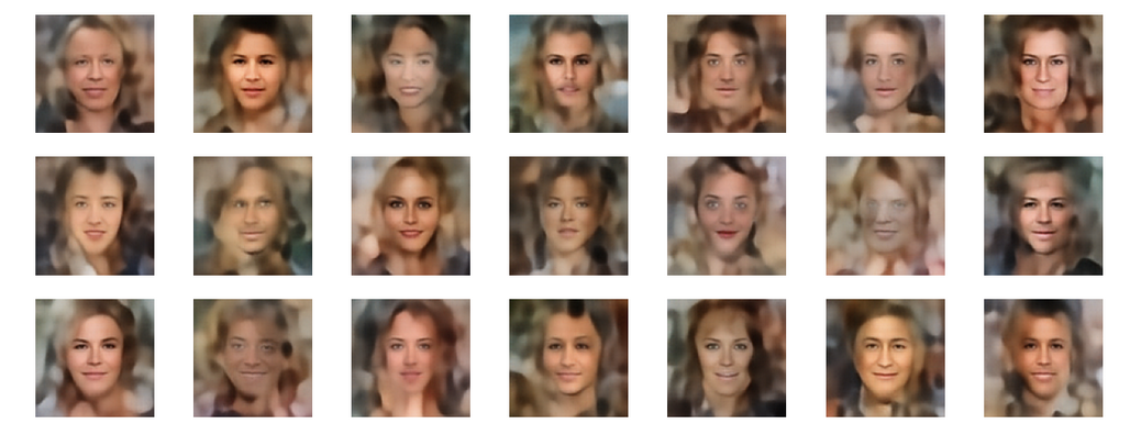
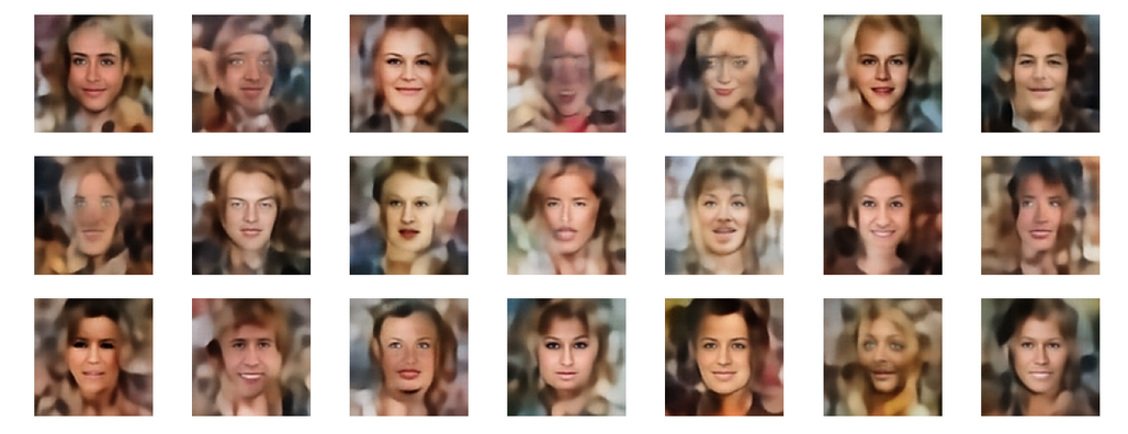
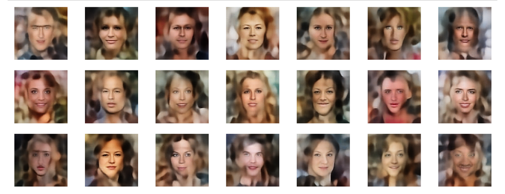
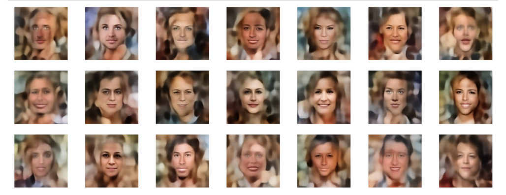
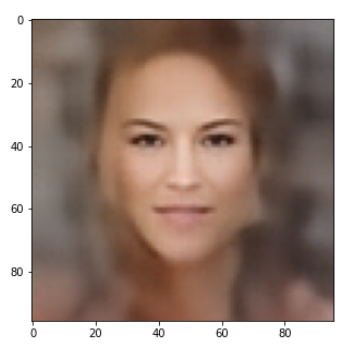
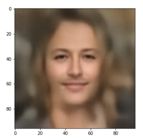
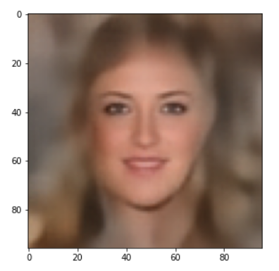
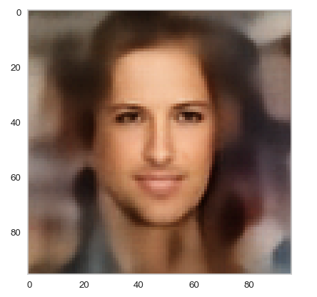
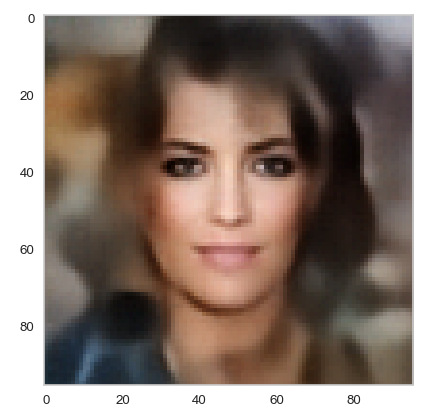
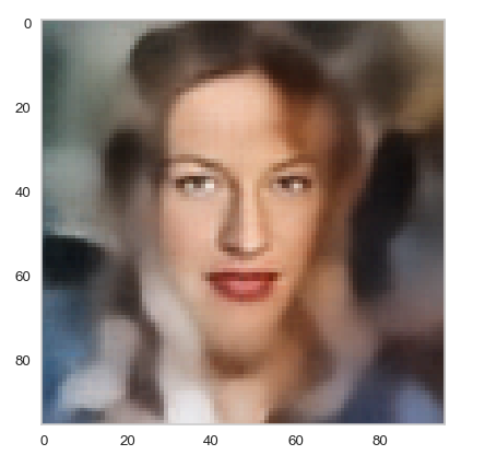
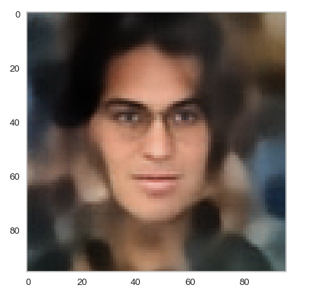
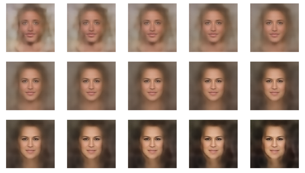
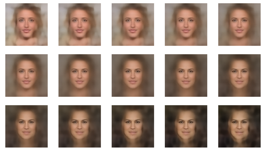
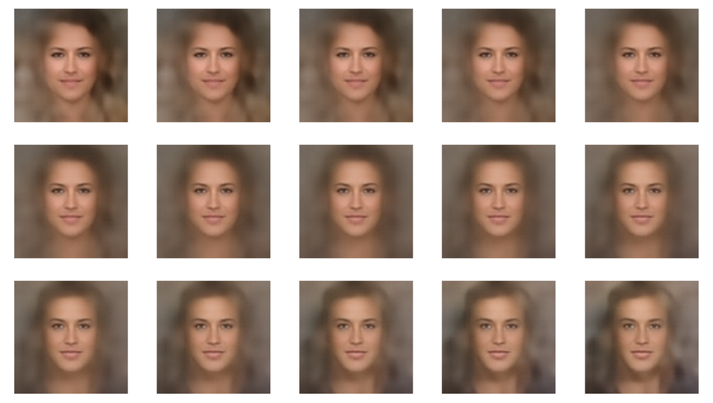
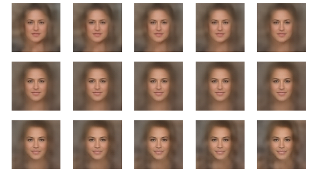
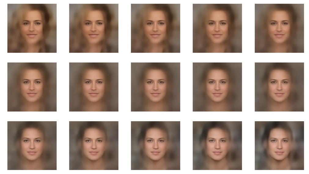
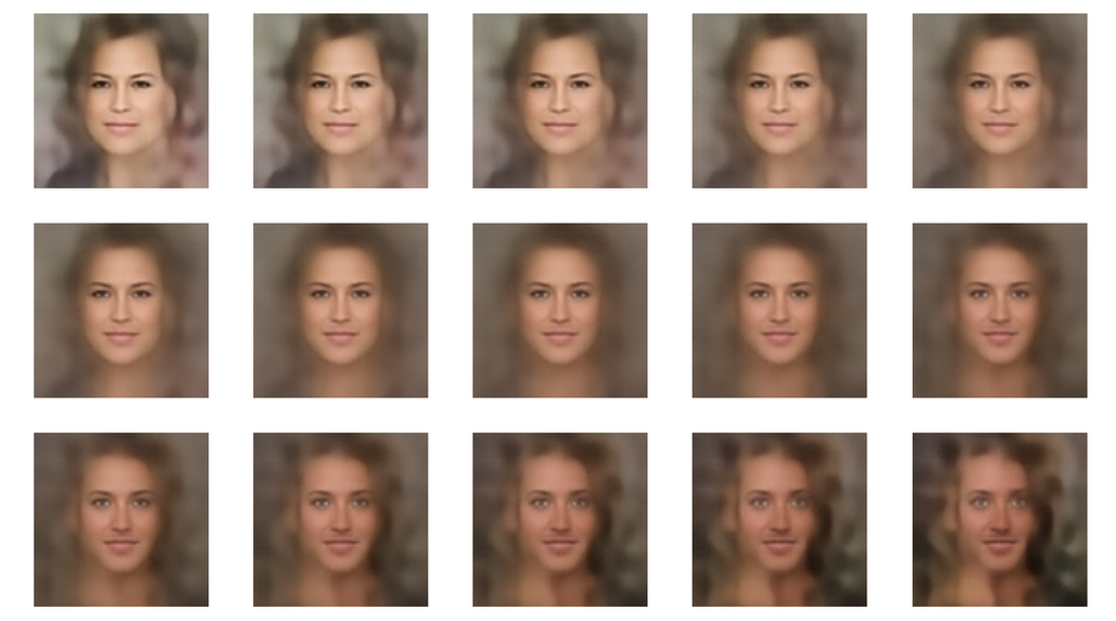
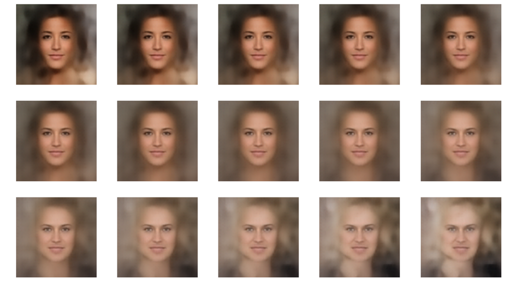
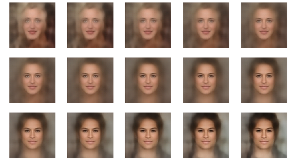
- We want to create images with human faces from statistical z-vectors and related z-points in the AE’s latent space [z-space or LS]. Image creation will be done with the help of the AE’s Decoder after a training on the CelebA dataset.
- We work with a standard Autoencoder, only. I.e., we do NOT add any artificial layers and cost terms to the Autoencoder’s layer structure (as it is done e.g. in Variational Autoencoders).
- We analyze the position, shape and internal structure of the multidimensional z-vector distribution created by the AE’s Encoder after training. We assume that generated statistical z-vectors must point to respective regions of the latent space to guarantee images with reasonable content.
- We raise the question whether simple statistical generator algorithms are sufficient to cover these regions with statistical z-vectors.
Our numerical experiments gave us some indications that such an endeavor is indeed feasible. In addition the third objective may give us some insight into the rules a trained AE follows when it encodes information about human faces into vectors of its latent space.
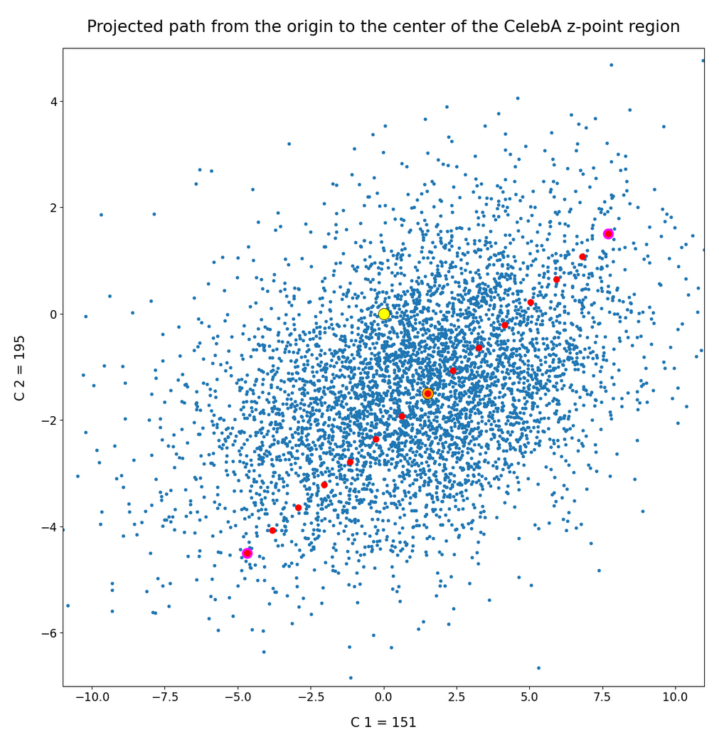
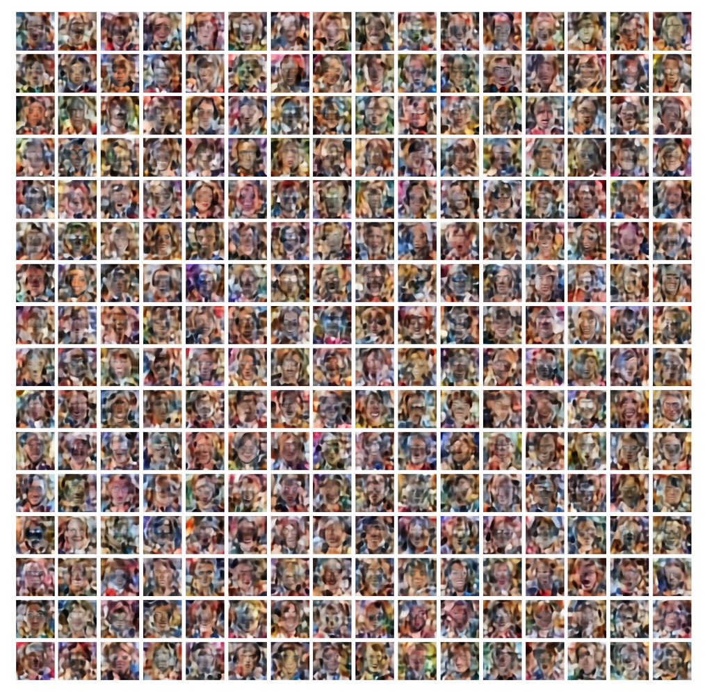
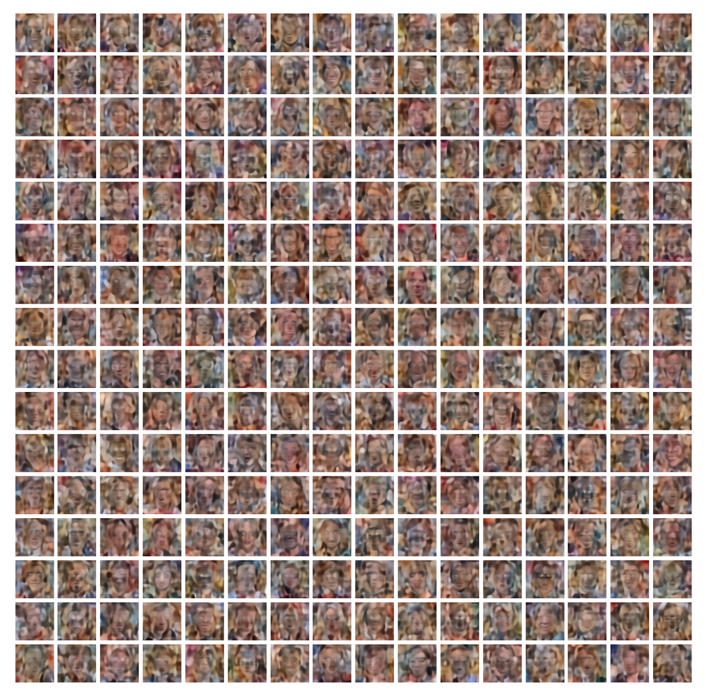
We have already studied the “natural” z-vector distribution created by a convolutional Autoencoder for CelebA images after a thorough training. The related z-point distribution fortunately filled just one confined and coherent off-center region of the AE’s latent space. Our experiments have furthermore shown that we must indeed restrict the statistical z-vector creation such that the vectors point to this particular region. Otherwise we will not get reasonable images. For details see the previous posts.
Autoencoders and latent space fragmentation – VII – face images from statistical z-points within the latent space region of CelebA
Autoencoders and latent space fragmentation – VI – image creation from z-points along paths in selected coordinate planes of the latent space
Autoencoders and latent space fragmentation – V – reconstruction of human face images from simple statistical z-point-distributions?
Autoencoders and latent space fragmentation – IV – CelebA and statistical vector distributions in the surroundings of the latent space origin
Autoencoders and latent space fragmentation – III – correlations of latent vector components
Autoencoders and latent space fragmentation – II – number distributions of latent vector components
Autoencoders and latent space fragmentation – I – Encoder, Decoder, latent space
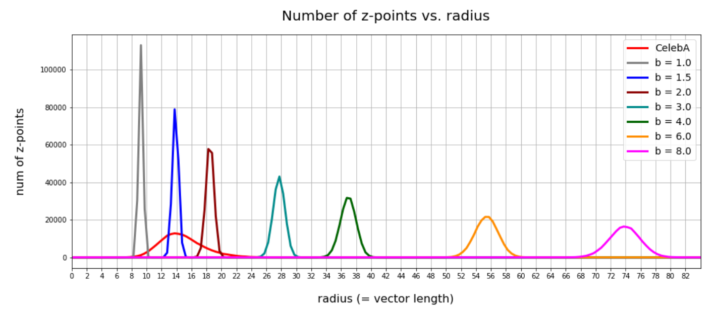
The frustrating point so far was that simple methods for creating statistical vectors fail to put the end-points of the z-vectors into the relevant latent space region. In particular methods based on constant probability distributions within a common value interval for all z-vector components are doomed to miss the interesting region due to intricate mathematical reasons.
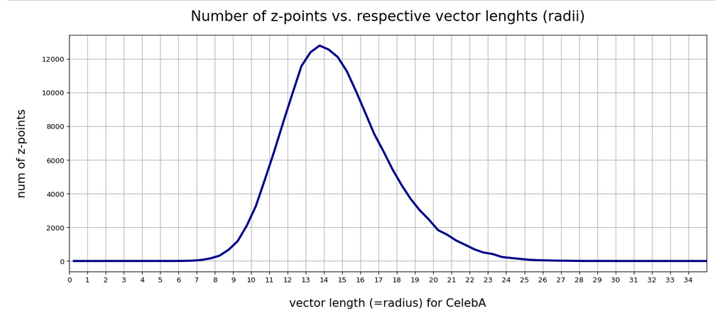
Afterward we tried to restrict the component values of test vectors to intervals defined by the shape of the number distribution for the values of each component of the CelebA related z-vectors. Such a distribution is nothing else than a one-dimensional probability density function for our special set of encoded CelebA samples: The function describes the probability that a component of a z-vector for human face images gets a value within a certain small value range. The probability distributions for all z-vector components were bell shaped and showed clear transitions to flat wings with very low values. See the plots below. This allowed us to define a value range
d_j_l < x_j < d_j_h
for each vector component x_j.
But keeping statistical values per component within the identified respective interval was not a sufficient restriction. We saw this clearly in the last post from significant irregular fluctuations in the reconstructed images. Obviously the components of statistically generated z-vectors must in addition fulfill correlation conditions.
The questions which I want to answer in this post are:
- Can we approximate the 1-dimensional probability density functions for the z-vector components by some simple and common mathematical function?
- What kind of correlations do we find between the components of the z-vectors encoding the information of human face images?
- Can we derive some mathematical description of the multivariate z-vector distribution created by convolutional AEs for human face images in the AE’s multidimensional latent space?
Correlations are to be expected …
Please note: We deal with a multidimensional problem. A single latent vector encodes information about a human face image via all of its component values and by relations between these values. Regarding the purpose and the task an AE has to fulfill, it would be naive to assume that the components of our multi-dimensional z-vectors were independently organized. A z-vector encodes information for a convolutional Decoder to combine patterns detected by the Encoder and represented in neural (feature) maps of the networks to create an image. This is a subtle business. Just think about what you do when you draw a sketch of a human face. There are a lot of rules you follow.
When you think about the properties of basic feature patterns in a human face you would certainly assume that the pixel data of a corresponding image show strong correlations. This is among other things due to obvious symmetries – not excluding fluctuations of basic parameters describing human face features. But a nose tends to be at a position below the eyes and at a mid-distance of the eyes. In additions fluctuations of face features would on average respect certain limits given by natural proportions of a face. It would therefore be unreasonable to assume that the input for a Decoder to create a superposition of elementary patterns consists of un-correlated data. Instead the patterns in the original data should not only lead to well adjusted weights in the convolutional networks’ feature maps, but also to well regulated structural elements in the data distribution in the target space of the information encoding, namely in the latent space.
If the relations of the vector components were of a complex, highly non-linear kind and involved many dimensions at the same time we might be lost. But the results we have gained so far indicate a proper common structure of at least the density function for the individual components. This gives us some hope that the multidimensional problem somehow involves well defined 1-dimensional constituents. Whether this a sign that the multidimensional structure of the z-vector distribution can be decomposed into low-dimensional relations remains to be seen.
Observations regarding the z-vector distribution created by convolutional Autoencoders for human face images
Coordinate values of the z-points are identical to z-vector component values when we fix the end of each vector to the origin of the latent space coordinate system. The z-vector distribution thus directly corresponds to a z-point density distribution in the orthogonal coordinate system of the AE’s multi-dimensional LS. We have already made three interesting observations regarding these distributions:
- The individual probability density function for a selected component of the latent vectors has a bell-shaped form. One , therefore, is tempted to think of a Gaussian function. This would indicate a possible normal distribution for the coordinate values of the z-points along each of the selected coordinate axes.
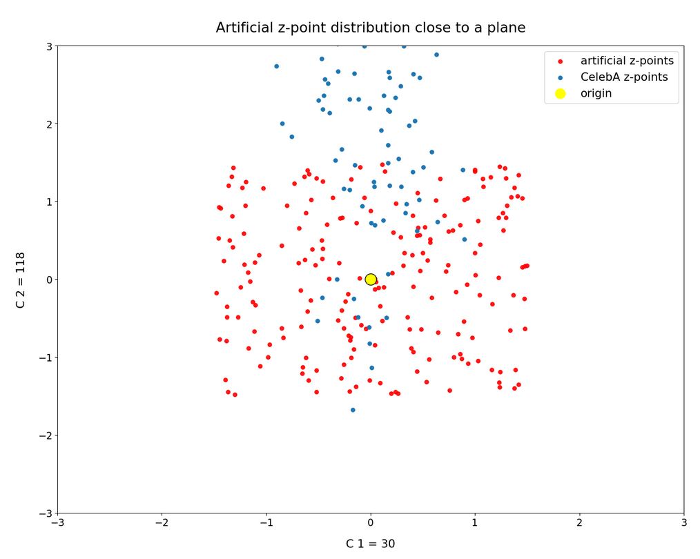
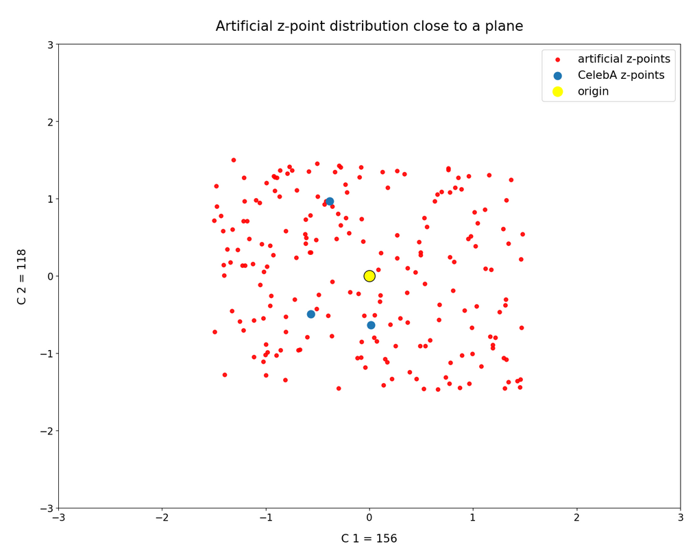
Note: This does not exclude that the probability distributions for the components are correlated in some complex way. - When we plotted the projection of the z-point distribution onto 2-dimensional coordinate planes (for selected pairs of coordinate axes) then almost all of the resulting 2-dimensional density distributions seemed to have a defined core with an ellipsoidal form of its boundary.
- For certain component- or axis-pairs the main axes of the apparent ellipses for pair-wise density function appeared rotated against the coordinate axes. The elongated regular and more or less symmetric forms showed a diagonal orientation (with different angles). This alone signals a strong correlation between related two vector components. Indeed we found high values for certain elements of the matrix of normalized Pearson correlation coefficients for the multi-dimensional distribution of z-vector component values.
These observations are not unrelated; they indicate a clear pattern of dependencies and correlations of the distributions for the variables in place. Regarding the data basis we have to keep five things in mind:
- We treat the z-point distribution for CelebA images as a multi-dimensional probability density distribution. During the analysis we look in particular at 2-dimensional projections of this distribution onto planes spanned by a selected pair of orthogonal axes of the LS coordinate system. We also consider the one-dimensional value distributions for z-vector components. In this sense we regard the z-vector components as logically separate variables.
- The data used are numbers of z-points counted in finite 1d-intervals, 2d-rectangles or multidimensional cuboids. We fit idealized functions to the respective discrete bar plots. Even if there is a good 1d-fit fluctuations may especially get visible in multidimensional plots for correlated data. A related probability density requires a normalization. We drop the resulting constant factors in the qualitative discussions below.
- Statistical (un-)correlation of statistical variable distributions must NOT to be confused with underlying variable (in-) dependency. Linear correlations can be reduced to zero by coordinate transformations without eliminating the original variable dependencies.
- Pearson correlation coefficients are sensitive to linear elements in the relations of logically separate variable distributions. They can not fully cover non-linear distribution relations or covered variable dependencies.
- A transformation to a local coordinate system whose axes are aligned to the so called main axes of the multidimensional distributions does not remove the original data relations – but there may exist a coordinate system in which the distribution data can be described in a simple, factorized form corresponding to a composition of seemingly un-correlated data distributions.
Anyway – by discussing density distributions we work on overall and large scale average relations between statistical value distributions for our variables, namely the z-vector components. We do not cover local micro-relations that may be in place in addition.
The relation of ellipses with Gaussian probability densities
Probability density functions for two logically separate, but maybe not un-correlated variables have to be multiplied. In our case this reflects the following point: First we determine the probability that the value of component x_i lies in a certain (infinitesimal) interval and then we determine the probability that (for the given value of x_i) the component x_j falls into another value range. The distributions for a specific variable can include variable relations and thus the probability density g(x_j) can include a dependency g(x_j(x_i)).
In the case of uncorrelated normal distributions per coordinate we can just multiply the individual Gaussians g(x_i) * g(x_j). Due to the quadratic terms in the exponent of the Gaussians we then get a sum of quadratic expressions in the common exponent, having the form fac1 * (x_i-mu_i)**2 + fac2 * (x_j-mu_j)**2.
By setting this expression to a constant value we get contour lines of the probability density distribution for the (x_i, x_j)-distribution. Quadratic sums correspond to the definition of an ellipse having main axes which are aligned with the x_i- and x_j-axes of the coordinate system. Thus the contour lines of a 2-dimensional distribution composed of un-correlated Gaussians are ellipses having an orientation aligned with the coordinate axes.
This was for un-correlated density-distributions of two vector components. Mathematically a linear correlation between a pair of Gaussians-distributions corresponds to an affine transformation of the contour-ellipses. The transformation can be expressed by a defined sequence of matrix operations describing a translation, rotations (in a defined order) and a dilation.
This means: The contour lines for a 2-dimensional probability density composed of linearly correlated Gaussians are still ellipses. But these ellipses will appear to be shifted, rotated and stretched along the main axes in comparison with their originally un-correlated Gaussian counterparts. The angle of rotation depends on details of the correlation function and the original standard deviations. The Pearson correlation matrix for linearly correlated distributions is a positive-definite one and, of course, shows off-diagonal elements different from zero. This result can be extended to multivariate normal distributions in spaces with many dimensions and related affine transformations of the coordinate system.
A multivariate normal distribution with linear correlations between the Gaussians results in elliptic contour lines for pair-wise density distributions in the respective 2D-coordinate planes of an orthogonal coordinate system. When we define the contours via multiples of the standard deviations of the underlying Gaussian functions we arrive at so called confidence ellipses.
A really nice mathematical aspect is that the basic parameters of the confidence ellipses can be derived from the normalized correlation coefficients of the Pearson matrix of the multivariate probability distribution. I will come back to this point in forthcoming posts in more detail. For now we just need to know that a multidimensional probability density comes along with confidence ellipses which can be calculated with the help of Pearson correlation coefficients.
Before we go on a word of caution: For a general multi-variate distribution it is not at all clear that it should decompose into a factorized form. However, for a multivariate normal distribution with un-correlated or only linearly correlated components this is by definition different. In this case a transformation to a coordinate system can be found which leads to a complete decomposition into a product of (seemingly) un-correlated Gaussians per component. The latter point lies at the center of PCA and SVD algorithms, which diagonalize the Pearson correlation matrix.
Do we really have Gaussian probability distributions for the individual z-vector-components?
After this short tour into the world of (multi-variate) normal distributions, Gaussian functions and related ellipses we are a bit better equipped to understand the density distributions in the latent space of our Autoencoders for human face images.
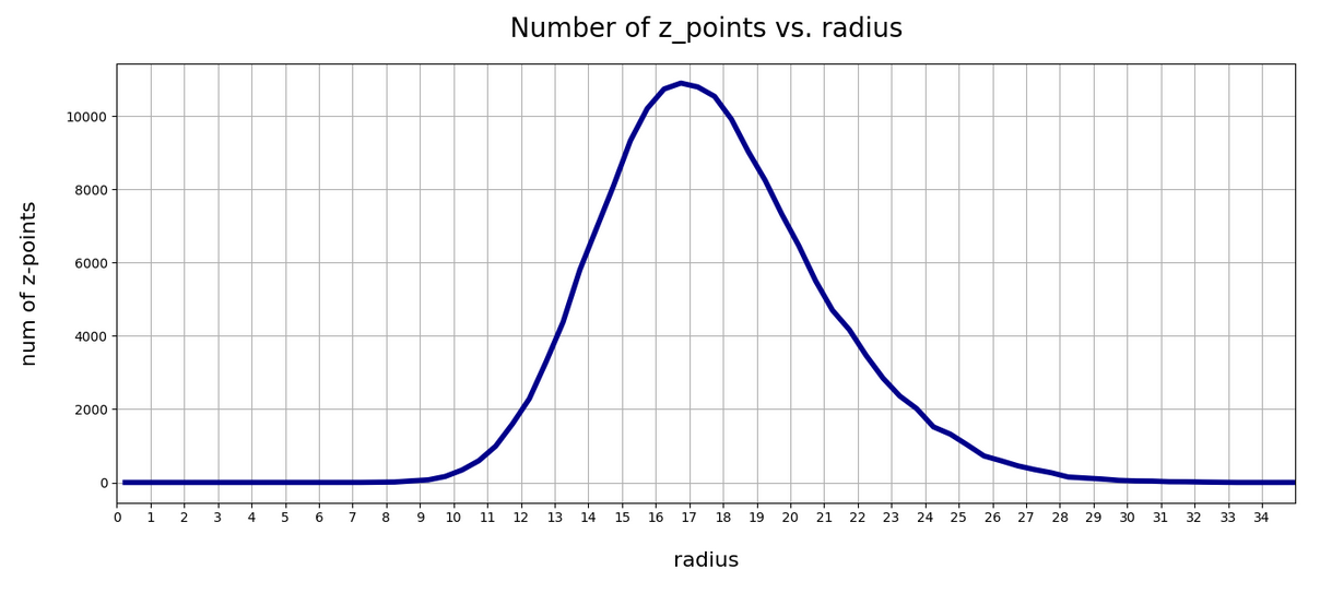
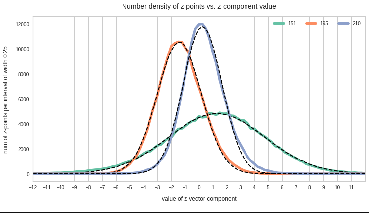
Let me remind you about the shapes of the number distribution for our concrete z-vector components resulting for for CelebA face images. The first plot shows the number densities on sampling intervals of width 0.25 for selected vector components resulting for case I of our experiments. The second plot shows the number densities for the values of selected components of case II.
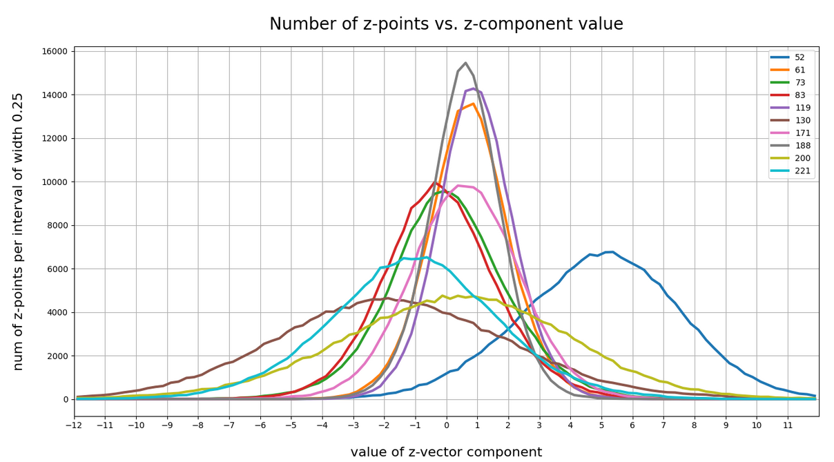
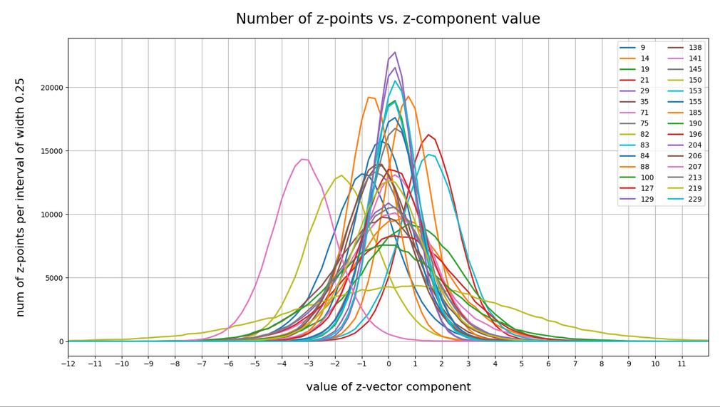
Ok, these curves do resemble Gaussians and some fluctuations are normal. But can we prove the Gaussian properties of the curves a bit better?
Well, for case II I have drawn the best fits by Gaussian functions with the help of SciPy’s optimize.curve_fit() for 3 and yet another 4 selected components of the latent vectors and the respective number distribution curves. The dashed lines show the approximations by Gaussian functions:
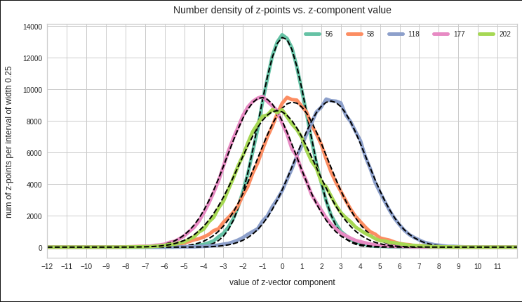
The selected components are part of the list of around 20 dominant component distributions – due to their relatively large standard deviations. But the Gaussian form is consistently found for all components (with some small deviations regarding the symmetry of the curves).
So all in all it looks like as if our convolutional AE has indeed created a multivariate normal z-point distribution in the latent space. As said: This does not exclude correlations …
Pairwise linear correlations of the (normal) probability distributions for the latent vector components?
Now we are a bit bold – and assume the best case for us: Could the approxiate Gaussians distributions for the component values be pair-wise and linearly correlated? What would be a clear indication of a pair-wise linear correlation of our component distributions?
Well, we should find an elliptic form of contour lines in the 2-dimensional distribution for the component pair in the respective coordinate plane of the basic orthogonal LS coordinate system. This imposes quite strong symmetry conditions on the contour lines. The ellipses can be shifted and rotated – but they should remain being ellipses. If non-linear contributions to the correlation had a significant impact this would not be the case.
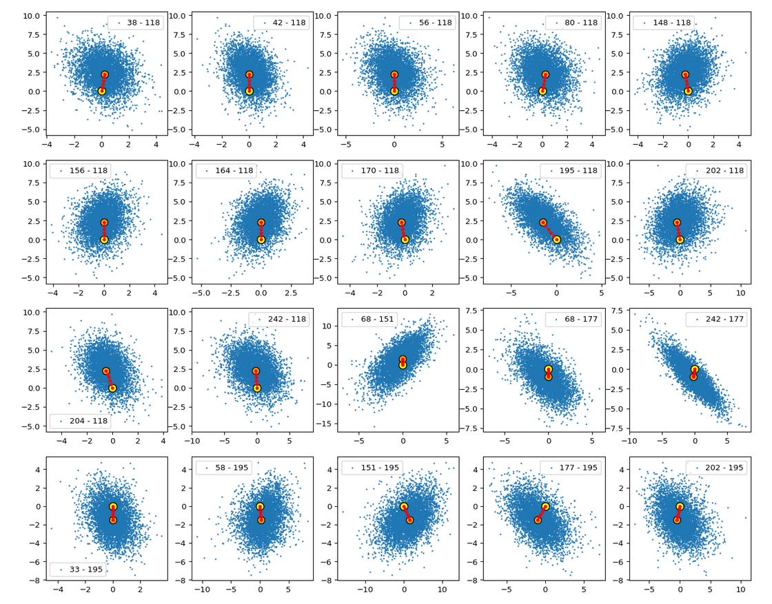
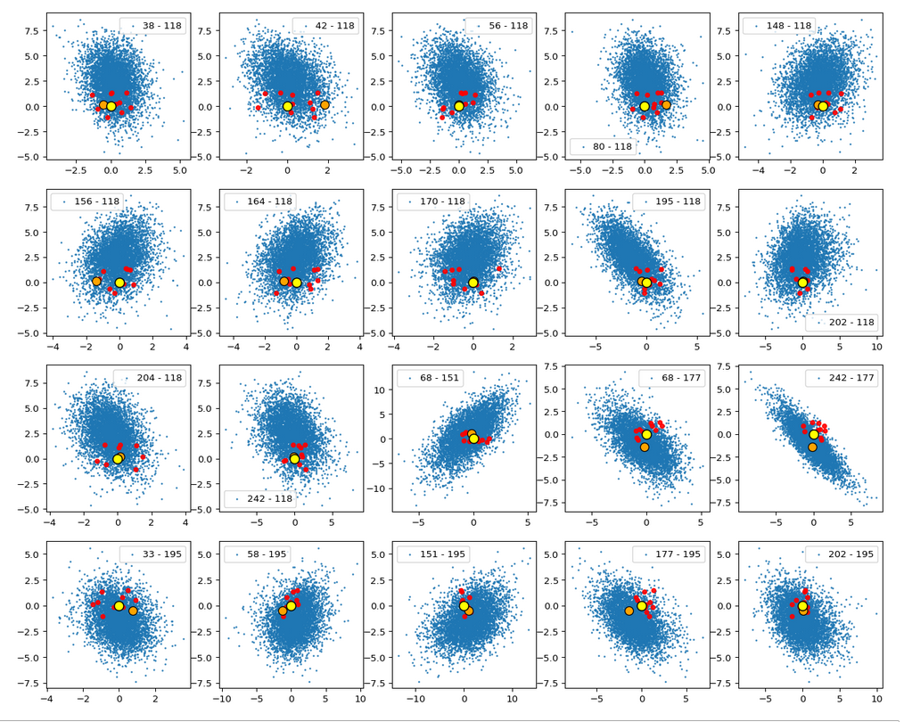
Practically it is not trivial to prove that we have approximately rotated ellipses in 2 dimensions. Satter plos alone do not help: Ellipses fit a lot of plotted distributions of discrete data points quite well. We really need to count number densities to get reliable contour lines. The following plots show such contour lines based on number sampling in rectangles and local smoothing operations with the help of scipy.stats.gaussian_kde().
The fat red and dark orange lines show corresponding confidence ellipses derived from the original CelebA distribution. See below for some remarks on confidence ellipses.
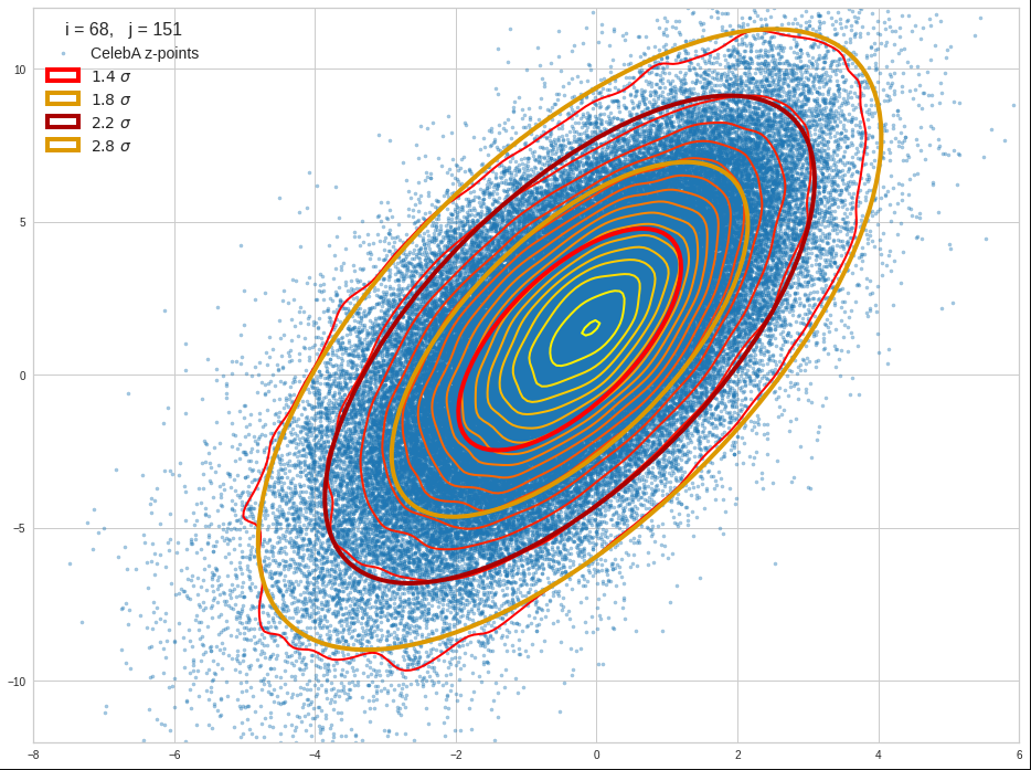
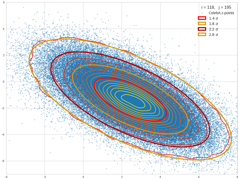
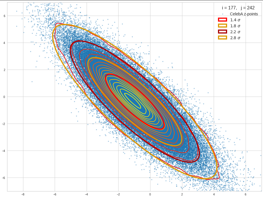
The contours are basically of elliptic shape although they do not show the complete symmetry expected for pure and linearly dependent Gaussian distributions. But overall the confidence ellipses fit quite well into the general form and orientation of the distributions. We also see that for higher σ-levels the coincidence with nearby contours is quite good. The wiggles in the contour change with the z-vector selection a bit.
We conclude that our basic impression regarding an elliptic shape of the z-point distributions is basically consistent with only linearly correlated Gaussian probability density distributions for the component values of the latent vectors.
Approximation of the core of the multivariate z-point distribution by confidence ellipses for component pairs
Above I referred to the boundary of a core of the probability density for two selected vector components. But how would we define the “boundary” of a continuous distribution in the coordinate planes? Answer: As we like – but based on the decline of the approximate Gaussian curves.
We can e.g. pick two times the half-width in each direction or we can use contours defined by confidence levels.
For 2 ≤ fact * σ ≤ 3 we saw already that the contour lines could well be fitted by confidence ellipses. A 3-sigma level covers around 97% of all data points or more. A 2 sigma-level ellipse encircles between 70% and 90% of all data points, depending on the eccentricity of the ellipse. Note that the numbers are smaller for ellipses than for rectangles. I.e. the standard 68-95-99.7 rule does not apply.
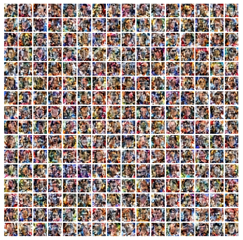
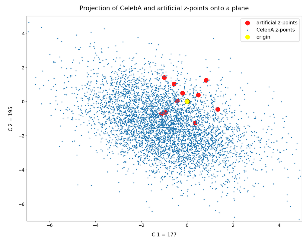
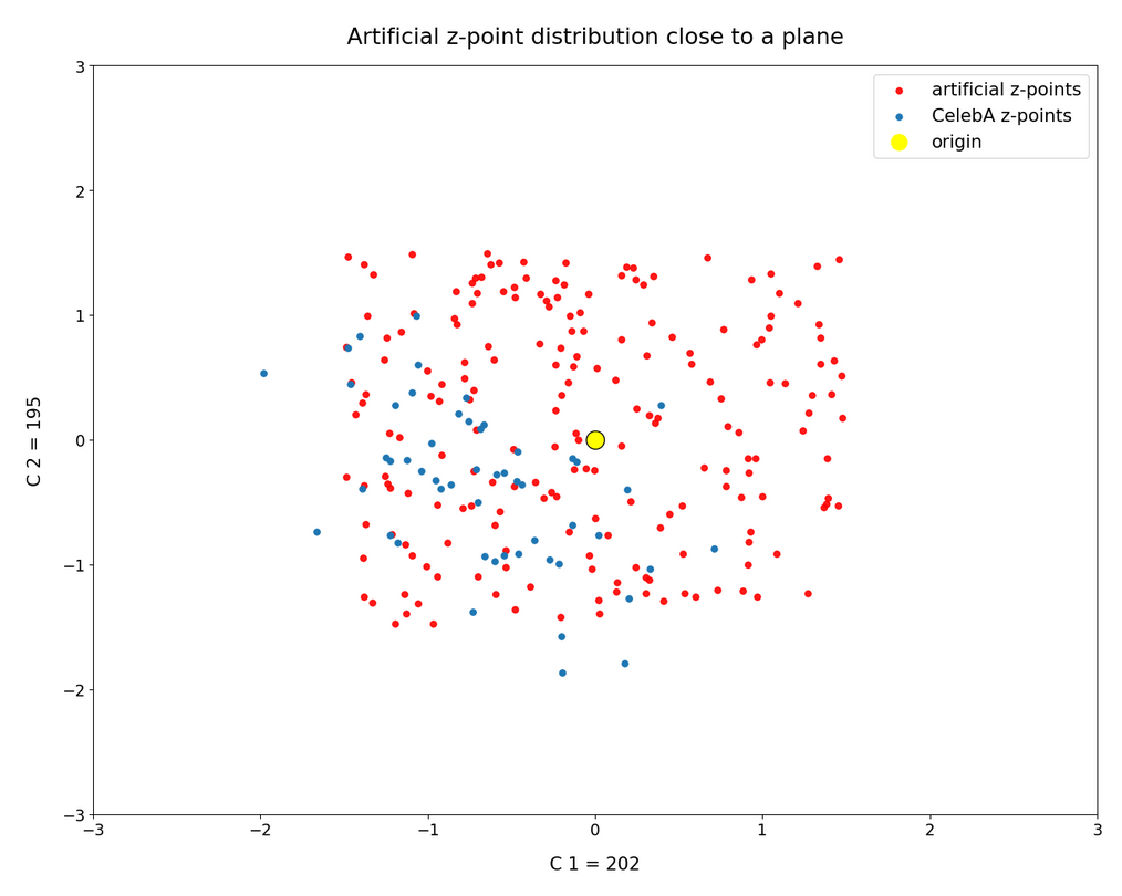
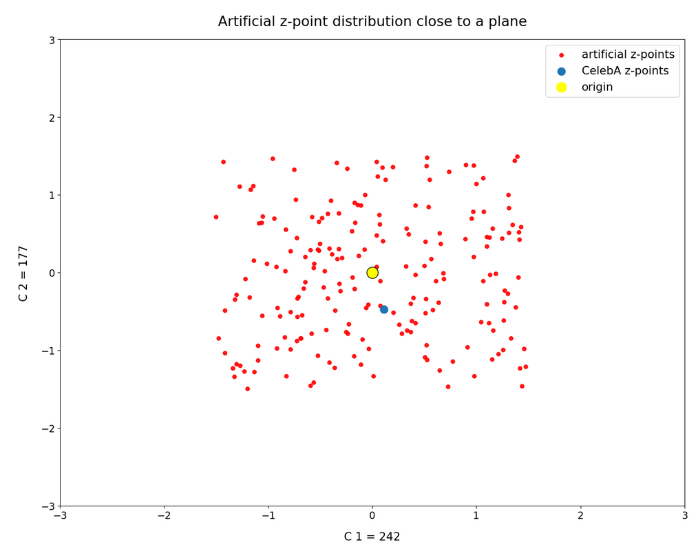
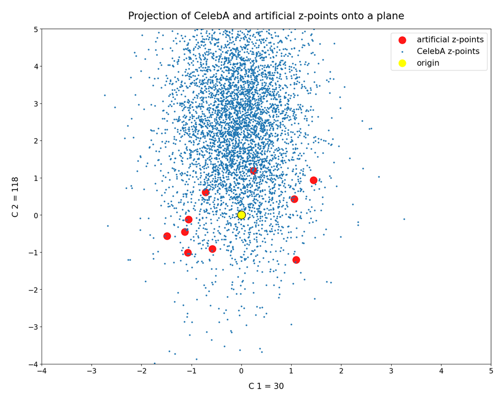
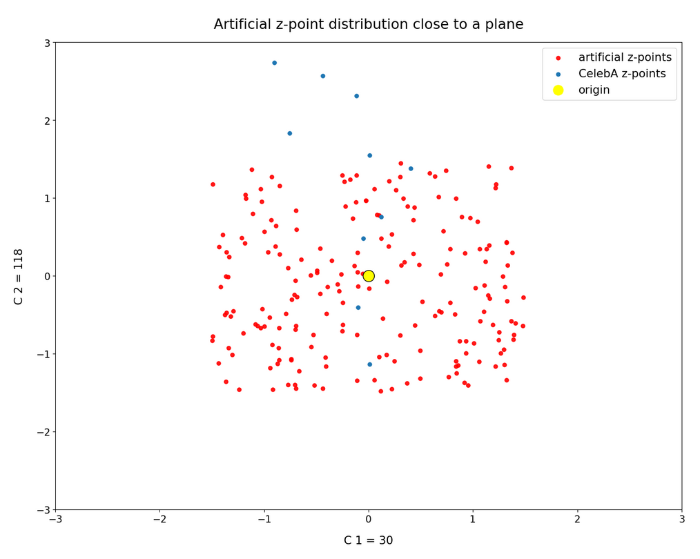
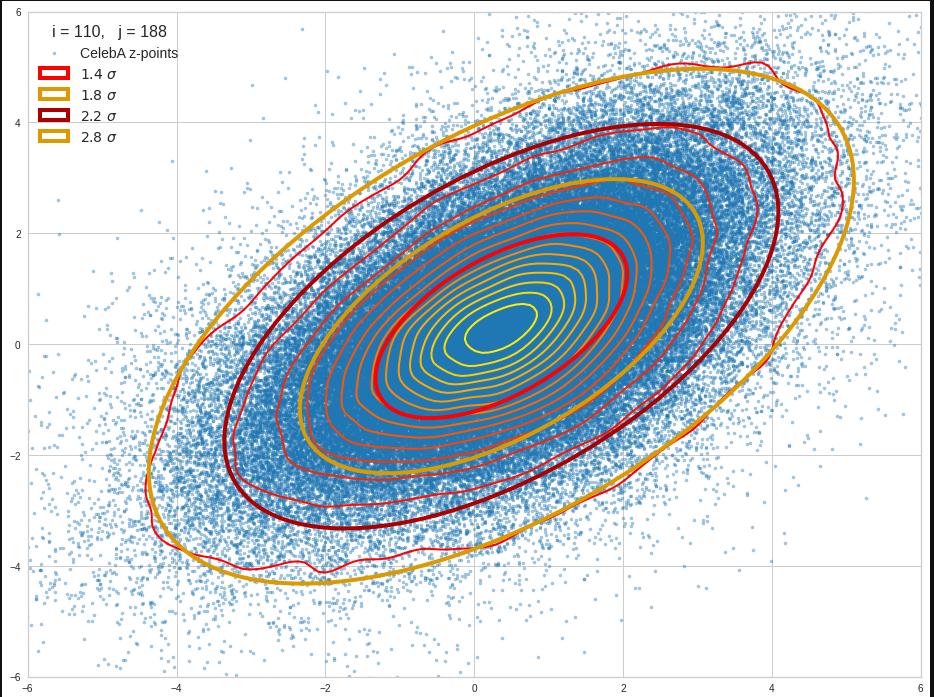
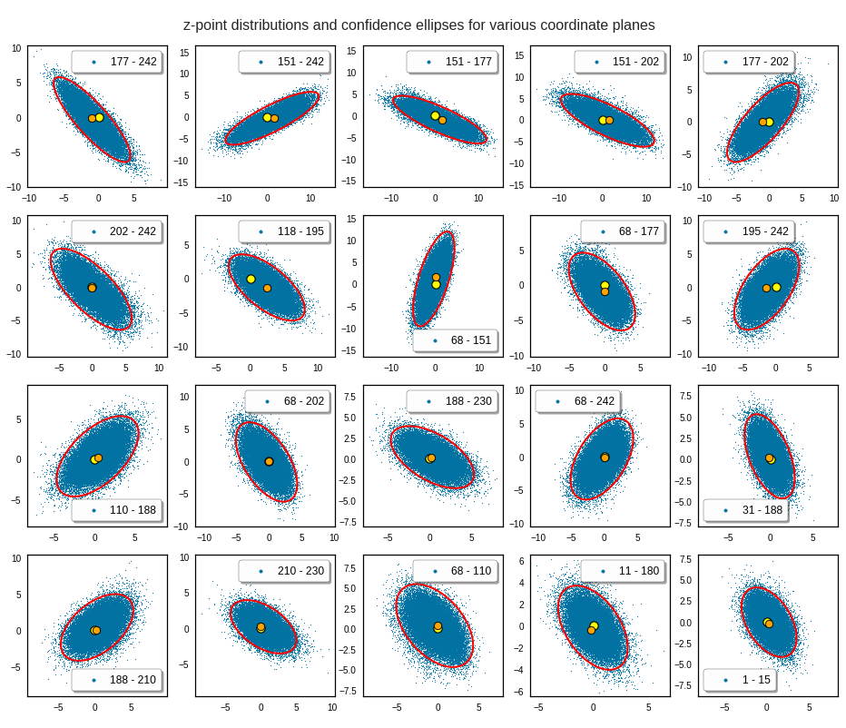
The plots below give you an impression of how well ellipses for a 2σ-confidence level approximate the core of the CelebA distribution in selected 2D coordinate planes of the latent space:
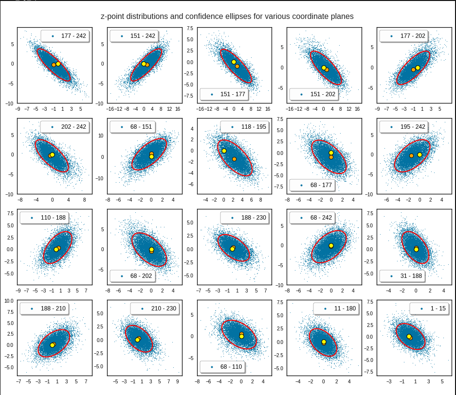
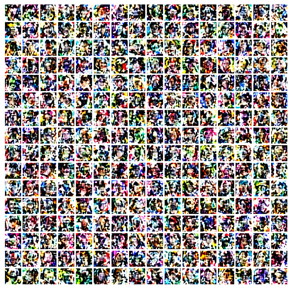
Each of the sub-plots was based on 10,000 statistically selected vectors of the 170,000 available in my test runs. This is a relative low number. Therefore, for a certain diameter of the points in the scatter plot only the inner core appears to be densely populated. The next plots shows the results for a 3 σ-level of the ellipse – but this time for 50,000 vectors. With more vectors we could visually fill the outer regions of the core.
The orange points mark the center of the multidimensional distributions derived from the one-dimensional distribution curves for the components. We see that it does not always appear to be optimally centered. There are multiple reasons: Our functions are not fully symmetric as ideal Gaussians. And equally important: The accuracy of the position depends on the sampling resolution which was coarse. Outliers of the distribution do have an impact.
And how would we explain the appearance of Gaussians and ellipses?
This all looks quite good, despite some notable deviations regarding symmetry and maxima. Gaussians fit at least most of the important probability density curves very well, though not by a 100%. The appearance of an elliptic shape of the inner core of the distribution and the appearance of overall elliptic contour curves can be explained by linear correlations of the Gaussian distributions for the components.
The appearance of normal distributions per component and basically linear correlations is something that really should be explained. I mean, dwell a bit on what we have found:
A convolutional Autoencoder network with more than 10 million adjustable parameters encoded information about human face images in the form of a roughly multivariate normal distribution of z-points in its latent space – with basically linear correlations between the Gaussian curves describing the probability densities functions for the component values of the z-vectors.
I find this astonishing and not at all self-evident. It is one of the most simple solutions for a multidimensional situation one can imagine. The following questions automatically came to my mind:
Does such a result only appear for training images of defined objects with some Gaussian variation in their features? Are the normal distributions a reflection of variations of relevant features in the original data?
Is this a typical result for (convolutional) AEs? How does it depend on the dimensionality of the latent space? Does it automatically come with a large number of z-space dimensions? Is it an efficient way to encode feature differences in the latent space, which (convolutional) AEs in general tend to use due to their structure?
Do I personally have a convincing explanation? No. Especially not, as the data shown above stem from convolutional neural networks [CNNs] without any batch-normalization layers.
A first idea would be that the dominant features of a human face themselves show variations described by Gaussian normal distributions already in the original data and that convolutional filtering does not destroy such distributions during optimization. A problem of this idea lies in the (non-) linear activation functions used at the nodes of the neural maps. Though ReLU, Leaky ReLU and SeLU contain linear parts.
The other problem is the linear form of the correlations. This is a rather simple kind of correlations. But why should an AE choose this simple form into its mapping of image information to latent space vectors after training?
How to generate statistical vectors for the creation of human face images?
The positive message which comes with the above results is that our problem of how to create proper statistical z-vectors decomposes into a sequence of two-dimensional problems. We can use the data of the ellipses appearing in the density-distributions for pairs of vector components to confine the components of statistically generated z-vectors to the relevant region in the latent space. All ellipses together restrict the component values in a well defined form. In the next post I will shortly outline some methods of how we can use the information contained in the ellipses with available algorithms.
Conclusion
In this post we have seen that for the case of a convolutional Autoencoder trained on CelebA human face images the latent vector distributions showed some remarkable properties:
The probability density functions for all component values can roughly be approximated by Gaussian functions. The components appear to be pairwise linearly correlated – at least to first order analysis. This automatically implies elliptic contour curves for the pairwise number density functions of coordinate values. Such contour curves were indeed found with first order accuracy. The core of the probability density for the z-points in the latent space could therefore be approximated by confidence ellipses for a σ-level above σ = 2.5.
The elliptic conditions correspond to a multivariate normal distribution with linear correlations of the variables.
Before we get to enthusiastic about these findings we should be careful and await a further test. All statements refer to a first order approximations. A real multivariate normal distribution would decompose into un-correlated Gaussians and 2D-ellipses of probability densities of component pairs after a PCA transformation.
In the next post
I shall present the results of a PCA analysis. In later posts I will introduce a related method to restrict the components of statistical vectors to the relevant region in the latent space of our Autoencoder.
Links and literature
On first sight my short description of the relation between multivariate Gaussian normal distributions and ellipses as the contour lines for the projected density distributions on coordinate planes may appear plausible. But in the general multi-dimensional case the question of linear correlations requires some more math than indicated. For details I just refer to some articles on the Internet – but any good book on multivariate analysis will give you the relevant information
https://de.wikipedia.org/ wiki/ Multivariate_ Normalverteilung
https://de.wikipedia.org/ wiki/ Mehrdimensionale_ Normalverteilung
http:// www.mi.uni-koeln.de/ ~jeisenbe/ Vortrag2.pdf
https://methodenlehre.uni-mainz.de/ files/ 2019/06/ Multivariate-Distanz-Normalverteilung-MDC-Bayes.pdf
https://en.wikipedia.org/ wiki/ Multivariate_ normal_ distribution
https://en.wikipedia.org/ wiki/ Confidence_region
https://users.cs.utah.edu/ ~tch/ CS6640F2020/ resources/ How to draw a covariance error ellipse.pdf
https://biotoolbox.binghamton.edu/ Multivariate Methods/ Multivariate Tools and Background/ pdf files/ MTB%20070.pdf
Regarding the intimate relation between the ellipses’ main axes to normalized Pearson correlation coefficients I also refer to
https://carstenschelp.github.io/ 2018/09/14/ Plot_ Confidence_ Ellipse_ 001.html
I am very grateful that the author Carsten Schelp saved me a lot of time when trying to find a way to program a solution for confidence ellipses. Thank you, Mr. Schelp for the great work.