This post requires Javascript to display formulas!
Machine Learning [ML] algorithms are applied to multivariate data: Each individual object of interest (e.g. an image) is characterized by a set of n distinct and quantifiable variables. The variable values may e.g. come from measurements.
A sample of such objects corresponds to a data distribution in a multidimensional space, most often the ℝn. We can visualize our objects as data points in an Euclidean coordinate system of the ℝn: Each axis represents the values a specific variable can take; the position of a data point is given by the variable values.
Equivalently, we can use (position-) vectors to these data points. Thus, when training ML algorithms we typically deal with vector distributions, which by their very nature are multivariate. But also the outputs of some types of neural networks like Autoencoders [AE] form multivariate distributions in the networks’ latent spaces. For today’s ML-scenarios the number of dimensions n can become very big – even if we compress information in latent spaces. For a variety of tasks in generative ML we may need to understand the nature and shape of such distributions.
An elementary kind of a continuous multivariate vector distribution, for which major properties can be derived analytically, is the so called Multivariate Normal Distribution [MND]. MNDs, their marginal and their conditional distributions are of major importance both in the fields of statistics, Big Data and Machine Learning. One reason for this is the “central limit theorem” of statistics (in its vector form).
Some conventional ML-algorithms are even based on the assumption that the population behind the concrete data samples can be approximated by a MND. Due to the central limit theorem we find that averages of big samples of multivariate training data for a population of specific types of observed objects tend to form a MND. But also data samples in latent spaces of neural networks may show a multivariate normal distribution – at least in parts.
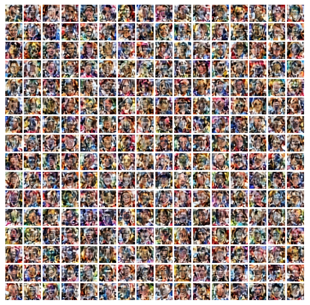
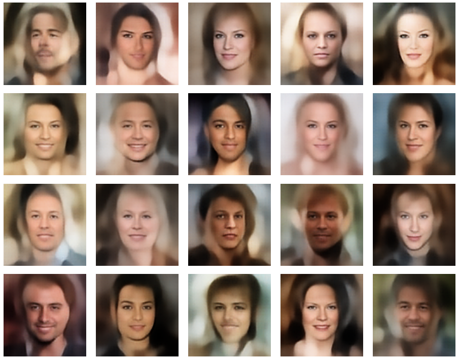
For the concrete problem of human face generation via a trained convolutional Autoencoder [CAE] I have actually found that the data produced in the CAE’s latent space can very well be described by a MND. See the posts on Autoencoders in this blog. This alone is motivation enough to dive a bit deeper into the (beautiful) mathematical properties of MNDs.
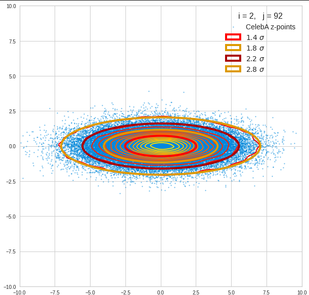
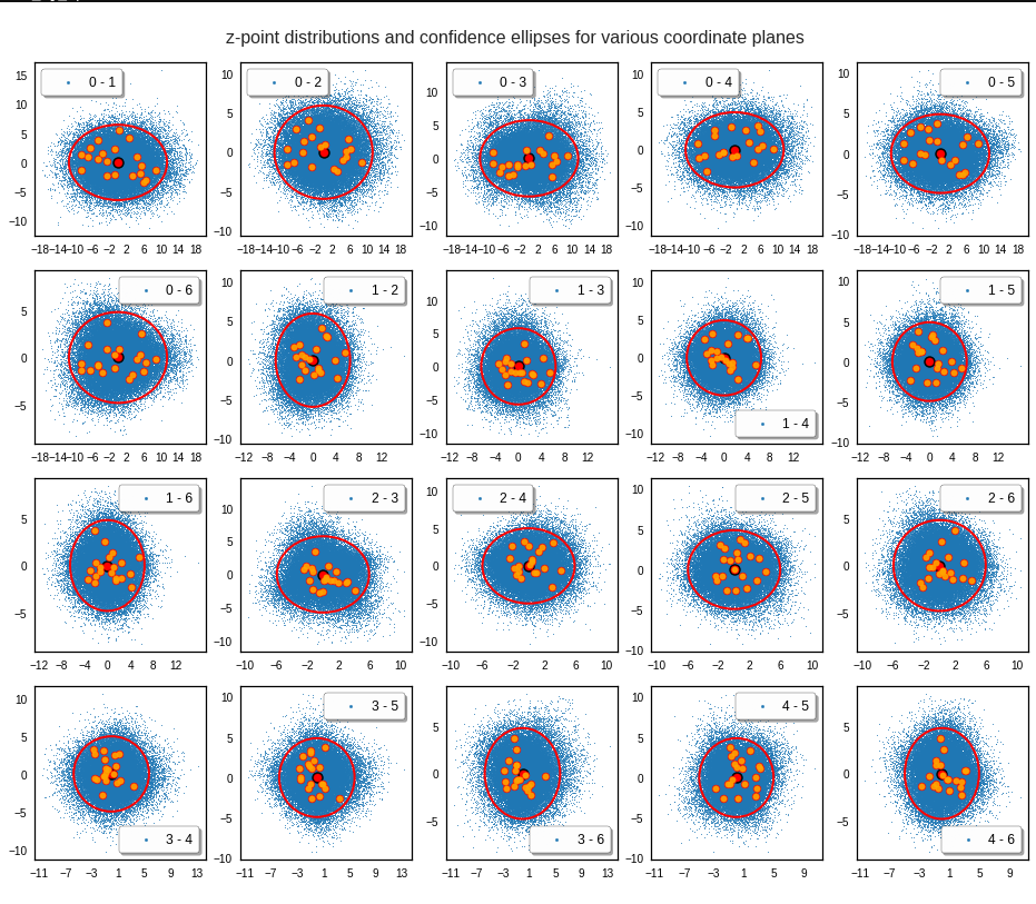
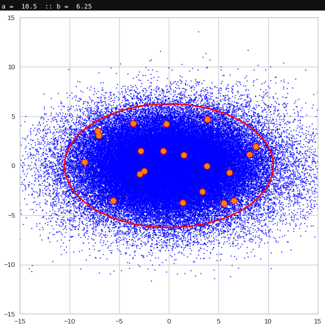
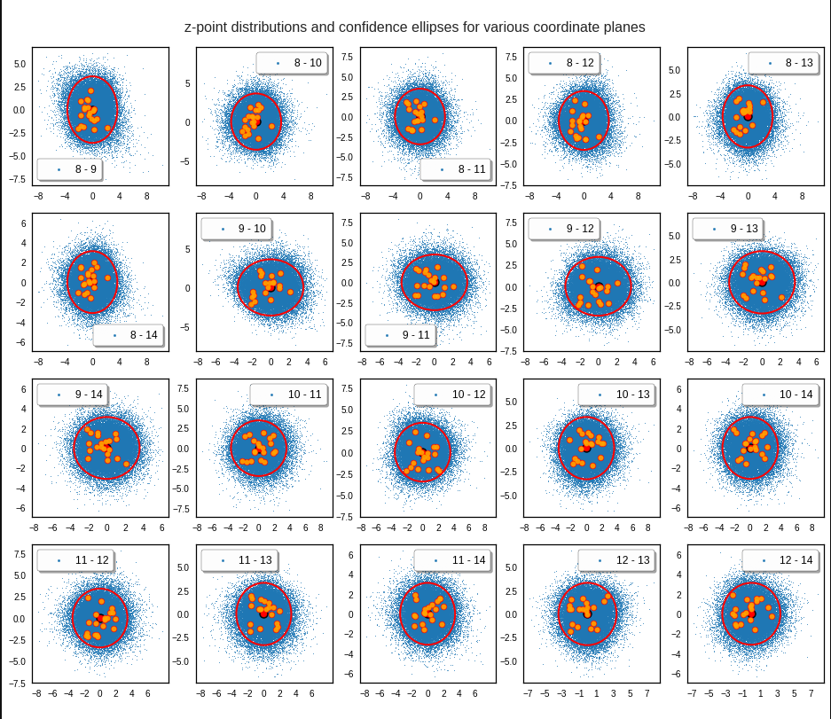
Just to illustrate it: The following plots show projections of the approximate MND onto coordinate planes.
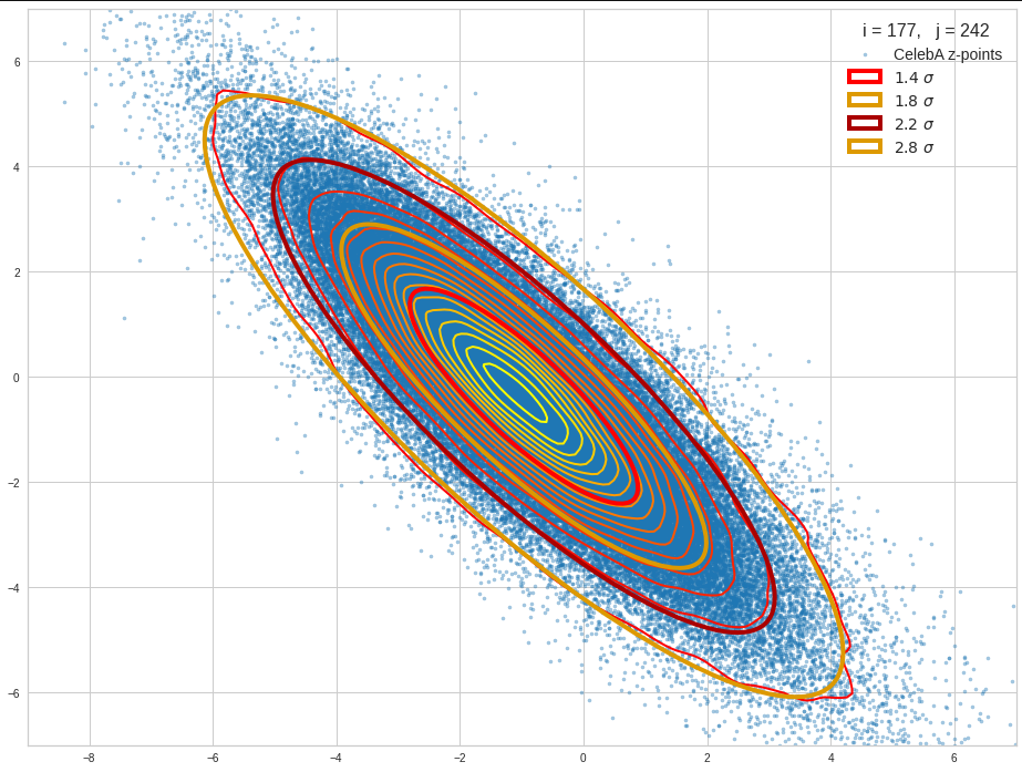
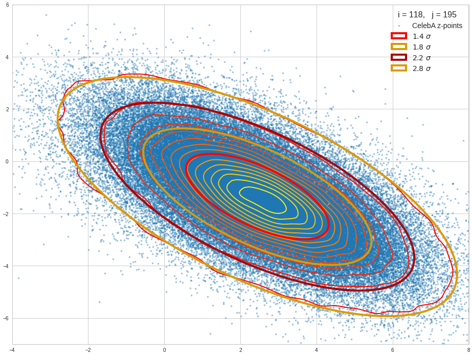
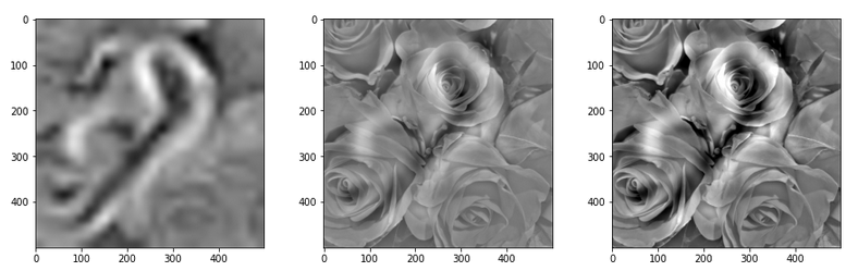
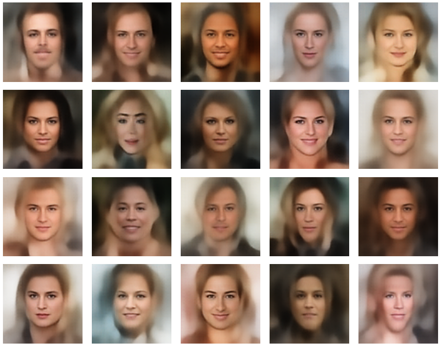
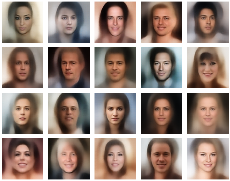
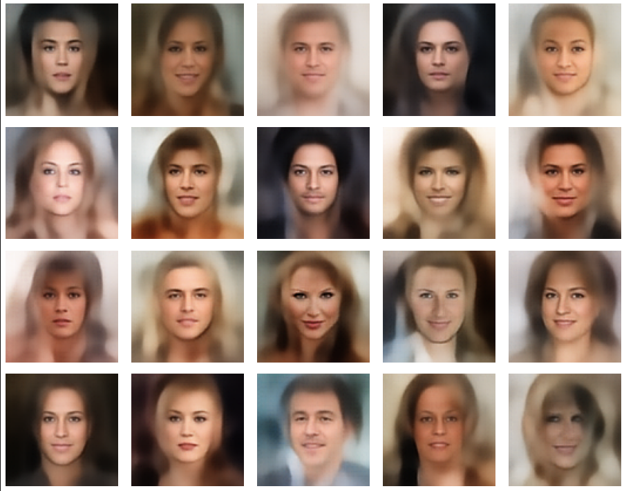
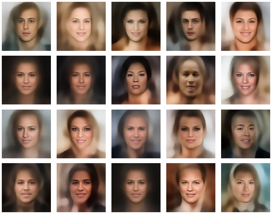
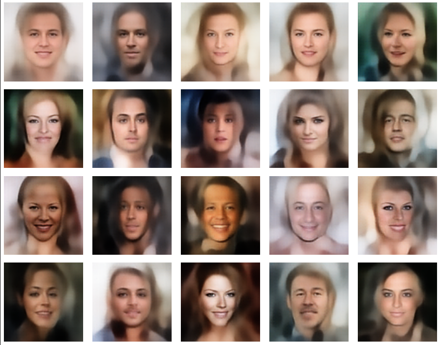
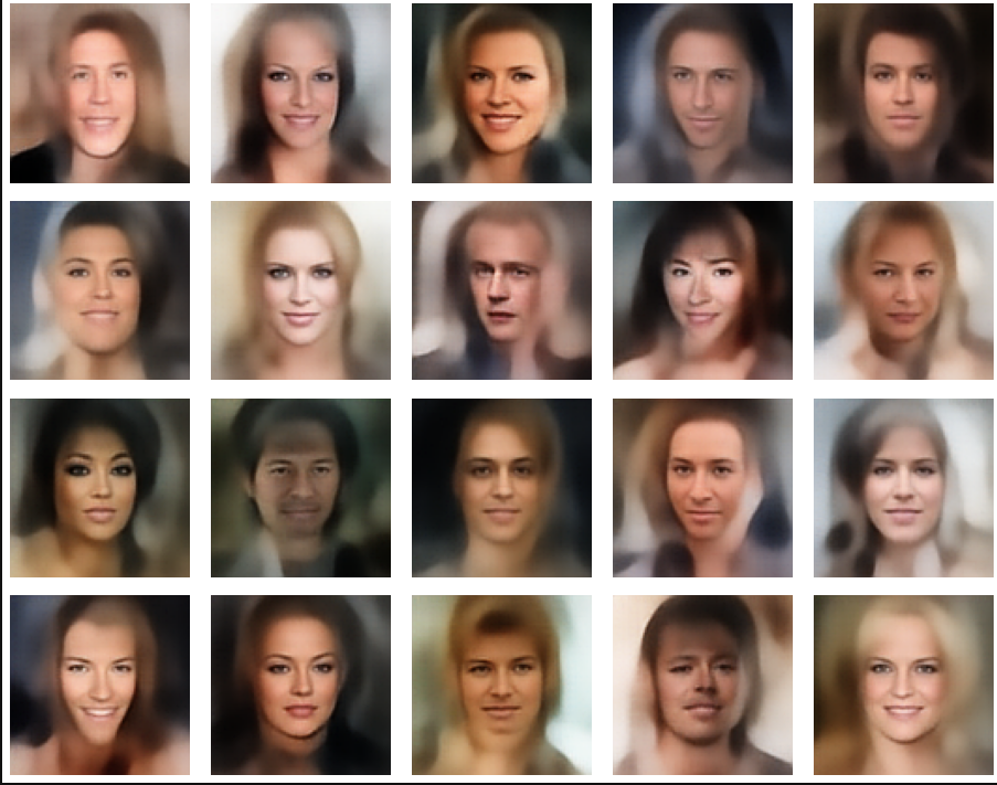
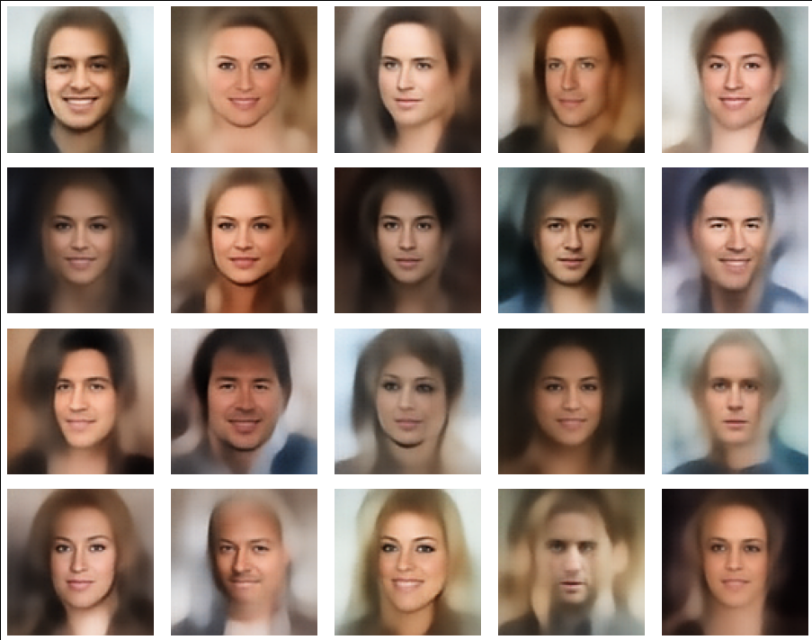
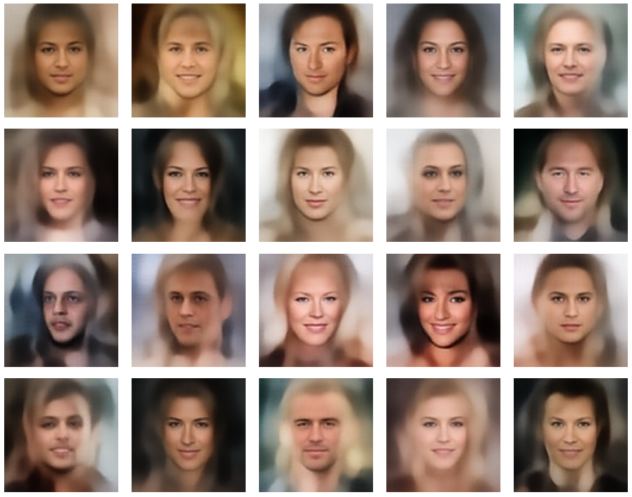
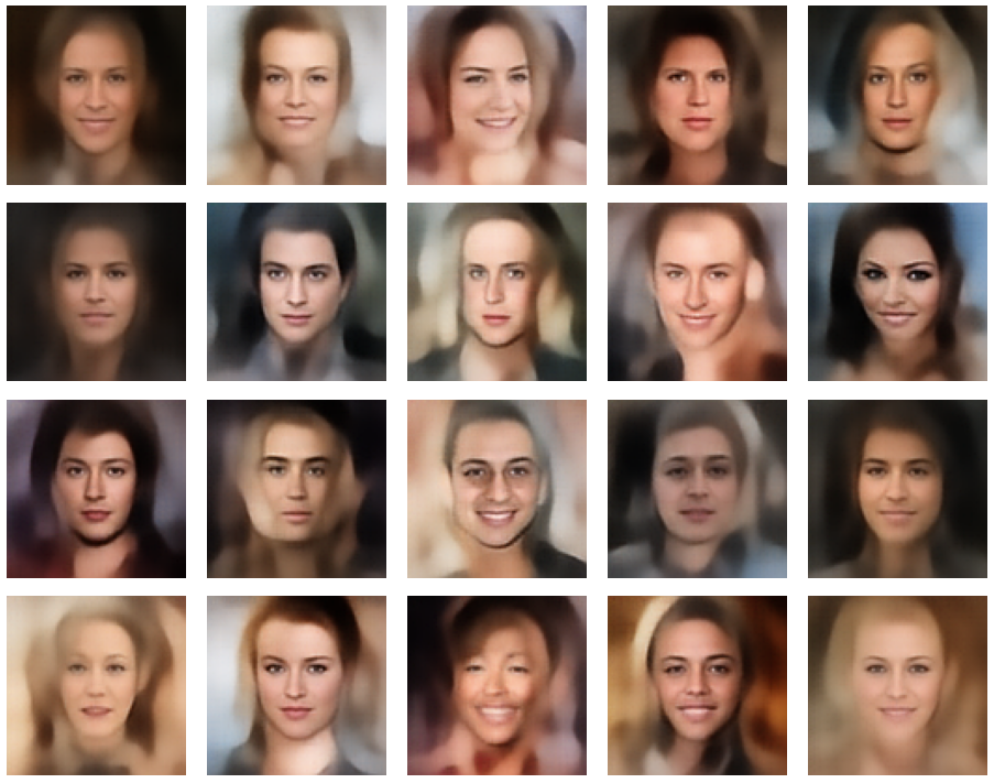
We find the typical elliptic contour lines which are to be expected for a MND. And here are some generated face images from statistical vectors which I derived from an analysis of the characteristic features of the 2-dim projections of the latent MND which my CAE had produced:
ML is math in the end – and MNDs are no exception
Some of my readers may have noticed that I wanted to start a series on the topic of creating random vectors for a given MND-like vector distribution. The characteristic parameters for the n-dimensional MND can either stem from an analysis of experimental ML data or come from theoretical sources. This was in April. But, I have been silent on this topic for a while.
The reason was that I got caught up in the study of the math of MNDs, of their properties, their marginal distributions and of quadratic forms in multiple dimensions (ellipsoids and ellipses). I had to re-collect a lot of mathematical information which I once (45 years ago) had learned at university. Unfortunately, multivariate analysis (i.e. data analysis in multidimensional spaces) requires some (undergraduate) university math. Regarding MNDs, knowledge both in linear algebra, statistics and vector analysis is required. In particular matrices, their decomposition and their geometrical interpretation play a major role. And when you try to understand a particular problem which obviously is characterized by an overlap of multiple mathematical disciplines the amount of information can quickly grow – without the connections and consistency becoming clear at first sight.
This is in part due to the different fields the authors of papers on MNDs work in and the different focuses they have on properties of MNDs. Although many introductory information about MNDs is available on the Internet, I have so far missed a coherent and comprehensive presentation which illustrates the theoretical insights by both ideal and real world examples. Too often the texts are restricted to pure formal derivations. And none of the texts discussed the problem of vector generation within the limits of MND confidence levels. But this task can become important in generative ML: At high confidence levels outliers become a strong weight – and deviations from an ideal MND may cause disturbances.
One problem with appropriate vector generation for creative ML purposes is that ML experiments deliver (latent) data which are difficult to analyze as they reside in high-dimensional spaces. Even if we already knew that they form a MND in some parts of a latent space we would have to perform a drill down to analytic formulas which describe limiting conditions for the components of the statistical vectors we want to create.
The other problem is that we need a solid understanding of confidence levels for a multidimensional distribution of data points, which we approximate by a MND. And on one’s way to understanding related properties of MNDs you pass a lot of interesting side aspects – e.g. degenerate distributions, matrix decompositions, affine transformations and projections of multidimensional hypersurfaces onto coordinate planes. Far too interesting to refrain from not writing something about it …
After having read many publicly available articles on MNDs and related math I had collected a bunch of notes, formulas and numerical experiments. The idea of a general post series on MNDs grew in parallel. From my own experiences I thought that ML people who are confronted with latent representations of data and find indications of a MND would like to have an introduction which covers the most relevant aspects of MNDs. On a certain mathematical level, and supported by illustrations from a concrete example.
But I will not forget about my original objective, namely the generation of random vectors within confidence levels. In the end we will find two possible approaches: One is based on a particular linear transformation, whose mathematical form is determined by a covariance analysis of our data distribution, and random number generators for multiple Gaussian distributions. The other solution is based on a derivation of precise conditions on random vector components from ellipses which are produced by projections of our real experimental data distribution onto coordinate planes. Such limiting conditions can be given in form of analytic expressions.
The second approach can also be understood as a reconstruction of a multivariate distribution from low-dimensional projection data:
We create vectors of a concrete MND-like vector distribution in n dimensions by only referring to characteristic data of its two-dimensional projections onto coordinate planes.
This is an interesting objective in itself as the access to and the analysis of 2-dimensional (correlated) data may be a much easier endeavour than analyzing the full distribution. But such an approach has to be supported by mathematical arguments.
Objectives of this post series
Objectives of this post series are:
- We want to find out what a MND is in mathematical and statistical terms and how it can be based on a simpler vector distributions within the ℝn.
- We want to study the basic role of a standardized multivariate normal distribution in the game and the impact of linear affine transformations on such a distribution – in terms of linear algebra and from a geometrical point of view.
- We also want to describe and interpret the difference between normal MNDs and so called degenerate MNDs.
- We want to understand the most important mathematical properties of MNDs. In particular we want to better grasp the mathematical meaning of correlations between the vector components and their impact on the probability density function. Furthermore the relation of a MND to its marginal distributions in sub-spaces of lower dimensions is of major interest.
- We want to formally create a MND-approximation to a real multivariate data distribution by an analysis of real distribution’s properties and in particular from parameters describing the correlations between the vector components. Of particular interest are the covariance matrix and the precision or correlation matrix.
- We want to study the role of projections when turning from a MND to its marginal distributions and the impact of such projections on the matrices qualifying the original and its marginal distributions.
- We want to understand the form of contour hyper-surfaces for constant probability density values of a MND. We also want to derive what the projections of these hyper-surfaces onto coordinate planes look like.
- We want to show that both contour hyper-surfaces of the MND and of its projections in marginal distributions contain the same proportions of integrated data points and, equivalently, the same probability proportions resulting from an integration of the probability density from the distribution’s center up to the hyper-surfaces.
- We want to illustrate basic MND-creation principles and the effects of linear affine transformations during the construction process by an ideal 3-dimensional MND example and by projections of a real vector distribution from an ML-experiment onto 2-dimensional and 3-dimensional sub-spaces. We also want to illustrate the relation between the MND and its marginal distributions by plotting concrete 3-dimensional examples and their projections onto coordinate planes.
- We want to use the derived MND properties for the creation of statistical vectors v which fulfill the following conditions:
- Each of the generated v is a member of a vector population, which has been derived from a ML experiment and which to a good approximation can be described by a MND (and its extracted basic parameters).
- Each v has an endpoint within the multidimensional volume enclosed by a contour-hypersurface of the MND’s probability density function [p.d.f.],
- The limiting hypersurface is defined by a chosen confidence level.
- We want to create statistical vectors within the limit of contour hyper-surfaces by using elementary construction principles of a MND.
- In a second approach we want to reduce vector creation to solving a sequence of 2-dimensional problems. I.e. we want to work with 2-dim marginal distributions in 2-dim sub-spaces of the ℝn. We hope that the probability density functions of the relevant distributions can be described analytically and provide computable limiting conditions on vector components.
Note: The production of statistical vectors from data of projected low-dimensional marginal distributions corresponds to a reconstruction of the full MND from its projections. - During random vector creation we want to avoid PCA-transformations of the whole real data distribution or of projections of it.
- Based on MND-parameters we want to find analytic expressions for the vector component limits whenever possible.
The attentive reader has noticed that the list above includes an assumption – namely that a multidimensional contour hypersurface of a MND can be associated with something like a confidence level. In addition we have to justify mathematically that the reduction to data of 2-dimensional projections of the full vector distribution is a real option for statistical vector creation.
The last three points are a bit tough: Even if we believe in math textbooks and get limiting hyper-curves of a quadratic form in our coordinate planes the main axes of the respective ellipses may show angles versus the coordinate axes (see the example images above). All this would have to be taken care of in a precise analytic form of the limits which we impose on the components of our aspired statistical vectors.
So, this series is, at least in parts, going to be a tough, but also very satisfactory journey. Eventually, after having clarified diverse properties of MNDs and their marginal distributions in lower dimensional spaces, we will end up with quadratic equations and some simple matrix operations.
Objectives of the next post
We must not forget that statistics plays a major role in our business. In ML we deal with finite collections (samples) of individual object data which are statistically picked from a greater population (with assumed statistical properties). An example is a concrete collection of images of human faces and/or their latent vectors. The data can be organized in form of a two-dimensional data matrix: Its rows may indicate individual objects and its columns properties of these objects (or vice versa). In either direction we have vectors which focus on a particular aspect of the data: Individual objects or the statistics of a specific object property.
While we are used to univariate “random variables” we have to turn to so called “random vectors” to describe multidimensional statistical distributions and respective samples picked from an underlying population. A proper vector notation will give us the advantage of writing down linear transformations of a whole multidimensional vector distribution in a short and concise form.
Besides introducing random vectors and their components the next post
Multivariate Normal Distributions – II – random vectors and their covariance matrix
will also discuss related probability densities, expectation values and the definition of a covariance matrix for a random vector. Some simple properties of the covariance matrix will help us in further posts.