Statistical vector generation for multivariate normal distributions – I – multivariate and bi-variate normal distributions from CAEs

Posted on 6. July 2023 by eremo

Convolutional Autoencoders and multivariate normal distributions

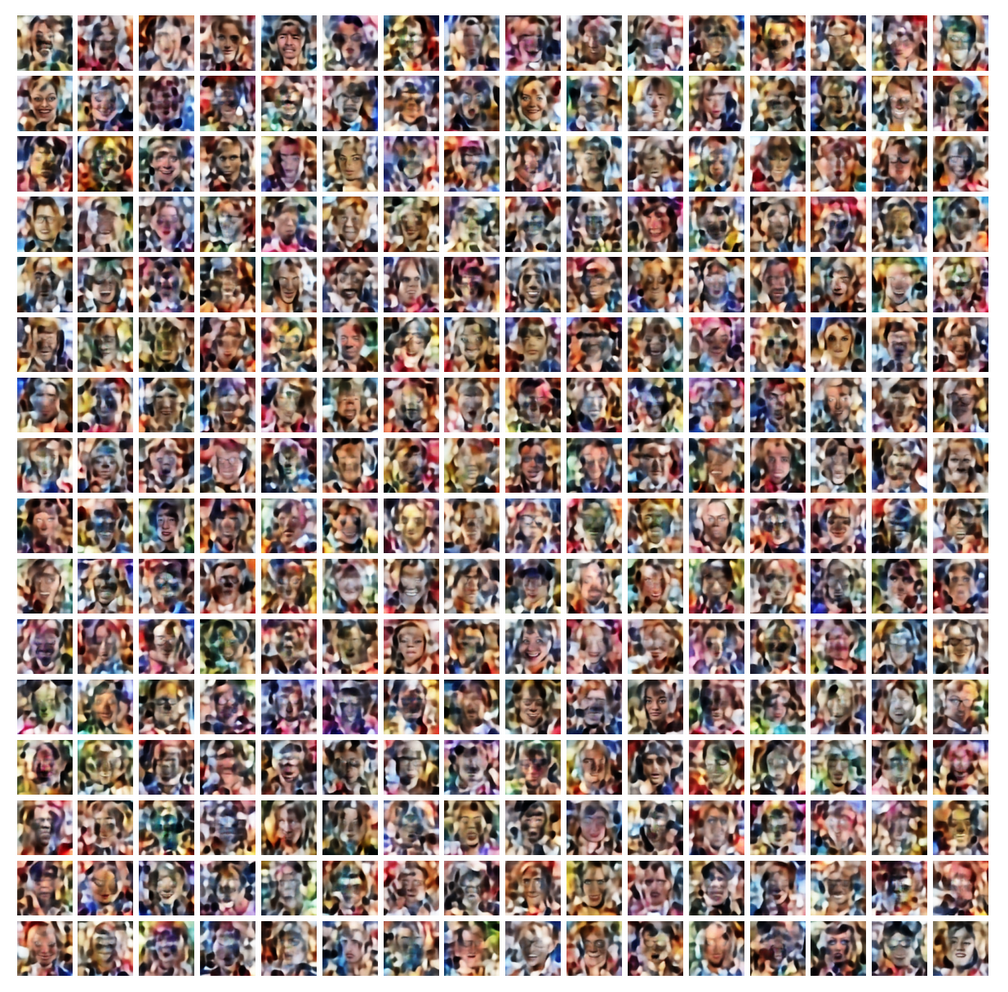
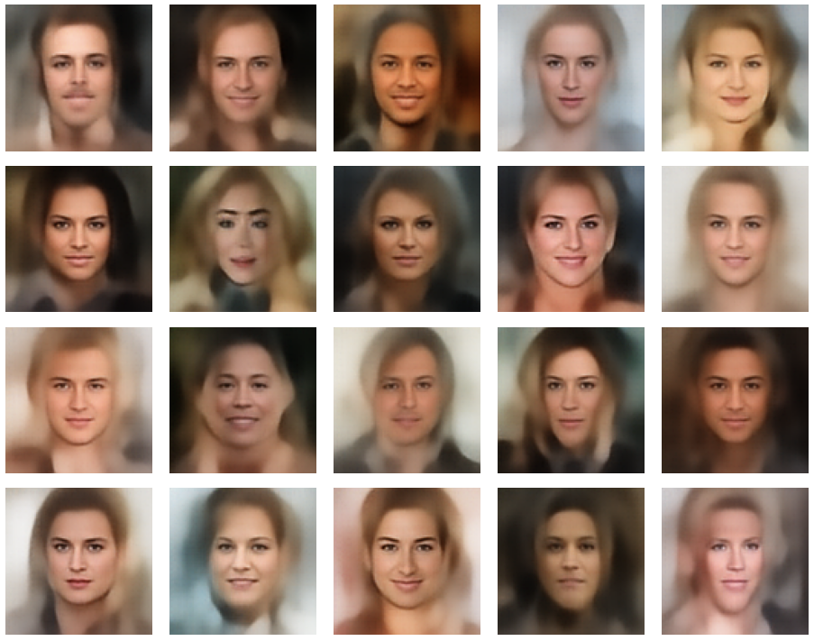
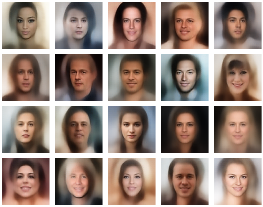
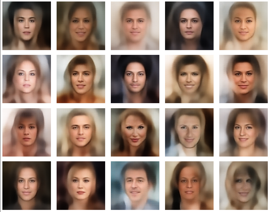
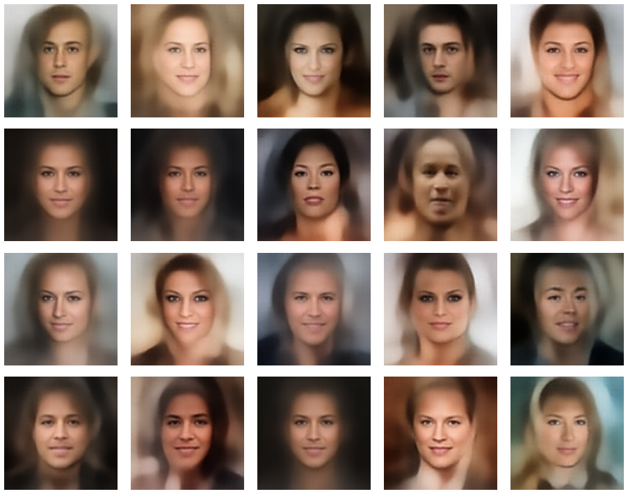
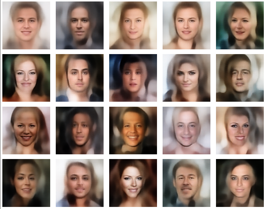
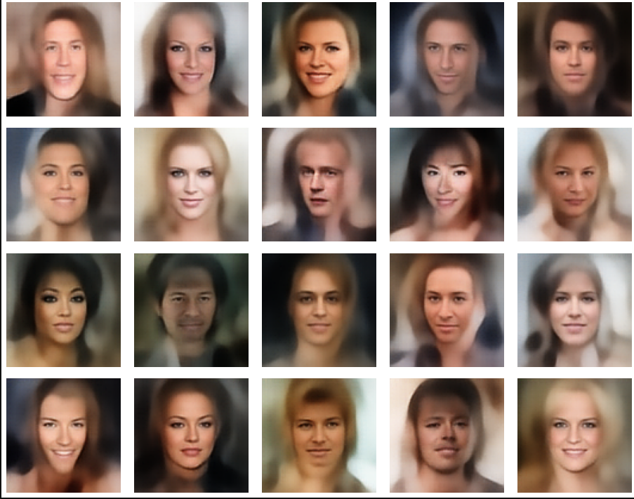
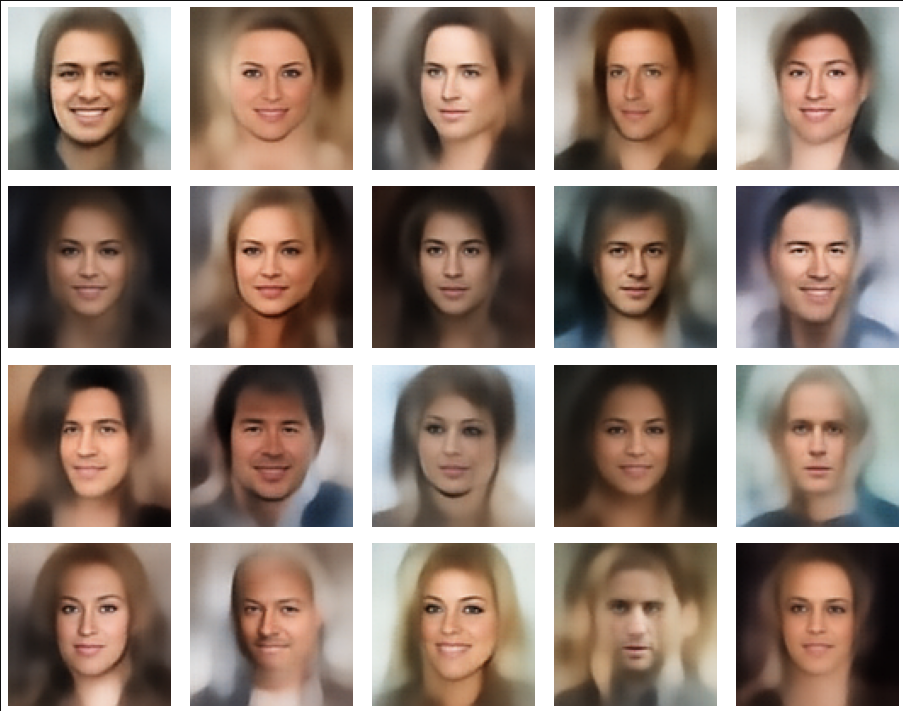
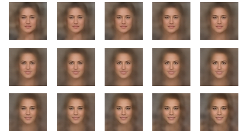
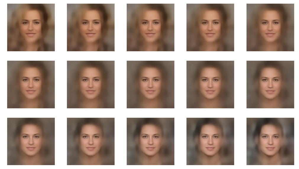
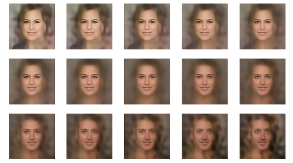
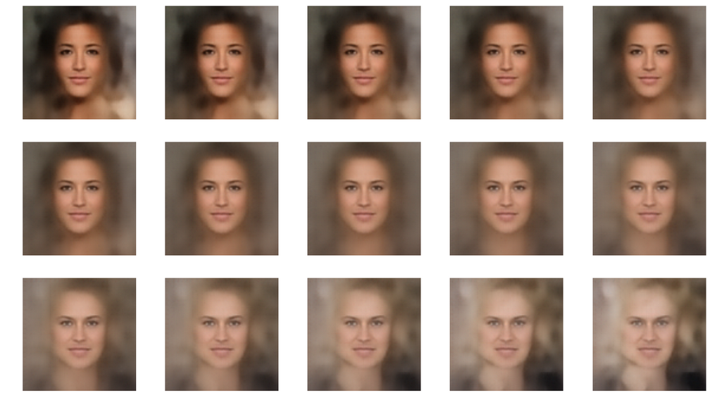
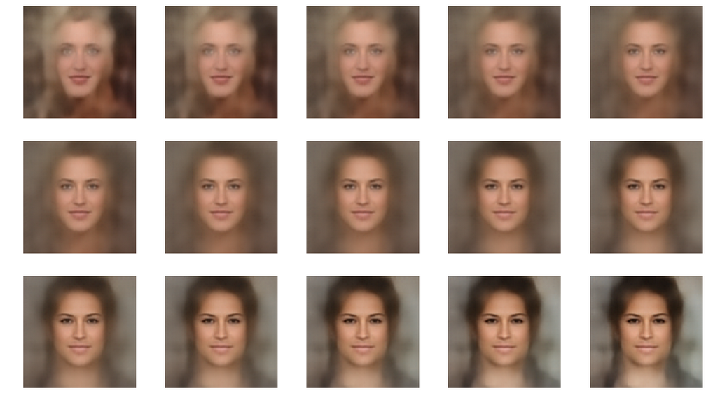
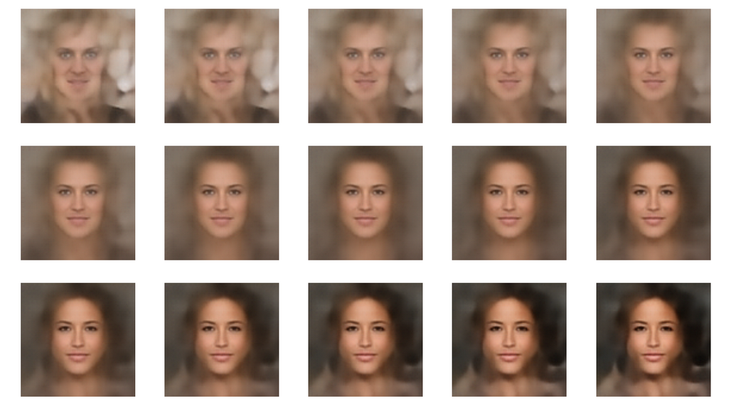
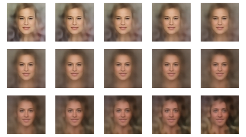
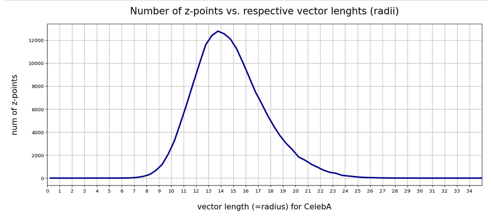
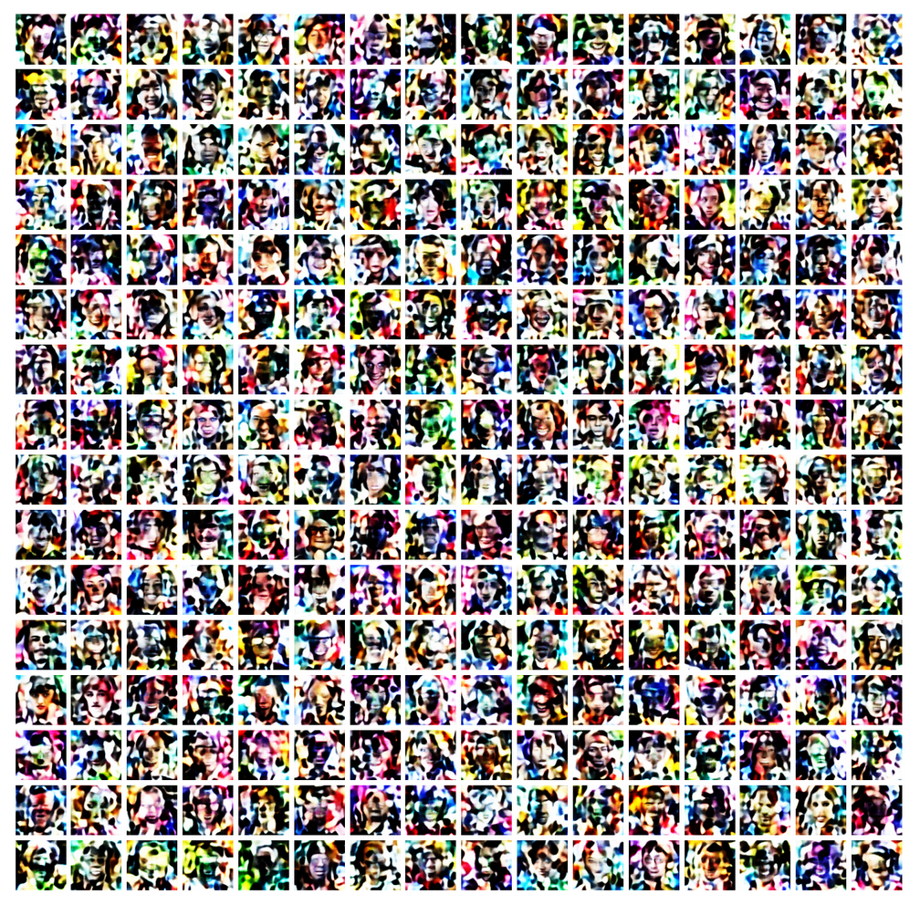
Experiments as with my own on convolutional Autoencoders [CAE] show: A CAE maps a training set of human face images (e.g. CelebA) onto an approximate multivariate vector distribution in the CAE’s latent space Z. Each image corresponds to a point (z-point) and a corresponding vector (z-vector) in the CAE’s multidimensional latent space. More precisely the results of numerical experiments showed:

The multidimensional density function which describes the inner dense core of the z-point distribution (containing more than 80% of all points) was (aside of normalization factors) equivalent to the density function of a multivariate normal distribution [MND] for the respective z-vectors in an Euclidean coordinate system.

For results of my numerical CAE-experiments see
Autoencoders and latent space fragmentation – X – a method to create suitable latent vectors for the generation of human face images
and related previous posts in this blog. After the removal of some outliers beyond a high sigma-level (≥ 3) of the original distribution the remaining core distribution fulfilled conditions of standard tests for multivariate normal distributions like the Shapiro-Wilk test or the Henze-Zirkler test.

After a normalization with an appropriate factor the continuous density functions controlling the multivariate vector distribution can be interpreted as a probability density function [p.d.f.]. The components v_j (j=1, 2,…, n) of the vectors to the z-points are regarded as logically separate, but not uncorrelated variables. For each of these variables a component specific value distribution V_j is given. All these marginal distributions contribute to a random vector distribution V, in our case with the properties of a MND:

\[ \boldsymbol{V} \: = \: \left( \, V_1, \, V_2, \, ….\, V_n\, \right) \: \sim \: \boldsymbol{\mathcal{N_n}} \, \left( \, \boldsymbol{\mu} , \, \boldsymbol{\Sigma} \, \right), \\ \quad \mbox{with} \: \boldsymbol{\mathcal{N_n}} \: \mbox{symbolizing a MND in an n-dimensional space}
\]

μ is a vector with all mean values μ_j of the V_j component distributions as its components. Σ abbreviates the covariance matrix relating the distributions V_j with one another.

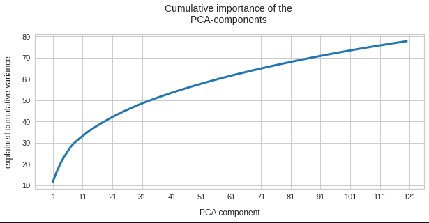
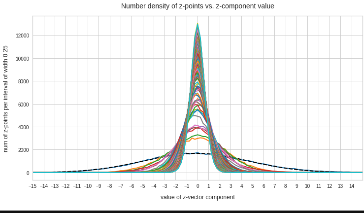
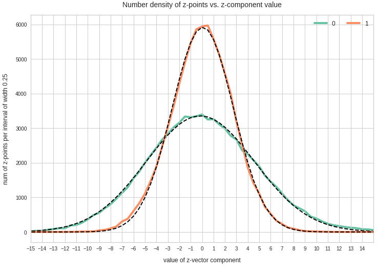
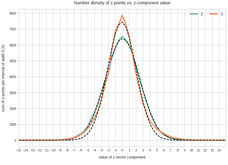
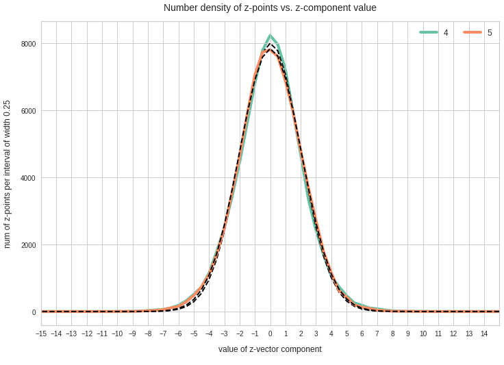
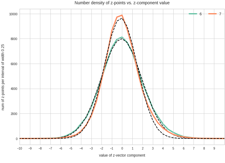
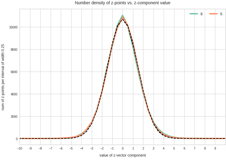
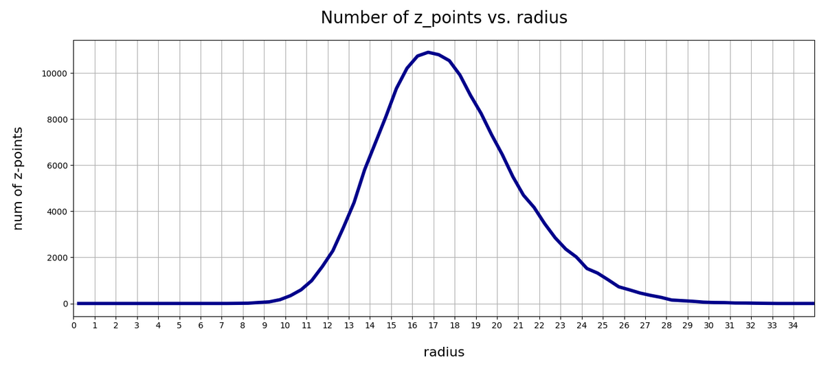
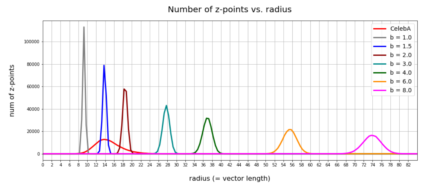
The point distribution of a CAE’s MND forms a complex rotated multidimensional ellipsoid with its center somewhere off the origin in the latent space. The latent space itself typically has many dimensions. In the case of my numerical experiments the number of dimension was n ≥ 256. The number of sample vectors used were between 80,000 and 200,000 – enough data to approximate the vector distribution by a continuous density function. The densities for the V_j-distributions formed a smooth Gaussian function (for a reasonable sampling interval). But note: One has to be careful: The fact that the V_j have a Gaussian form is not a sufficient condition for a MND. (See the next post.) But if a MND is given all V_j have a Gaussian form.

Generative use of MNDs in multidimensional latent spaces of high dimensionality

When we want to use a CAE as a generative tool we need to solve a problem: We must create statistical vectors which point into the (multidimensional) volume of our point distribution in the latent space of the encoding algorithm. Only such vectors provide useful information to the Decoder of the CAE. A full multivariate normal distribution and hyperplanes of its multidimensional density function are difficult to analyze and to control when developing a proper numerical algorithm. Therefore I want to reduce the problem of vector generation to a sequence of viewable and controllable 2-dimensional problems. How can this be achieved?

A central property of a multivariate normal distribution helps: Any sub-selection of m vector-component distributions forms a multivariate normal distribution, too (see below). For m=2 and for vector components indexed by (j,k) with respective distributions V_j, V_k we get a so called “bivariate normal distribution” [BND]:

\[ V_{jk} \: \sim \: \mathcal{N}_2\left(\, (\mu_j, \mu_k), (\,\sigma_j, \sigma_k \,) \, \right)
\]

A MND has n*(n-1)/2 such subordinate BNDs. The 2-dim density function of a bivariate normal distribution

\[ g_{jk}\,\left( \, v_j, \, v_k\, \right) \: = \: g_{jk}\,\left( \, v_j, \, v_j, \, \mu_j, \, \mu_k, \, \sigma_j, \sigma_k, \, \sigma_{jk}, … \right)
\]

for vector component values v_j, v_k defines a point density of the sample data in the (j,k)-coordinate plane of the Euclidean coordinate system in which the MND is described. The density function of the marginal distributions V_j showed the typical Gaussian forms of a univariate normal distribution.

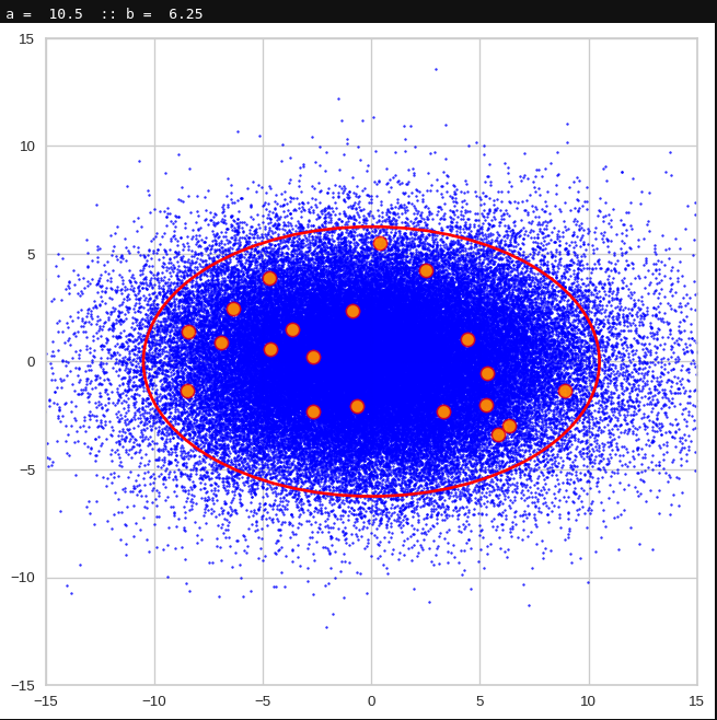
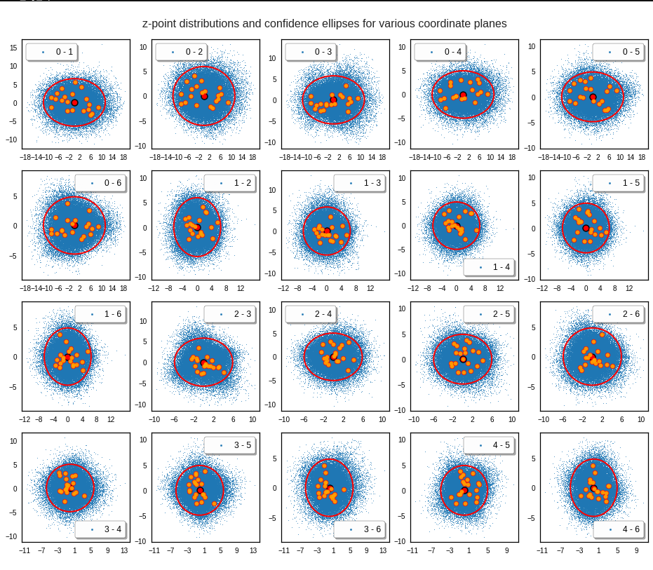
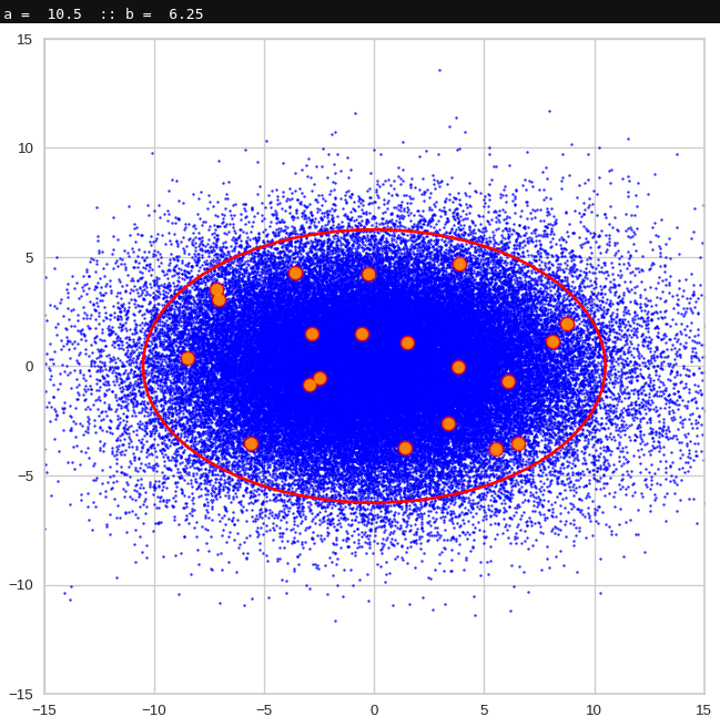
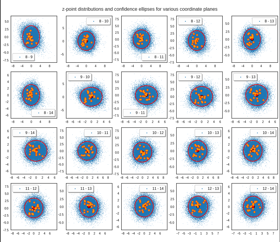
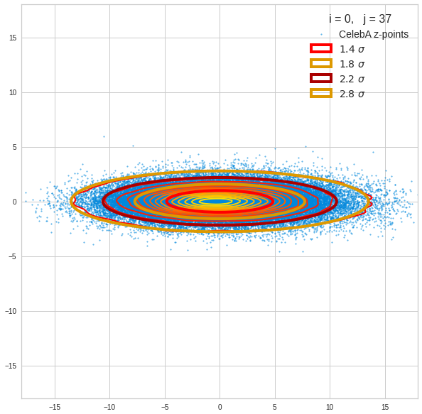
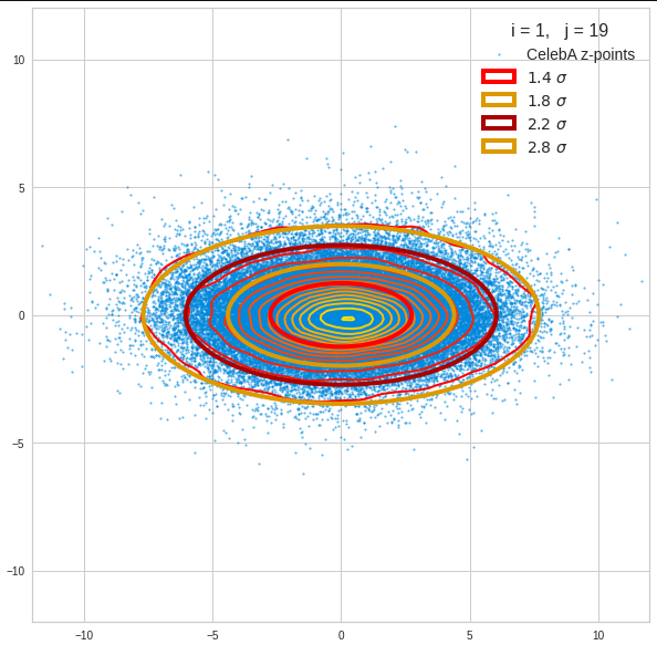
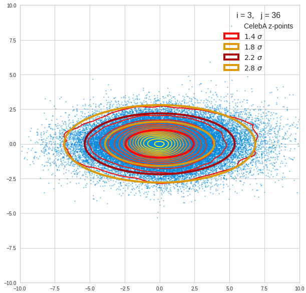
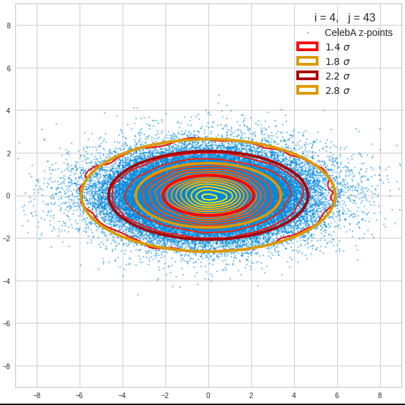
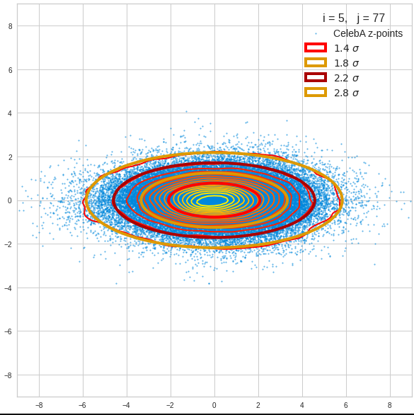
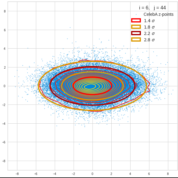
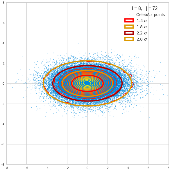
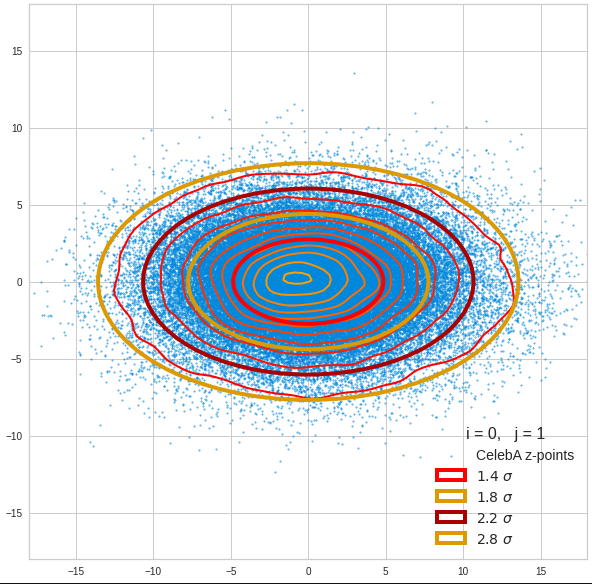
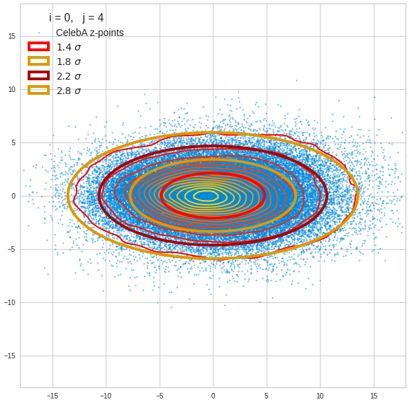
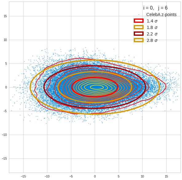
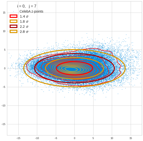
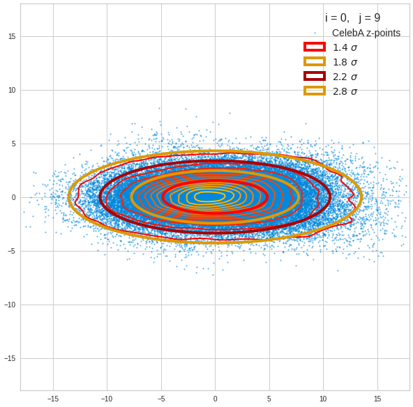
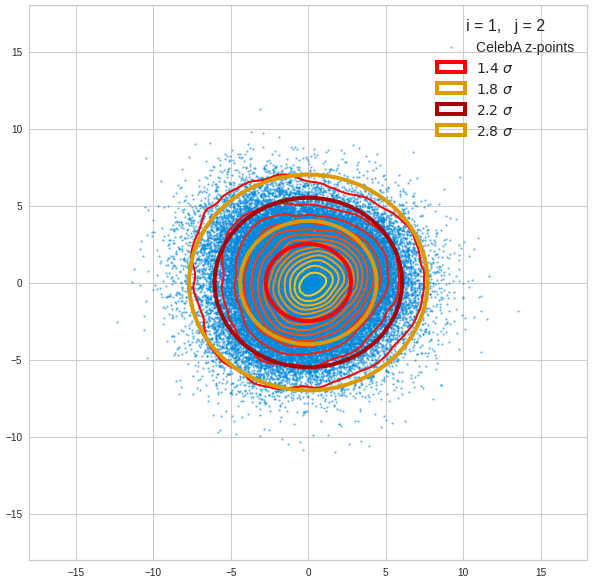
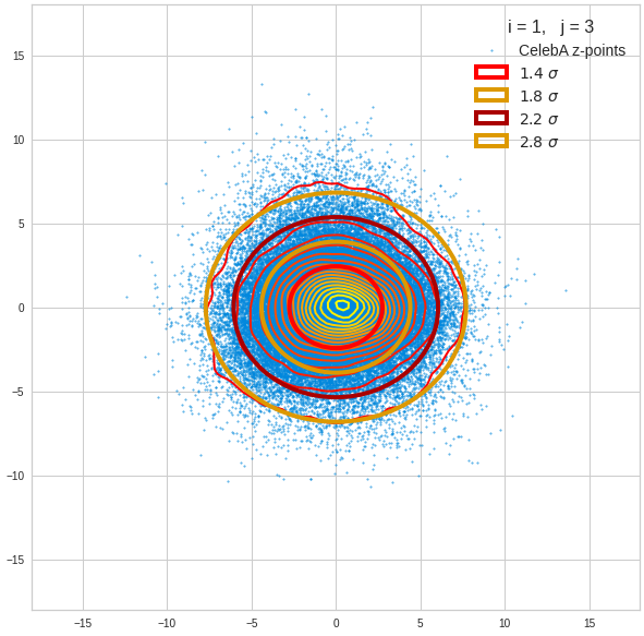
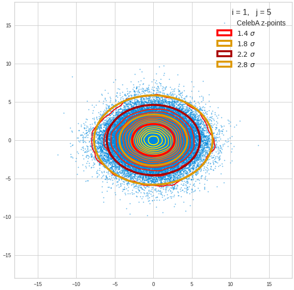
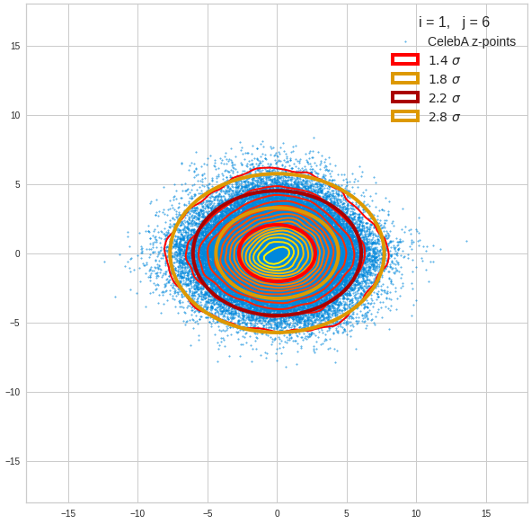
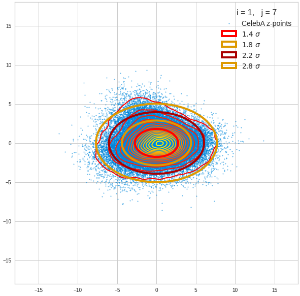
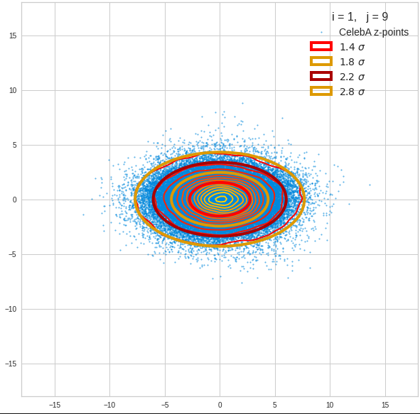
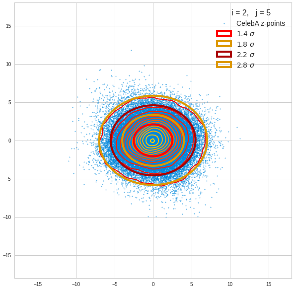
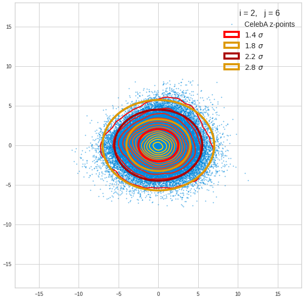
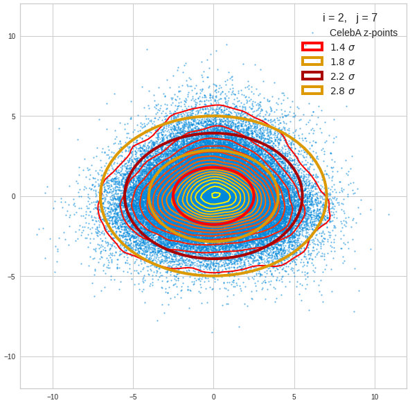
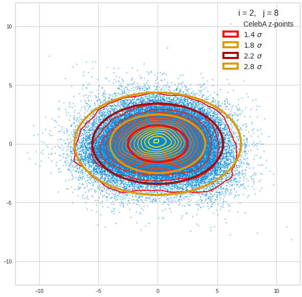
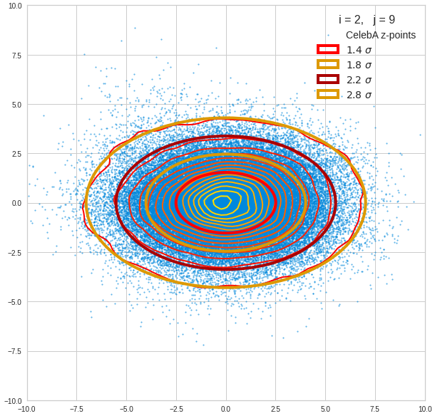
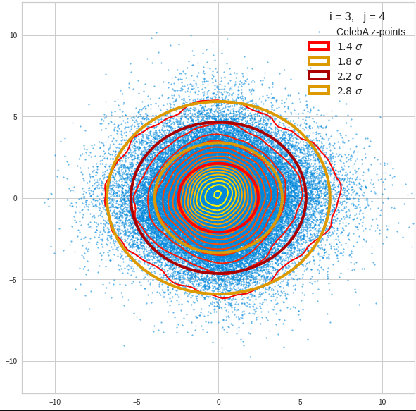
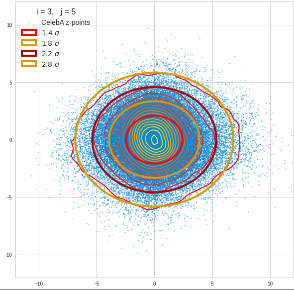
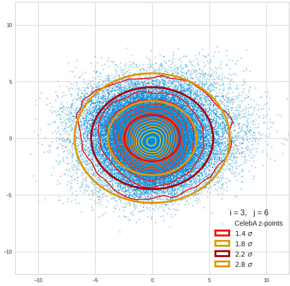
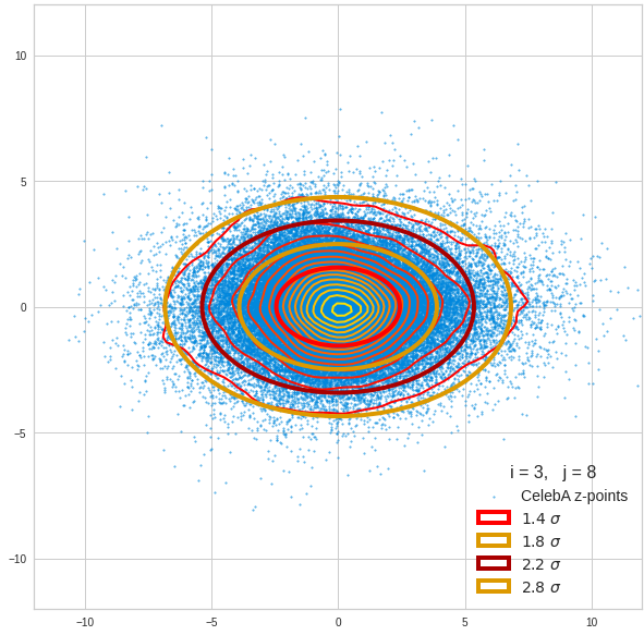
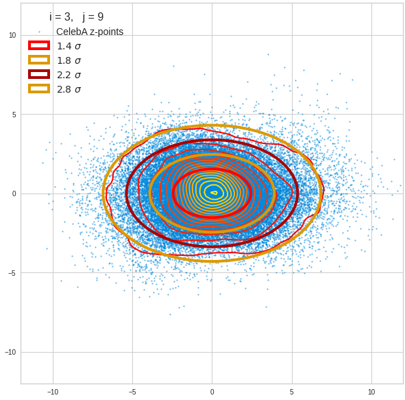
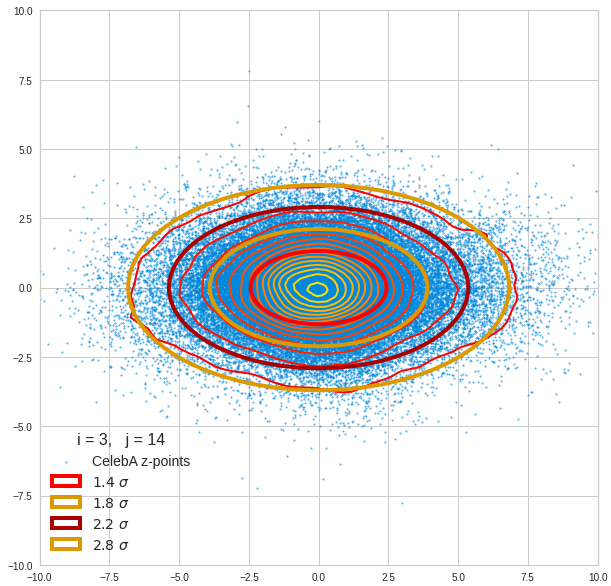
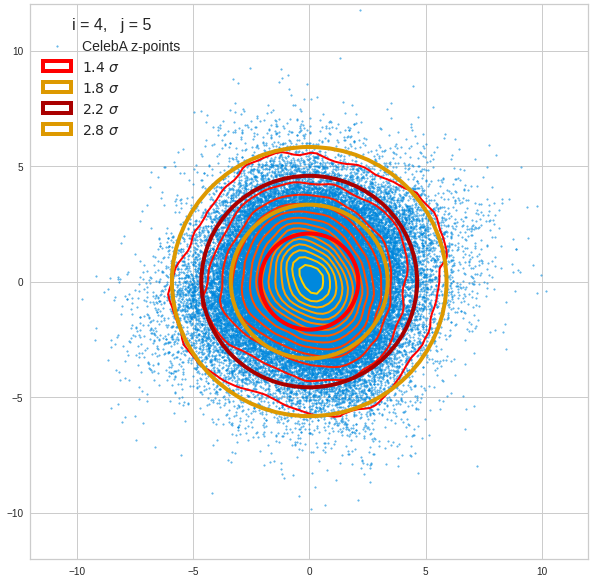
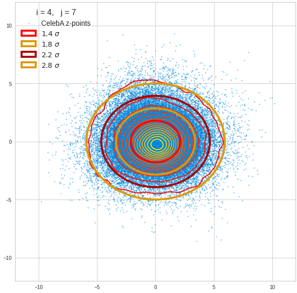
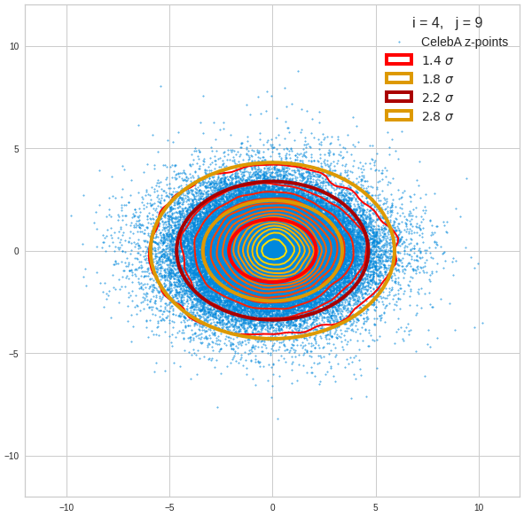
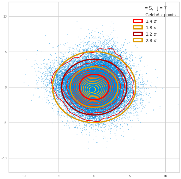
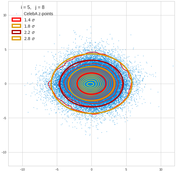
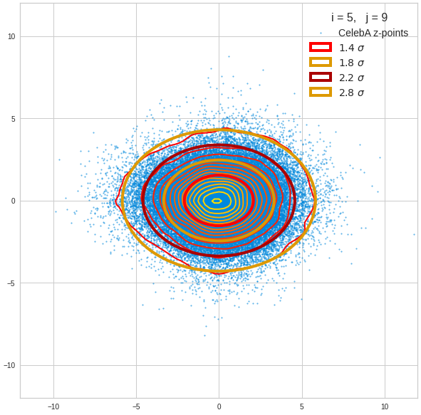
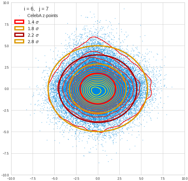
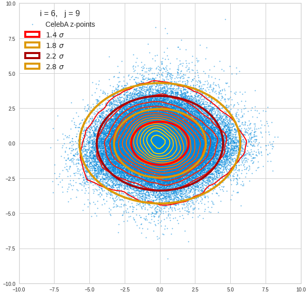
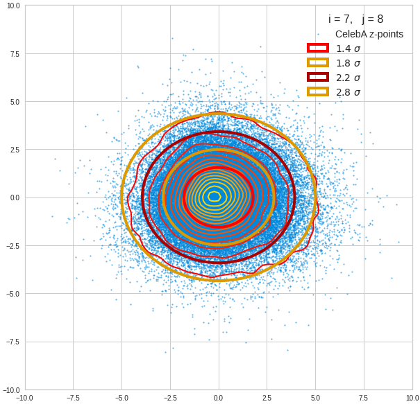
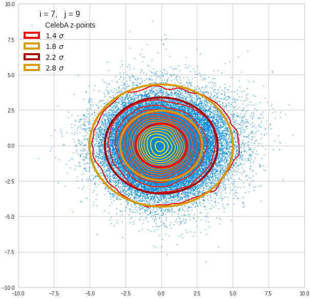
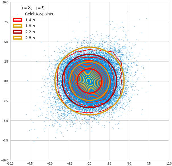
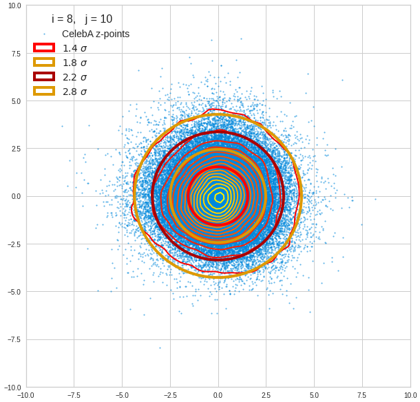
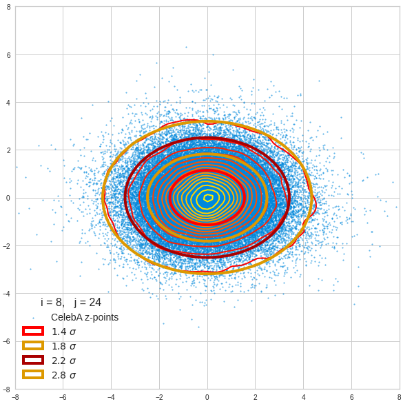
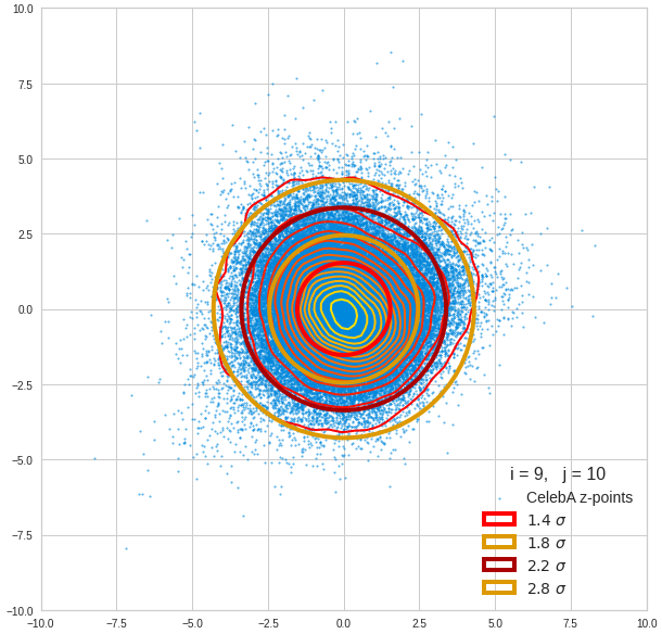
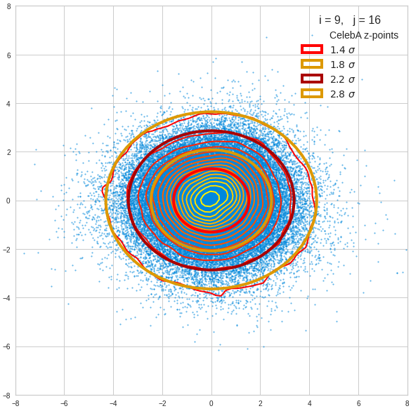
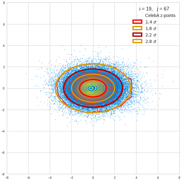
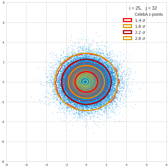
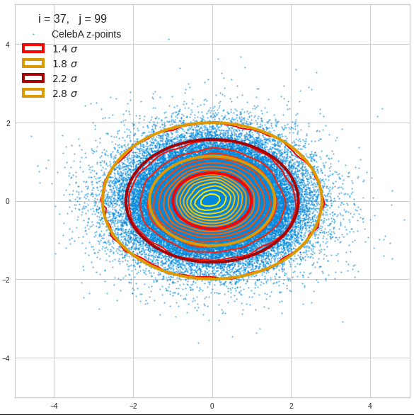
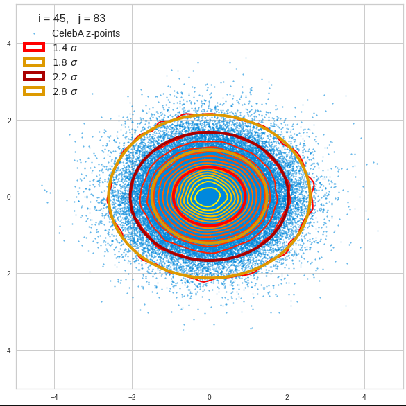
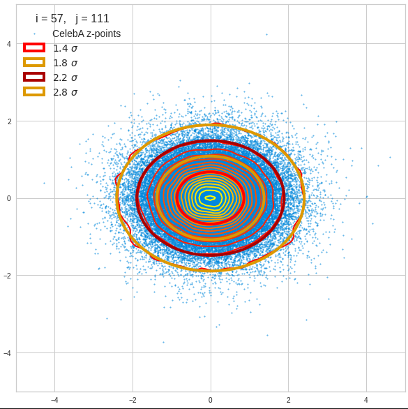
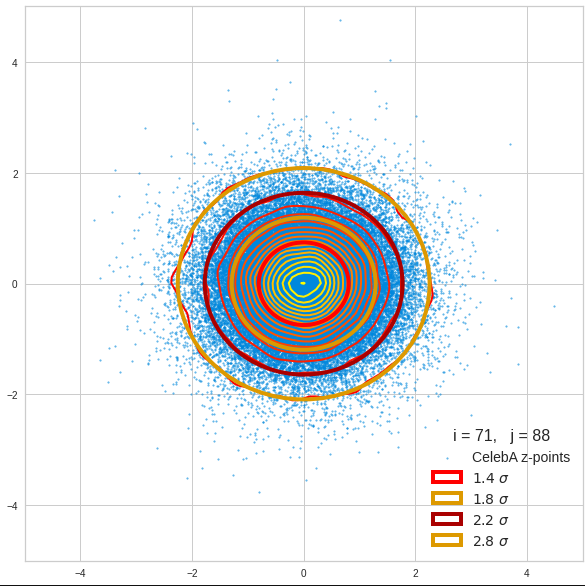
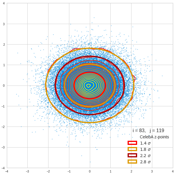
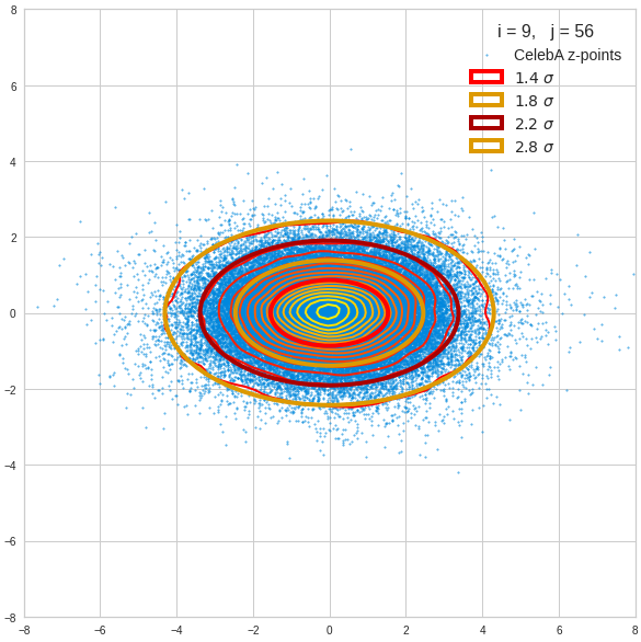
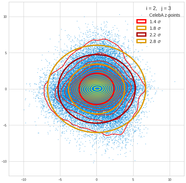
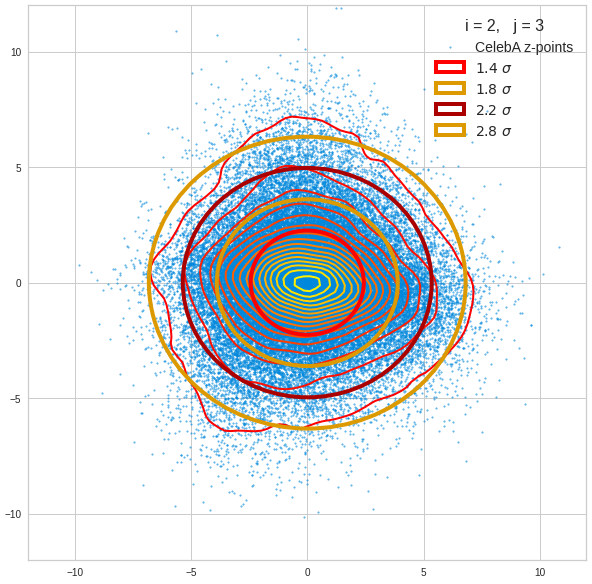
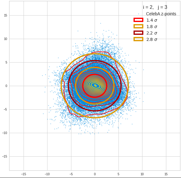
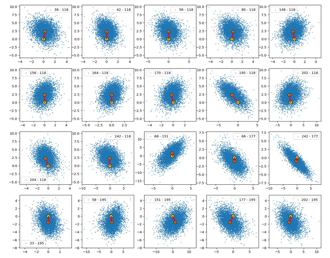
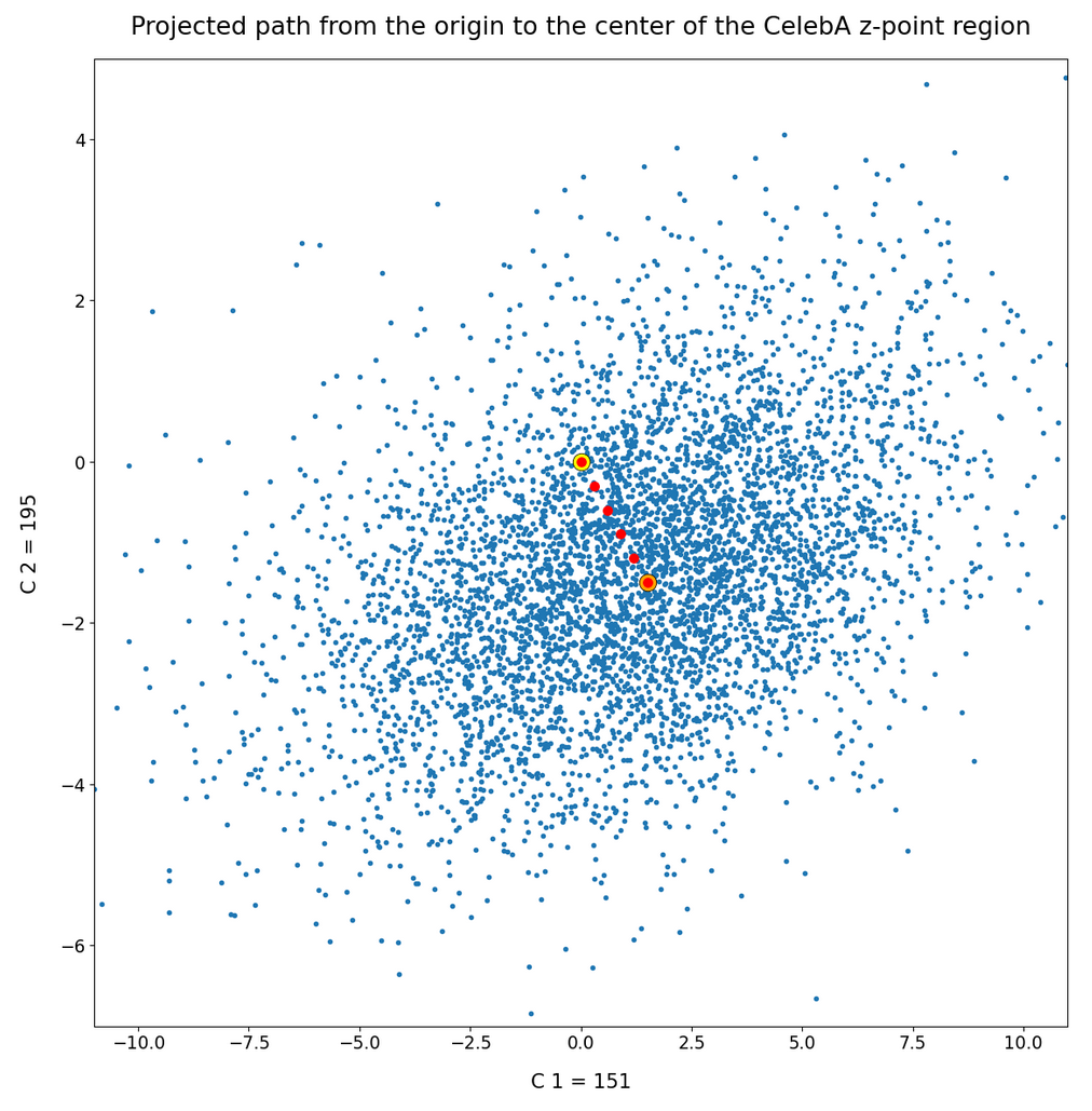
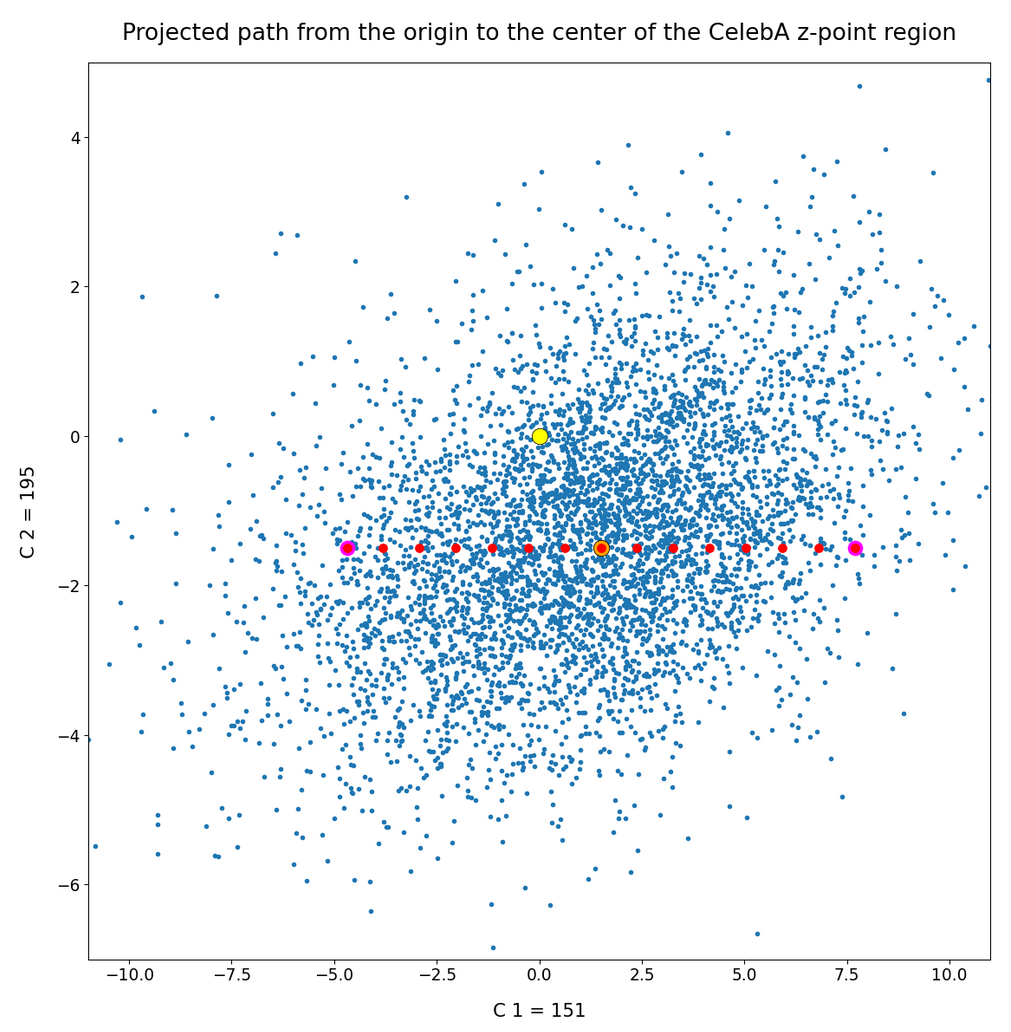
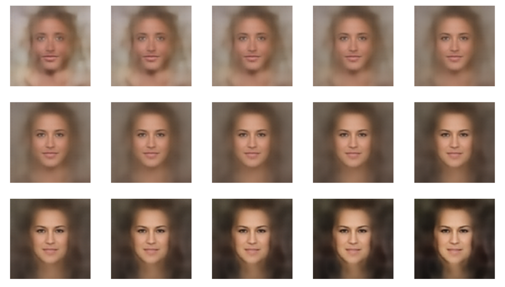
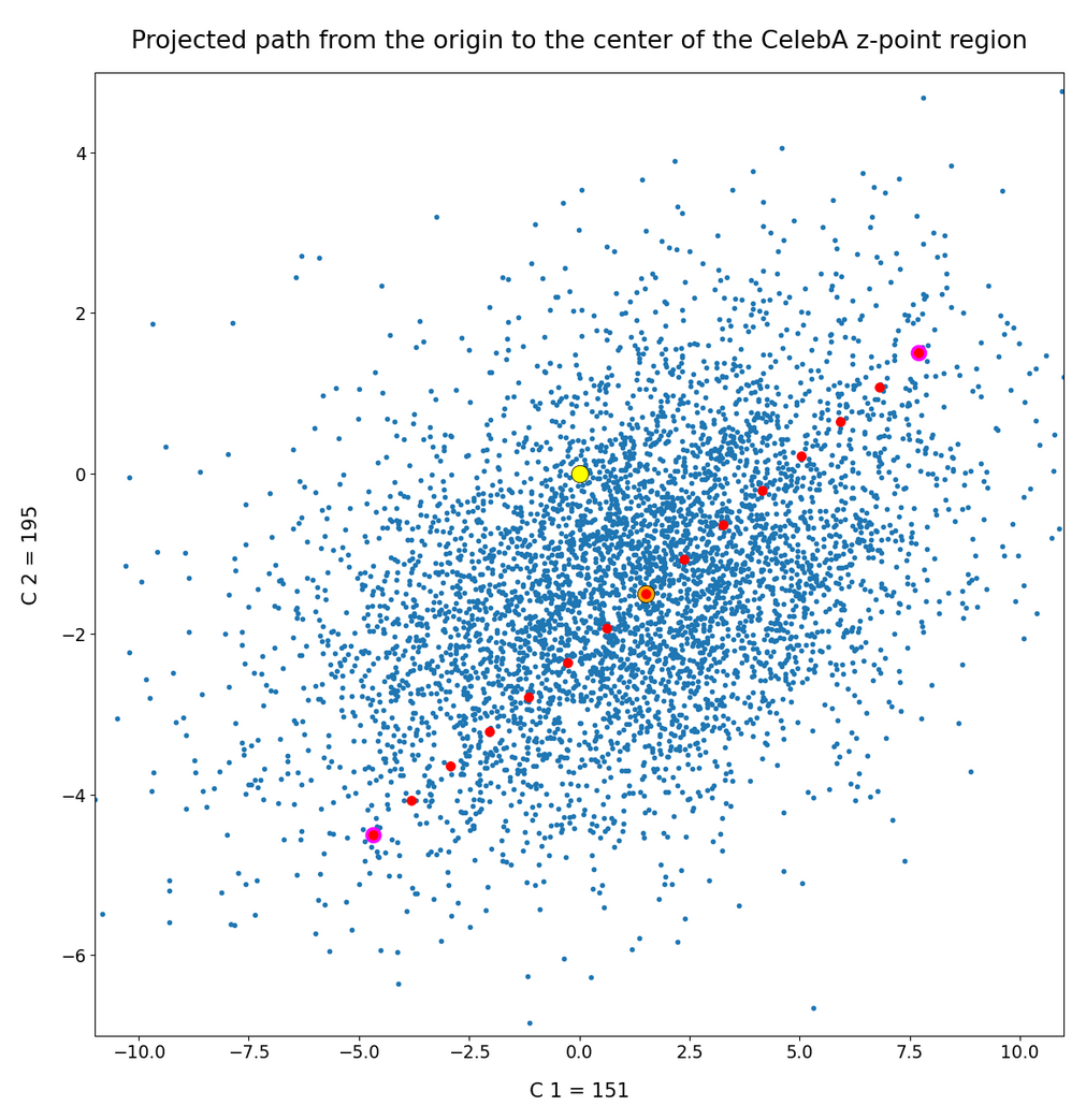
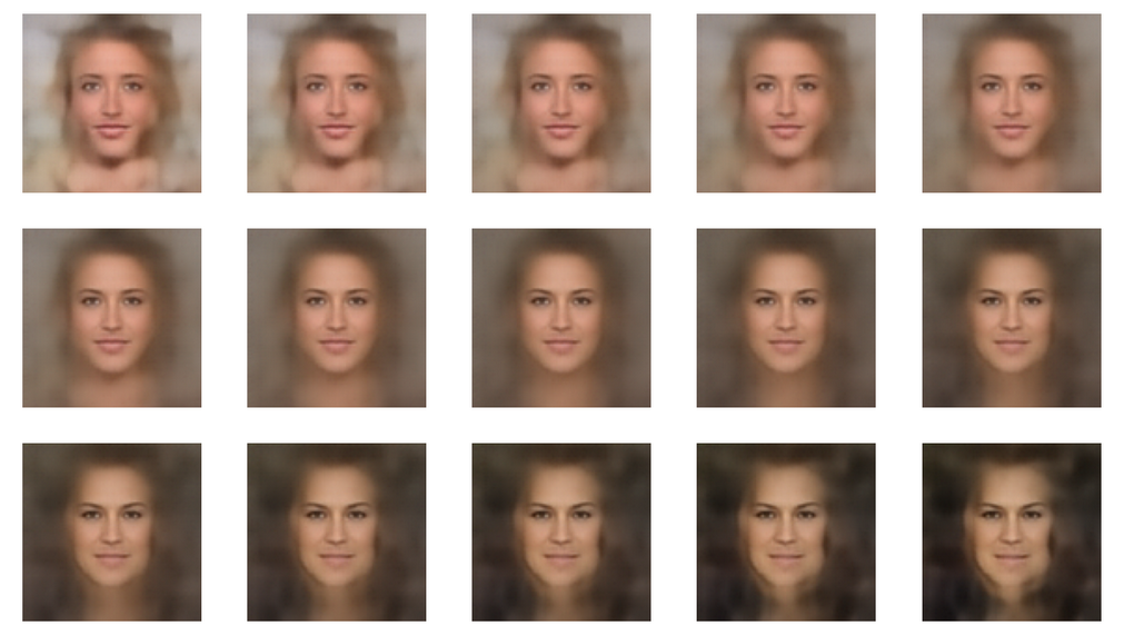
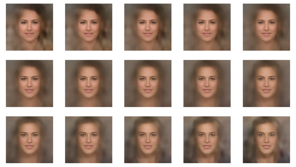
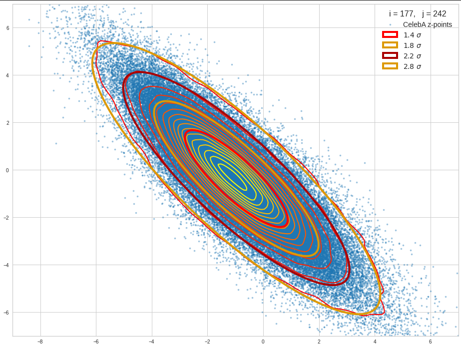
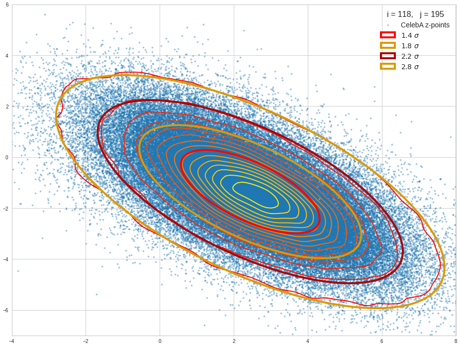
The density function of a BND has some interesting mathematical properties. Among other things: The hyperplanes of constant density of a BND’s density function form ellipses. This is illustrated by the following plots showing such contour lines for selected pairs (V_j, V_k) of a real point-distribution in a 256-dimensional latent space. The point distribution was created by a CAE in its latent space for the CelebA dataset.

Contour lines for selected (j,k)-pairs. The thick lines stem from theory and calculated correlation coefficients of the univariate distributions.

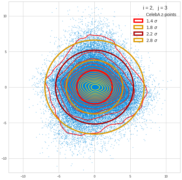
The next plot shows the contours of selected vector-component pairs after a PCA-transformation of the full MND. (Main ellipse axes are now aligned with the axes of the PCA-coordinate system):

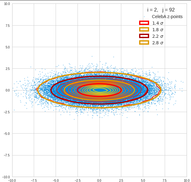
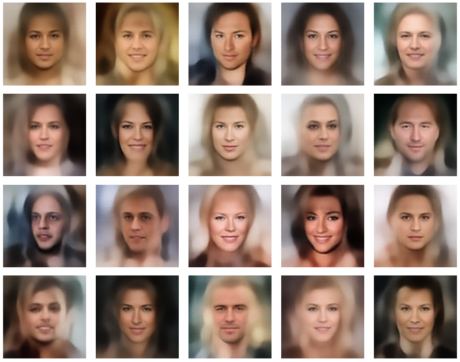
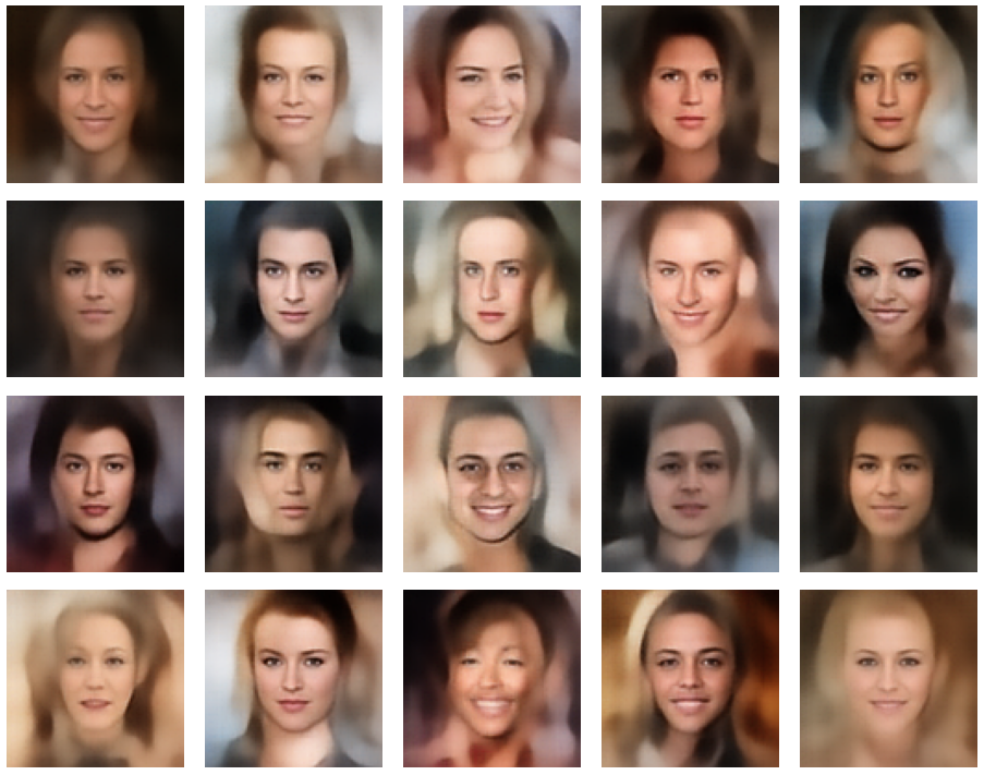
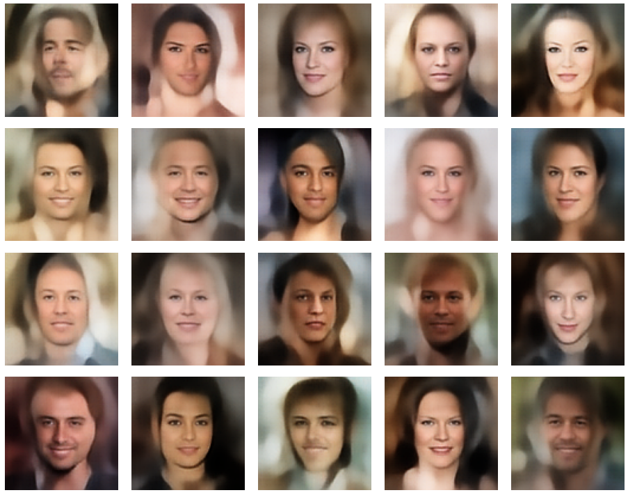
These ellipses with axes along the coordinate axes are relatively easy to handle. They can be used for vector creation. But they require a full PCA transformation of the MND-distribution, a PCA-analysis for complexity reduction and an application of the inverse PCA-transformation. The plot below shows the point-density compared to a 2.2-σ-confidence ellipses. The orange points are the results of a proper statistical numerical vector generation algorithm based on a PCA-transformation of the MND.

See my post quoted above for the application of a PCA-transformation of the multidimensional MND for vector creation.

However, we get the impression that we could also use these rotated ellipses in projections of the MND onto coordinate planes of the original latent space system directly to impose limiting conditions on the component values of statistical vectors pointing to an inner regions of the MND. Of course, a generated statistical vector must then comply with the conditions of all such ellipses. This requires an analysis and combined use of the ellipses of all of the subordinate BNDs of a the original MND during an iterative or successive definition of the values for the vector components.

Objective of this post series

In my last post about CAEs (see the link given above) I have explicitly asked the question whether one can avoid performing a full PCA-transformation of the MND when creating statistical vectors pointing to a defined inner region of a MND.

The objective of this post series is to prove the answer: Yes, we can. And we will use the BNDs resulting from projections of the original MND onto coordinate planes. We will in particular explore the n*(n-1)/2 the properties of the BNDs’ confidence ellipses. As said: These ellipses are rotated against the coordinate system’s axes. We will have to deal with this in detail. We will also use properties of their 1-dimensional marginal distributions (projections onto the coordinate axes, i.e. the V_j.)

In addition we need to prepare a variety of formulas before we are able to define numerical procedure for the vector generation without a full PCA-transformation of the MND with around 100,000 vectors. Some of the derived formulas will also allow for a deeper insight into how the multiple BNDs of a MND are related between each other and with confidence hypersurfaces of the MND.

Ellipses in general lead to equations governed by quadratic or fourth power polynomials. We will in addition use some elementary correlation formula from statistics and for some exercises a simple optimization via derivatives. The series can be regarded as an excursion into some of the math which governs bivariate distributions resulting from a MND.

As MNDs may also be the result of other generative Machine Learning algorithms in respective latent spaces, the whole approach to statistical vector generation for such cases should be of general interest. Note also that the so called “central limit theorem” almost guarantees the appearance of MNDs in many multivariate datasets with sufficiently large samples and value dependencies on many singular observations.

Distributions of a variety of variables may result in a MND if the variables themselves depend on many individual observables with limited covariance values of their distributions. In particular pairwise linearly correlated Gaussian density distributions individual variables (seen as vector components) may constitute a MND if the conditional probabilities fulfill some rules. We will see a glimpse of this in 2 dimensions when we analyze integrals over Gaussians in the bivariate normal case.

Other approaches to statistical vector generation?

Well, we could try to reconstruct the multidimensional density function of the MND. This is a challenge which appears in some problems of pure statistics, but also in experimental physics. See e.g. a paper of Rafey Anwar, Madeline Hamilton, Pavel M. Nadolsky (2019, Department of Physics, Southern Methodist University, Dallas; https://arxiv.org/pdf/1901.05511.pdf). Then we would have to find the elements of the (inverse) covariance matrix or – equivalently – the elements of a multidimensional rotation matrix. But the most efficient algorithms to get the matrix coefficients again work with projections onto coordinate planes. I prefer to use properties of the ellipses of the bivariate distributions directly.

Note that using the multidimensional density function of the MND directly is not of much help if we want to keep the vectors’ end points within a defined multidimensional inner region of the distribution. E.g.: You want to limit the vectors to some confidence region of the MND, i.e. to keep them inside a certain multidimensional ellipsoidal contour hyper-surface. The BND-ellipses in the coordinate planes reflect the multidimensional ellipsoidally shaped contour hyperplanes of the full distribution. Actually, when we vertically project a multidimensional hyperplane onto a coordinate plane then the outer 2-dim border line coincides with a contour ellipse of the respective BND. (This is due to properties of a MND. We will come back to this in a future post.) The problem of proper limiting individual vector component values thus again is best solved by analyzing properties of the BNDs.

Steps, methods, mathematical level

As a first step I will, for the sake of completeness, write down the formula for a multivariate normal distribution, discuss a bit its mathematical construction from uncorrelated univariate normal distribution. I will also list up some basic properties of a MND (without proof!). These properties will justify our approach to create statistical vectors pointing into a defined inner region of the MND by investigating projected contour ellipses of all subordinate BNDs. As a special aspect I want to make it at least plausible, why the projected contour ellipses define infinitesimal regions of the same relative probability level as their multidimensional counterparts – namely the multidimensional ellipsoidal hypersurfaces which were projected onto coordinate planes.

Then as a first productive step I want to motivate the specific mathematical form of the probability density function [p.d.f] of a bivariate normal distribution. In contrast to many of the math papers I have read on the topic I want to use a symmetry argument to derive the basic form of the p.d.f. I will point out an important, but plausible assumption about conditional distributions. An analogous assumption on the multidimensional level is central for the properties of a MND.

As the distributions V_j and V_k can be correlated we then want to understand the impact of the correlation coefficients on the parameters of the 2-dimensional density function. To achieve this I will again derive the density function by using our previous central assumption and some simple relations between the expectation values of the constituting two univariate distributions in the linear correlation regime. This concludes the part of the series where we get familiar with BNDs.

Furthermore we are interested in features and consequences of the 2-dimensional density functions. The contour lines of the 2-dim density function are ellipses – rotated by some specific angle. I will look at a formal mathematical process to construct such ellipses – in particular confidence ellipses. I will refer to the results Carsten Schelp has provided in an Internet article on this topic.

His construction process starts with a basic ellipse, which I will call base correlation ellipse [BCE]. The length of the axes of this ellipse are eigenvalues of the covariance matrix of the standardized marginal distributions constituting the BND. The main axes of this elementary ellipse are in addition aligned with the two selected axes of a basic Euclidean coordinate system in which the bivariate distribution is defined. The length of the BCE’s main axes can be shown to depend on the correlation coefficient for the two vector component distributions V_j and V_k. This coefficient also appears in the precision matrix of the BND. Points on the base correlation ellipse can be mapped with two steps of an affine transformation onto points on the real contour ellipses, in particular to points of the confidence ellipses.

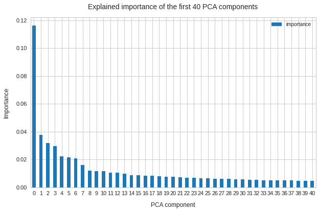
The whole construction process is not only of immense help when designing visualization programs for the contour ellipses of our distribution with many (around 100,000) individual vectors. The process itself gives us some direct geometrical insights. It also helps to avoid finding a numerical solution of the usual eigenvector-problems when answering some specific questions about the rotated contour ellipses. Normally we solve an eigenvalue-problem for the covariance matrix of the multi- or the many subordinate bi-variate distributions to get precise information about contour ellipses. This corresponds to a transformation of the distributions to a new coordinate system whose axes are aligned to the main axes of the ellipses. Numerically this transformation is directly related to a PCA transformation of the vector distributions. However, such a PCA-transformation can be costly in terms of CPU time.

Instead, we only need a numerical determination of all the mutual the correlation coefficients of the univariate marginal distributions of the MND. Then the eigenvalue problem on the BND-level is already analytically solved. We therefore neither perform a full numerical PCA analysis of the MND and multidimensional rotation of the vectors of around 100,000 samples. Nor do we analyze explained variance ratios to determine the most important PCA components for dimensionality reduction. We neither need to perform a numerical PCA analysis of the BNDs.

Most important: Our problem of vector generation is formulated in the original latent space coordinate system and it gets a direct solution there. The nice thing is that Schelp’s construction mechanism reduces the math to the solution of quadratic polynomial equations for the BNDs. The solutions of those equations, which are required for our ultimate purpose of vector generation, can be stated in an explicit form.

Therefore, the math in this series will mostly remain on high school level (at least at a level given when I was young). Actually, it was fun to dive back into exercises reminding me of school 50 years ago. I hope the interested reader has some fun, too.

Solutions to some particular problems with respect to the confidence ellipses of the MND’s BNDs

In particular we will solve the following problems:

Problem 1: The two points on the BCE-ellipse with the same v_j-value are not mapped onto points with the same v_j-value on the confidence ellipse. We therefore derive the coordinates of points on the BCE-ellipse that give us one and the same v_j-value on the real confidence ellipse.
Problem 2: Plots for a real MND vector distribution indicate that all (n-1) confidence ellipses of distribution pairs of a common V_j with other marginal distributions V_k (for the same confidence level and with k ≠ j) have a common tangent parallel to one coordinate axis. We will derive the value of a maximum v_j-value for all ellipses of (j,k)-pairs of vector component distributions. We will prove that it is identical for all k. This will define the common interval of allowed v_j-component-values for a bunch of confidence ellipses for all (V_j, V_k)-pairs with a common V_j.
Problem 3: The BCE-ellipses for a common j-, but different k-values depend on different values for the correlation coefficients ρ_j,k of V_j with its various V_k counterparts. Therefore we need a formula that relates a point on the BCE-ellipse leading to a concrete v_j-value of the mapped point on the confidence ellipse of a particular (V_j, V_k)-pair to respective points on other BCE-ellipses of different (V_j, V_m)-pair with the same resulting v_j-value on their confidence ellipses. I will derive such a formula. It will help us to apply multiple conditions onto the vector component values.
Problem 4: As a supplemental exercise we will derive a mathematical expression for the size of the main axes and the rotation angle of the ellipses. We should, of course, get values that are identical to results of the eigenwert-problem for the correlation matrix (describing a PCA coordinate transformation). This gives us additional confidence in Schelps’ approach.

In the end we can use our results to define a numerical algorithm for the direct creation of vectors pointing to a defined inner region of the multivariate normal distribution. As said, this algorithms does not require a costly PCA transformations of the full MND or many, namely n*(n-1)/2 such PCA-transformations of its BNDs.

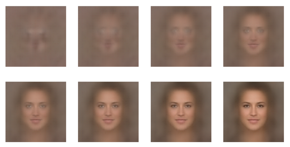
I intend to visualize all results with the help of a concrete example of a multivariate example distribution created by a CAE for the CelebA dataset. The plots will use Schelp’s construction algorithm for the confidence ellipses extensively.

Conclusion and outlook

Convolutional Autoencoders create approximate multivariate normal distributions [MND] for certain input data (with Gaussian pattern properties) in their latent space. MNDs appear in other contexts of machine learning and statistics, too. For evaluation and generative purposes one may need statistical vectors with end points inside a defined multidimensional hypersurface corresponding to a certain confidence level and a certain constant density value of the MND’s density function. These hypersurfaces are multidimensional ellipsoids.

We have the hope that we can use mathematical properties of the MND’s subordinate bivariate normal distributions [BNDs] to create statistical vectors with end points inside the multidimensional confidence ellipsoids of a MND. Typically such an ellipsoid resides off the origin of the latent space’s coordinate system and the ellipsoid’s main axes are rotated against the axes of the coordinate system. We intend to base the confining conditions on the components of the aspired statistical vectors on correlation coefficients of the marginal vector component distributions. Our numerical algorithm should avoid a full PCA-transformation of the multidimensional vector distribution.

In the next post of this series I give a formula for the density function of a multivariate normal distribution. In addition I will list up some basic properties which justify the vector generation approach via bivariate normal distributions.

Autoencoders and latent space fragmentation – X – a method to create suitable latent vectors for the generation of human face images

Posted on 3. June 2023 by eremo

My present post series explores options to use a standard convolutional Autoencoder [AE] for the creation of images with human faces. The face generation should based on random input to the AE’s Decoder. On our quest for a suitable method we have meanwhile learned a lot about other aspects of Autoencoders, vector distributions in multi-dimensional latent spaces and generative methods for our special case:

Methods to create statistical latent vectors [z-vectors] as input for the AE’s Decoder must be chosen carefully. Among other things: It is difficult to create a bunch of random vectors which cover wider areas in the vastness of a multidimensional space. So the z-vector creation must be adjusted to specific requirements.
After having been trained with CelebA images a convolutional AE fills a limited and coherent region in the latent space with z-points for the training images. This latent space region appears to be critical for successful image creation: Statistically generated z-vectors should point to this region. The core of the z-point distribution gets filled relatively densely.
A convolutional AE maps human face images onto an approximate multivariate normal distribution. This gives the inner core of the z-point distribution the structure of a multidimensional ellipsoid. The projections of this ellipsoid onto 2-dimensional coordinate planes show characteristic nested elliptic contour lines.
As the main axes of these ellipses were inclined with different angle towards the axes of chosen coordinate planes we concluded that linear correlations mark average dependencies between the z-vector components. Limiting conditions imposed by these correlations must also be fulfilled by z-vectors used as the Decoder’s input.

See previous posts in this series for more details. In particular, the last 2 posts

Autoencoders and latent space fragmentation – IX – PCA transformation of the z-point distribution for CelebA

Autoencoders and latent space fragmentation – VIII – approximation of the latent vector distribution by a multivariate normal distribution and ellipses

have shown that the density distribution for the z-points really exhibits elliptic contour lines in the original coordinate system of the latent space and (!) in the target coordinate system of a PCA transformation.

In this post we use our gathered knowledge: I present a first simple method to generate z-vectors which point to the latent space region filled by z-points for CelebA images. These z-vectors will fulfill the general and limiting elliptic conditions for their components.

Decomposing the full problem of latent vector generation into a sequence of 2-dimensional problems

The nice thing about multivariate Gaussian distributions with linear correlations between the vector components is the following: We can reduce the problem of choosing proper component values to a series of 2-dimensional restrictions. Firstly we can use characteristic properties of the Gaussian distribution for each component. And secondly we can use confidence ellipses in 2-dimensional coordinate planes to restrict the component values to allowed intervals.

Ellipses are most easy to handle when their axes are aligned with the axes of the coordinate system in which we describe them. So, let us assume that we know an affine transformation T to a new coordinate system which also has orthogonal axes and supports the following special transformation properties for a multivariate normal density distribution:

T maps nested elliptic contour lines of the multidimensional density distribution and in particular confidence ellipses for component pairs in the original coordinate system to nested elliptic contours and confidence ellipses in the new coordinate system.
Taligns the centers of the transformed ellipses with the origin of the new coordinate system.
T aligns the main axes of the mapped ellipses with the axes of the new coordinate system.
T is reversible.

How could we then use the transformed data for vector-creation?

In the new coordinate system, a contour ellipse in a chosen coordinate plane for the axes-indices (i, j) may have main diameters of size

d1 = 2 * a and d2 = 2 * b.

We then can first select a random v_i value to fall into a range [-a * fact, a * fact].

– fact * a < v_i < fact * a

With fact being a proper factor. This factor defines a confidence level in the new coordinate system. With the value of v_i fixed and b being the half-diameter in the orthogonal direction the correlation condition for the z-point distribution says that the v_j value must fall into an interval [-c, c] defined by:

-c < v_j < c,
with c = b * fact * sqrt(1 – x**2 / (fact * a)**2)

But within these limits we can again choose the v_j-value freely. Below I use a simple random-function for a constant probability density to pick a value.

However: It would not be enough to restrict the coordinates to the conditions of just one ellipse! The components of the created vectors must in parallel fulfill elliptic conditions for all of the possible pairs of vector-components. I.e. we may need to adapt the v_j values gained from the analysis of a fist 2D-ellipse to further conditions of other ellipses and component pairs. This can be achieved by an iteration. For z_dim = 256 this involves a total of 32640 checks and possible value-adaptions to each and all of the allowed value ranges.

In addition: The order by which the component-pairs and their conditions are investigated must be randomized to get real statistical vector distributions.

Eventually the resulting vector components must be re-transformed into the original coordinate system of the latent space.

The ellipse for the “core’s boundary” in the original coordinate system will be defined by the chosen confidence level of the ellipsoidal normal distribution. We saw already that a confidence level of σ = 2.0 defines the transition to outer regions of the z-point density distribution quite well.

This all sounds manageable by relative simple Python programs. But: Do we know a proper transformation T? Yes, we do: A PCA-transformation of the z-point density distribution has all the properties discussed above.

Using half maximum values after a PCA transformation of the z-point distribution

The last post proved that a PCA transformation maps ellipses onto ellipses for component pairs in the transformed PCA coordinate system. The advantage of the ellipses there is that their main axes are on average well aligned with the orthogonal PCA coordinate axes. Gaussians for the number density distribution per component are mapped to Gaussians for the new components in the transformed coordinate system. So, the basic idea for a proper z-vector generation is:

Take the multivariate normal z-point distribution for the training images in the AE’s latent space.
Apply a PCA analysis to diagonalize the correlation matrix and transform the z-vector components to the PCA coordinate system.
Use the ellipses in coordinate planes of the PCA coordinate system to create random z-vector components fulfilling all required conditions there.
Re-transform the resulting z-vector components into the original coordinate system of the latent space.

Point 3 in our method is covered by a numerical analysis of the Gaussians in the PCA-coordinate system. We determine the half-width numerically by analyzing the density distribution with the help of sampling intervals. This simple method has resolution limits related to the size of the sampling interval. This has consequences for PCA components with a small standard deviation. We saw already in the last posts that such distributions appear for higher PCA components at the lower end of the explained variance.

Does the suggested method work?

The convolutional AE we work with was defined in previous posts with 4 Conv2D layers in the Encoder and 4 Conv2DTranspose layers in Decoder. The number of latent space dimensions was z_dim = 256. The AE network was trained on CelebA images. I do not want to bore you with details of the codes for the creation of z-vectors consistent to the resulting elliptic conditions. It is all standard. The PCA-transformation can e.g. be taken from the sklearn-package.

I have applied a constant probability density to choose a random value within the allowed ranges for the component values of the aspired z-vectors in the PCA coordinate system. For the plots below I have used the most important 50 to 105 PCA components (out of 256). The plots include confidence ellipses on a level of σ = 2.2. I derived the confidence ellipses by directly evaluating the standard deviations of the transformed distribution data in all coordinate directions.

The first plot shows you such an ellipse for the coordinate plane corresponding to the first two, most important PCA components. The orange points mark 20 z-points defined by 20 randomly z-vectors fulfilling all elliptic conditions. The plot contains 120,000 z-points for images out of the 170,000 CelebA pictures used during training.

Generated statistical vectors in the PCA coordinate system

For elliptic contour lines see the last post before the present one in this series. The next plot shows the same generated 20 z-vectors for other component-combinations among the first 20 of the most important PCA-components. The plots contain a selection of 60,000 z-points.

The outer z-points points do not always indicate that we have elliptic contours in the denser core of the displayed 2-dimensional distributions. But see the last post for proofs that the inner core inside the red ellipse really displays elliptic contours. You see that all random vectors lie within the 2-σ-ellipses.

The next plot shows the generated z-vectors in the original coordinate system of the latent space. The component values were back-transformed from the PCA-system to the original coordinate system.

Generated statistical z-vectors after an inverse PCA transformation to the original coordinate system of the latent space

We get similar plots for other component pairs. And of course for other generated vectors.

Generated statistical z-vectors in the PCA coordinate system

Generated statistical z-vectors after an inverse PCA transformation to the original coordinate system of the latent space

Technically we have obviously achieved what we wanted: Our generated statistical vectors are distributed within the core of our multidimensional ellipsoid.

Note that this method fortunately works even when we use a limited number of the PCA components, only. This is due to intricate properties of a PCA transformation which guarantee that a back-transformation puts the resulting points close to the original ones even when we omit less important PCA components. I cannot discuss the math-details in this blog. You have to see scientific literature for this. An introduction is e.g. provided by https://arxiv.org/pdf/1404.1100.pdf.

For me this property of the PCA transformation was helpful when I ran into the resolution problem for a proper half-width of the Gaussians. Taking 256 components lead to errors as elliptic conditions for very narrow Gaussians were not properly defined and some of the created vectors left the allowed value ranges.

Resulting face images

Let us look at some results. First I want to remind you from where we started:

Failed trials with improper random z-vectors based on constant probability densities

A simple random generator used in the beginning was totally inapt to feed the AE’s Decoder with proper statistical z-vectors. And now – look at the following plots. They were produced for a varying number of PCA components between 50 and 120, 100000 statistically selected z-points within a 3 σ-level for the PCA-transformation and various factors 0.6 < fact < 0.8 used upon a half-width corresponding to a confidence level of 2.35 σ:

In some cases – for a higher number of PCA components – we even see smaller details of the face images and a reasonable transition to some kind of hairdo. Please remember that z_dim = 256 is a pretty low number for the latent space to cover the encoding of face details. And celebrities as covered by CelebA use make-up ….

In case you think the above result is not noteworthy: Please remember that we talk about a simple standard Autoencoder and not about a Variational Autoencoder and neither about a transformer based Autoencoder. No fancy additions to cost functions or special layers. And who ever has read the very instructive book of D. Foster on “Generative Deep Learning” (1st edition, O’Reilly) may compare his images to mine. And I have used a lower resolution of the original images than D. Foster. Just to motivate people to look a bit deeper into properties of data distributions in latent spaces.

Conclusion and outlook

We have come a lot closer to our objective of using a standard minimal Autoencoder for generative purposes. On our way, we got a much deeper understanding of the vector-distribution a trained AE creates in its latent space for human face images.

The method presented in this post to create reasonable statistical z-vectors still has its limits and there is a lot of open space for improvements. Attentive readers may e.g. ask: Why did he not use confidence ellipses directly? And why not the ellipses found in the original coordinate system of the latent space? And what about micro-correlations? And are there clusters for certain properties as the hair-color, sex, smiling, etc. in the multivariate z-point distribution in the AE’s latent space?

I will discuss these topics in further posts. In the meantime keep in mind that the basic point for turning a standard Autoencoder into a generative tool is to understand how it fills its latent space.

Note also that I myself have speculated in other posts of this blog that failures of using standard AEs for generative purposes may have their ultimate reason in the micro-structure of the z-point distribution. The present results render these previous ideas of mine plain wrong.

Links to previous posts of this series

Autoencoders and latent space fragmentation – IX – PCA transformation of the z-point distribution for CelebA

Autoencoders and latent space fragmentation – VIII – approximation of the latent vector distribution by a multivariate normal distribution and ellipses

Autoencoders and latent space fragmentation – VII – face images from statistical z-points within the latent space region of CelebA

Autoencoders and latent space fragmentation – VI – image creation from z-points along paths in selected coordinate planes of the latent space

Autoencoders and latent space fragmentation – V – reconstruction of human face images from simple statistical z-point-distributions?

Autoencoders and latent space fragmentation – IV – CelebA and statistical vector distributions in the surroundings of the latent space origin

Autoencoders and latent space fragmentation – III – correlations of latent vector components

Autoencoders and latent space fragmentation – II – number distributions of latent vector components

Autoencoders and latent space fragmentation – I – Encoder, Decoder, latent space

And before we forget it: Besides the Putler in the east there is also an extremist right-wing, semi-fascistic party in Germany on a record high support level in the population of 18%. This is a party which wants to stop all sanctions against the Russian aggressor in the ongoing war in Ukraine. You see the pattern behind this? This party is presently becoming bigger in number of supporters than the government leading social democrats. So, there is more at stake at present in Europe than the war in Ukraine. We need to defend our democracies with all the means of democracies. And its time to ask for more decisive legal action against a party which already is under observation of the German internal secret service.

Autoencoders and latent space fragmentation – IX – PCA transformation of the z-point distribution for CelebA

Posted on 31. May 2023 by eremo

This series of posts is about standard convolutional Autoencoders [AEs]. We wish to use the creative ability of an AE’s Decoder for the creation of human face images. We trained a relatively simple example AE on the CelebA data set. For the generation of new human face images we wanted to feed the Decoder with randomly created z-vectors in the AE’s latent space. As arbitrary latent vectors did not deliver reasonable images, we had a look at properties of the z-point distribution created in the latent space after training. And we found the z-vectors with end-points within this particular region indeed gave us some first reasonable images.

But during the first posts we also had to learn that it requires substantial effort to produce “randomly” created z-vectors which point to the coherent and confined latent space region populated by z-points for CelebA images. In addition we found that we obviously must fulfill complex correlation conditions between the latent vector components. In the last posts we have, therefore, investigated the structure of the latent space region populated for CelebA images a bit more closely. See:

Autoencoders and latent space fragmentation – VIII – approximation of the latent vector distribution by a multivariate normal distribution and ellipses

Autoencoders and latent space fragmentation – VII – face images from statistical z-points within the latent space region of CelebA

This gave us a somewhat surprising insight:

For our special case of human face images the density distribution of the z-points in the multidimensional latent space roughly resembled a multivariate normal distribution. The variables of this distribution were, of course, the components of the latent z-vectors (reaching from the origin of the latent space coordinate system to the z-points). The number density distributions for the values of the z-vector components could very well be approximated by Gaussian functions. In addition we found strong linear correlations between the z-vector components. This was completely consistent with diagonally oriented elliptic contour lines of the number density distribution for pairs of z-vector components in the respective coordinate planes. The angles between the ellipses’ axes and the axes of the (orthogonal) coordinate system varied.

In this post we test my thesis of a multivariate normal distribution in a different and more complicated way. If the number density distribution of the z-points for CelebA really is close to a multivariate normal distribution then we would expect that the contour lines of the 2-dimensional number density function for coordinate planes still are ellipses after a PCA transformation. Note that the coordinate planes then are planes of a new coordinate system (with orthogonal axes) moved and rotated with respect to the original coordinate system. We call the transformed coordinate system the “PCA coordinate system“. (It is clear the vector components must consistently be transformed with respect to the new coordinate axes.)

This test is much harder because asymmetries, imperfections and deviations from a normal distribution will become clearly visible. Nevertheless we shall see that the z-point distribution decomposes roughly in uncorrelated Gaussian number density (or probability) functions for the (transformed) components of the z-vectors – as expected.

Note that number density distributions can be interpreted as probability distributions after a proper normalization. To understand the results and implications of this post some basic knowledge about multivariate normal probability density distributions in multidimensional spaces is required. Transformation properties of such distributions are important. In particular the effect of a PCA or SVD transformation, which diagonalizes the Pearson correlation matrix, on a multivariate normal distribution, should be familiar: In the moved and rotated coordinate system original linear correlations between vector components disappear. The coordinate axes of the transformed coordinate system get aligned to the eigenvectors (and main axes) of the probability density distribution. In addition elliptic contour lines prevail and the main axes of the ellipses get aligned with the axes of the PCA coordinate system.

For valuable information in previous posts see the link list a the bottom of this article.

Imperfections in the multivariate normal distribution and their consequences for PCA

In our case the latent space had 256 dimensions. The real number density functions for the values of the (256) latent vector components did not always show the full symmetry of their Gaussian fits. Deviations appeared near the center and at the flanks of the individual distributions. Still we got convincing overall ellipses in contour plots of the probability density for selected pairs of components. But there were also relatively many points which lay in regions outside the 2 to 3 sigma confidence ellipses for these 2-dimensional distributions – and the distribution of the points there seemed to violate the elliptic symmetry.

A perfect multivariate normal distribution (with only linear correlations between its variables) decomposes into (seemingly) uncorrelated normal distributions for the new variables, namely the latent vector components in the transformed coordinate system of the latent space. The coordinate transformation corresponds to a diagonalization of the Pearson correlation matrix via finding orthogonal eigenvectors. So we should not only get ellipses after the PCA transformation. The main axes of the resulting ellipses should also be aligned with the coordinate axes of the new translated and rotated PCA coordinate system. (This is a standard feature of “uncorrelated” Gaussians).

Note that the de-correlation is a pure coordinate effect which does not eliminate the dependencies of the original variables. The new coordinates and the respective variables do not have the same meaning as the old ones. We “only” change perspectives such that the mathematical description of the multivariate distribution gets simpler. However, the ratios of the axes of the new ellipses depend on the axis-ratios of the old ellipses in the original standard coordinate system of the latent space.

When we translate and rotate a coordinate system to diagonalize the Pearson matrix of an imperfect multivariate normal distribution the coordinate axes may afterward not fully align with the main axes of the distribution’s inner core – and then we might get clearly visible asymmetries in z-point projections to coordinate planes. Note that points outside the inner core have a relatively large impact on the PCA transformation and especially on the rotation of the new axes with respect to the old ones.

Reduction of outer z-point contributions

Outer z-points often correspond to CelebA images with strong variations in the background. As these z-points have a large distance from the center of the distribution they have a heavy impact on a PCA transformation to eigenvectors of the Pearson matrix. Therefore, I eliminated some outer points from the distribution. I did this by deleting points with coordinate values smaller or bigger than a symmetric threshold in the outer flanks of the 256 Gaussian distributions – e.g.:

z_j < mu_j – fact * FHWM and z_j > mu_j + fact * FHWM.

With FHWM meaning the full width at the half maximum and mu_j being the center of the approximate Gaussian for the j-th vector component of the z-vectors. I tried multiple values of fact between 1.7 and 1.25.

One has to be careful with such an elimination process. Even though we set our limits beyond the 2 σ-level of the individual Gaussians ahead of the transformation, a step-wise consecutive elimination for all components reduces the number of surviving vectors significantly for small values of fact. The plots below correspond to a value of fact = 1.7 (with one discussed exception). This reduced the number of available vectors from originally 170.000 used during the AE’s training to 160.000. From this distribution a random sub-selection of 80,000 z-points was taken to perform the PCA transformation. I call the resulting sample of z-points the “reduced distribution” below. The results did not change much for a sub-selection of more points. The second reduction saved me some CPU-time, however.

PCA transformation of the z-point distribution – explained variance and cumulative importance

Below you see the explained variance ratio of the first 40 and the cumulative importance of the first 120 main components after a PCA transformation of the reduced z-point distribution. (The PCA-algorithm was based on the SVD-algorithm, as provided by the sklearn-package.)

We see that we need around 120 PCA components to explain 80% of the variance of the original z-point data. The contribution of the first 15 components is significant, but it is NOT really dominant. Interesting is also the step-wise decline of the first 10 components in a not so smooth curve.

I have in addition checked that the normalized Pearson correlation coefficient matrix was perfectly diagonalized. All off-diagonal values were smaller than 2.e-7 (which is consistent with error propagation) and the diagonal elements were 1.0 with an accuracy better than 8 eight digits after the decimal point. As it should be.

Gaussians per PCA-vector component?

We expect Gaussian number density functions for each of the z-vector components after the PCA coordinate transformation. The following line plots show the number density distributions (colored line) and a related Gaussian fit (dashed lines) per named vector-components after PCA-transformation. The first plot gives an overview over 120 PCA components:

We see that all distributions look similar to Gaussians. In addition the center of the distributions for all components are very close to or coincide with the origin of the PCA coordinate system. This is something we would expect for an original multivariate normal distribution before the PCA transformation to a new moved and rotated coordinate system: An affine transformation between coordinate systems with orthogonal axes maps Gaussians to Gaussians.

Components 0 and 1:

Components 2 and 3:

Components 4 and 5:

Components 6 and 7:

Components 8 and 9:

We see from these plots that component 3 shows values at the distributions’s flanks well above the values of its Gaussian fit. This may lead to deformed ellipses. In addition component 7 shows a slight asymmetry – probably triggering deviations both at the center and outer regions. Similar effects can be seen for other higher components – but not so pronounced. The chosen sampling interval (0.5) in the new coordinates did smear out small asymmetric wiggles in all distributions.

Ellipses?

Calculating approximate contour lines is CPU intensive. On my presently available laptop I had to focus on some selected examples for pairs of components of z-vectors in the transformed coordinate system. Experiments showed that the most critical components with respect to asymmetries were 2, 3, 7, 8.

Let us first look at combinations of the first 9 PCA components (0) with other components in the range between the 10th and 120th PCA component. Just scroll down to see more images:

The fatter lines represent confidence ellipses derived both from correlation data, i.e. elements of the normalized correlation coefficient matrix, and properties of the Gaussian distributions. See the last blog for details on the method of getting confidence ellipses from data of a probability distribution.

Ellipses for density distributions in coordinate planes for pars of the most important PCA components

Before you think that everything is just perfect we should focus on the most important 10 PCA components and their mutual pair-wise density distributions. We expect trouble especially for combinations with the components 2, 3 and 7.

Component 0 vs other components < 10

We see already here that asymmetries in the density distributions which appear relatively small in the gaussian-like curves per component leave their imprint on the elliptic curves. The contour lines are not always centered with respect to the overall confidence ellipses.

Component 1 vs other components < 10

Component 2 vs other components < 10

The plot for components 2 and 3 was based on fact = 1.35 instead of fact = 1.7. See a section below for more information.

Component 3 vs other components < 10

Component 4 vs other components < 10

Component 5 vs other components < 10

Component 6 vs other components < 10

Component 7 vs other components < 10

Component 8 vs other components < 10

Component 9 vs other components < 10

Ellipses for other seected component pairs

Comments

The z-point distribution is rather close to a multivariate normal distribution, but it is not perfect. The PCA transformation revealed clearly that the center of the overall z-point distribution does not completely coincide with the centers of the individual density distributions for the z-vector components. And not all individual curves are fully symmetrical. Some plots show the expected ellipses, but not fully centered. We also see signs of non-linear correlations as not all ellipses show a complete alignment with the axes of the PCA coordinate system.

The impact of outer z-points becomes obvious when we compare plots for the component pair (2, 3) for different values of fact. The plots are for fact = 1.35, 1.45, 1.55, 1.7 and fact = 1.8 (in this order from left to right and downward). (Regarding z-point elimination the fact-values correspond to 122000, 138000, 149000, 159000 and 164000 remaining z-points.)

The flips in the left-right orientation between some of the plots can be ignored. They depend on random aspects of the transformations and plotting routines used.

We see that z-points (for some some strange images) which have a large distance from the center of the distribution have a major impact on the central density distribution. 10% of the outer points influence the orientation of the central ellipses by their coordinates – although these outer points are not part of the inner core of the distribution.

BUT: Overall we find the effect we wanted to see. The elliptic contours are clearly visible and most of them are aligned with the axes of the PCA coordinate system and the main axes of the confidence ellipses for the z-point distribution in the PCA coordinate system. The inner core is aligned with the axes of the coordinate system even for the critical PCA components 2 and 3, when we omit between 12% and 25% of the points (outside a 3 σ-level).

This means: The PCA transformation confirms that an inner core of the z-point distribution is well described by a multivariate normal distribution – with linear correlations between the number density distributions for various components.

This is an interesting finding by itself.

Conclusion

The last and the present post of this series have shown that a convolutional AE maps human face images of the CelebA data set to a multivariate normal distribution in its multidimensional latent space. Although this is interesting by itself we must not forget our ultimate goal – namely to generate random z-vectors which should deliver us reasonably human face images by the AE’s Decoder. But the results of our analysis provide solid criteria to generate such vectors fulfilling complex correlation conditions.

We can now define statistical generation methods which restrict the components of our aspired random z-vectors such that the resulting z-points lie within regions surrounded by confidence ellipses of the multivariate normal distribution. One such method is the topic of the next post.

Autoencoders and latent space fragmentation – X – a method to create suitable latent vectors for the generation of human face images

Links to other posts of this series

Autoencoders and latent space fragmentation – VIII – approximation of the latent vector distribution by a multivariate normal distribution and ellipses

Autoencoders and latent space fragmentation – VII – face images from statistical z-points within the latent space region of CelebA

Autoencoders and latent space fragmentation – VI – image creation from z-points along paths in selected coordinate planes of the latent space

Autoencoders and latent space fragmentation – V – reconstruction of human face images from simple statistical z-point-distributions?

Autoencoders and latent space fragmentation – IV – CelebA and statistical vector distributions in the surroundings of the latent space origin

Autoencoders and latent space fragmentation – III – correlations of latent vector components

Autoencoders and latent space fragmentation – II – number distributions of latent vector components

Autoencoders and latent space fragmentation – I – Encoder, Decoder, latent space

Autoencoders and latent space fragmentation – VI – image creation from z-points along paths in selected coordinate planes of the latent space

Posted on 30. April 2023 by eremo

It is well known that standard (convolutional) Autoencoders [AEs] cause problems when you want to use them for creative purposes. An example: Creating images with human faces by feeding the Decoder of a suitably trained AE with random latent vectors does not work well. In this series of posts I want to identify the cause of this specific problem. Another objective is to circumvent some of the related obstacles and create reasonably clear images nevertheless. Note that I speak about standard Autoencoders, not Variational Autoencoders or transformer based Encoder/Decoder-systems. For basic concepts, terms and methods see the previous posts:

Autoencoders and latent space fragmentation – I – Encoder, Decoder, latent space
Autoencoders and latent space fragmentation – II – number distributions of latent vector components
Autoencoders and latent space fragmentation – III – correlations of latent vector components
Autoencoders and latent space fragmentation – IV – CelebA and statistical vector distributions in the surroundings of the latent space origin
Autoencoders and latent space fragmentation – V – reconstruction of human face images from simple statistical z-point-distributions?

So far I have demonstrated that randomly generated vectors most often do not hit the relevant regions in the AE’s latent space – if we do not take some data specific precautions. A relevant region is a confined volume which a trained Decoder fills with z-points for its training objects after the training has been completed. z-points and corresponding latent vectors are the result of an encoding process which maps digitized input objects into the latent space. Depending on the data objects we may get multiple relevant regions or just one compact region. In the case of a convolutional AE which I had trained with the CelebA dataset of human face images I found single region with a rather compact core.

In this post I want to create statistical latent vectors whose end-points are located inside the relevant region for CelebA images. Then I will create images from such latent vectors with the help of the AE’s Decoder. My hope is to get at least some images with clearly visible human faces. The basic idea behind this experiment is that the most important features of human faces are encoded by a few dominant vector components defining the overall position and shape of the multidimensional z-point region for CelebA images. We will see that the theory is indeed valid: Here is a first example for a vector pointing to an outer area of the core region for CelebA images in the latent space:

Our AE is a convolutional one. The number of latent space dimensions N was chosen to be N=256.
Note: We are NOT using a Variational Autoencoder, but a simple standard Autoencoder. The AE’s properties were discussed in previous posts.

What have we found out so far?

The Encoder of the convolutional AE, which I had trained with the CelebA dataset, mapped the human face images into a compact region of the latent space. The core of the created z-point distribution was located within or very close to a tiny hyper-volume of the latent space spanned by only a few coordinate axes. The confined multi-dimensional volume occupied by most of the z-points had an overall ellipsoidal shape with major extensions along a few main axes. We saw that some of the coordinates of the CelebA z-points and the components of the corresponding latent vectors were strongly correlated. In addition the value range of each of the latent vector components had specific individual limits – confining the angles and lengths of the vectors for CelebA. Therefore we had to conclude:

Whenever we base our method to create statistical vectors on the assumptions

that one can treat the vector components as independent statistical variables
that one can assign statistical values to the components from a common real value interval

the vectors will almost certainly not point to the relevant region. In addition one has to take into account unexpected mathematical properties of statistical vector distributions in high dimensional spaces. See the previous posts for more details. Indeed we could show that such a vector generation method missed the CelebA region.

Objective of this post

In this post I want to use some of the knowledge which we have gathered about the latent vector distribution for CelebA images. We shall use a very simple approach to probe the image reconstruction abilities of the Decoder for a defined variety of z-points:

We restrict the vectors’ component values such that most of the vectors point to the region formed by the bulk of CelebA z-points. To achieve this we define straight line segments which cross the ellipsoidal region of CelebA z-points. This is possible due to the known value intervals which we have identified for each of the components in a previous post. Then we place some artificial z-points onto our line segments. At least some of these z-points will fall into the relevant CelebA region. We then let the Decoder reconstruct images for the latent vectors corresponding to these z-points.

In some cases our paths will even respect some major component correlations, but for some paths I will explicitly disregard such correlations. Nevertheless our rather simple restrictions imposed on the vector-component values will already enable us to produce images with clearly recognizable face features.

Among other things our results confirm the idea that the real pixel correlations for basic face features are represented by relatively narrow limits for the angles and lengths of respective latent vectors. The extension and shape of the bulk region of CelebA z-points is defined by only a few latent vector components. These components apparently encode a prescription for the (convolutional) Decoder to create face features by a superposition of some elementary patterns extracted during the AE’s training.

A path from the latent space origin to the center of the relevant z-point region

How do we restrict latent vectors to the required value ranges? In the 2nd post we have seen that the number distribution curve for the values of each of the latent vector components was very similar to a Gaussian. We have identified the mean value and average value range for each component by analyzing its specific distribution curve. The mean values gave us the coordinates of the center of the relevant latent space region. In addition we, of course, know the coordinates of the origin of the latent space. So, for a first test, let us create a multi-dimensional line segment between the origin and the center of the CelebA z-point distribution. And let the A’s Decoder create images for latent vectors pointing to some intermediate z-points along this path.

The following plots show orthogonal projections of 5000 CelebA z-points (in blue) onto some 2-dimensional planes spanned by two selected coordinate axes. The yellow dot indicates the origin. The orange dot the center of the z-point distribution. Red dots indicate coordinates of points along the straight path between the origin and the distribution center.

Please, take note of the different scales on the x- and y-axes. Some distributions are much more elongated than the scaled images show. That some paths appear shorter than others is due to the projection of the diagonal line through the multi-dimensional space onto planes which are differently oriented with respect to this line. A simple 3D analog should make this clear. Some small wiggles in the positions of the red dots are due to resolution problems of the plot on the browser interface. We also see a reflection of the fact that the origin is located in a border region of the bulk.

Below you see a plot which shows the path in higher resolution (projected onto a particular plane):

Again: Take note of the different axis scales. The blue dot distribution is much more stretched in C1-direction than it appears in the plot.

Ok, now we have a multidimensional path and six well defined latent vectors for the end and intermediate points on this path. So let us provide these vectors as input to the our AE’s Decoder. The resulting images look like:

Success! Images in the surroundings of the center show a clearly visible face. And we also see: The average face at the center of the z-point distribution is female – at least according to the CelebA dataset. 🙂 However: In the vicinity of the origin of the latent space we get no images with reasonable face features.

Images along a path within a selected coordinate plane for two dominant vector components

I choose a different path within the plane spanned by the coordinates axes 151 and 195 now. This is depicted in the plot below:

A look into the second post shows you that the components 151, 195 were members of the group of dominant components. Those were components for which the number distribution showed a mean value at some distance from the origin of the latent space and also had a half-width bigger than 1.0 (as most of the other components). The images reconstructed by the Decoder from the latent vectors are:

Hey, we get some variation – as expected. Now, let us rotate the path in the plane:

Not so much of a difference. But we have learned that a variation of some vector component values within the allowed range of values may give us already some major variation in the faces’ expressions.

Images for other coordinate planes

The following images show the variations for paths in other coordinate planes. All of the paths have in common that they pass the center of the CelebA bulk region. For the first 4 examples I have kept the path within the core region of CelebA z-points. The last images show images for paths with z-points at the core’s border regions or a bit outside of it.

Plane axes: 5, 8

Plane axes: 17, 180

Plane axes: 44, 111

Plane axes: 55, 56

Plane axes: 15, 242

Plane axes: 58 202

Plane axes: 68, 178

Plane axes: 177, 202

Plane axes: 180, 242

The images for z-points farther away from the bulk’s center give you more interesting variations. But obviously in the outer areas of the CelebA region correlations between the latent vector components get more important when we want to avoid irregular and unrealistic disturbances. All in all we also get the impression that a much more subtle correlation of component values is a key for the reproduction of realistic transitions for the hairdos presented in the CelebA images and the transition to some realistic background patterns. The components of our latent vectors are still too uncorrelated for such details and an appropriate superposition of micro-patterns in the images created by the Decoder.

Conclusion

This blog shows that we do not need a Variational Autoencoder to produce images with recognizable human faces from statistical latent vectors. We can get image reproductions with varying face features also from the Decoder of a standard convolutional Autoencoder. A basic requirement seems to be that we keep the vector components within reasonable value intervals. The valid component specific value ranges are defined by the shape of the compact hyper-volume, which an AE’s Encoder fills with z-points for its training objects. So we need to construct statistical latent vectors which point to this specific sub-region of the latent space. Vectors with arbitrary components will almost certainly miss this region and give no interpretable image content.

In this post we have looked at vectors defining z-points along specific line segments in the latent space. Some of the paths were explicitly kept within the inner core regions of the z-point-distribution for CelebA images. From these z-points the most important face features were clearly reconstructed. But we also saw that some micro-correlations of the latent vector components seem to control the appearance of the background and the transition from the face to hair and from the hair to the background-environment.

I have not yet looked at line segments which do not cross the center of the bulk of the z-point distribution for CelebA images in the latent space. But in the next post

Autoencoders and latent space fragmentation – VII – face images from statistical z-points close to the latent space region of CelebA

I first want to look at z-points for which we relatively freely vary the component values within ranges given by the respective number distributions.

Autoencoders and latent space fragmentation – V – reconstruction of human face images from simple statistical z-point-distributions?

Posted on 24. April 2023 by eremo

In this post series we have so far studied the distribution of latent vectors and z-points for CelebA images in the latent space of an Autoencoder [AE]. The CelebA images show human faces. We want to reconstruct images with new faces from artificially created, statistical latent vectors. Our latent space had a number dimensions N=256. For basics of Autoencoders, terms like latent space, z-points, latent vectors etc. see the first blog of this series:

Autoencoders and latent space fragmentation – I – Encoder, Decoder, latent space

During the experiments and analysis discussed in the other posts

Autoencoders and latent space fragmentation – II – number distributions of latent vector components
Autoencoders and latent space fragmentation – III – correlations of latent vector components
Autoencoders and latent space fragmentation – IV – CelebA and statistical vector distributions in the surroundings of the latent space origin

we have learned that the multi-dimensional latent space volume which the Encoder of a convolution AE fills densely with z-points for CelebA images has a special shape and location. The bulk of z-points is confined to a multi-dimensional ellipsoid which is relatively small. Its center has a position, which does not coincide with the latent space’s origin. The bulk center is located within or very close to a hyper-sub-volume spanned by only a few coordinate axes.

We also saw also that we have difficulties to hit this region by artificially created z-points via latent vectors. Especially, if the approach for statistical vector generation is a simple one. In the beginning we had naively assumed that we can treat the vector components as independent variables. We assigned each vector component values, which we took from a value-interval [-b, b] with a constant probability density. But we saw that such a simple and seemingly well founded method for statistical vector creation has a variety of disadvantages with respect to the bulk distribution of latent vectors for CelebA images. To name a few problems:

The components of the latent vectors for CelebA images are correlated and not independent. See the third post for details.
If we choose b too large (&gt. 2.0) then the length or radius values of the created vectors will not fit typical radii of the CelebA vectors. See the 2nd post for details.
The generated vectors only correspond to z-points which fill parts of a thin multi-dimensional spherical shell within the cube filled by points with coordinate values -b < x_j < +b. This is due to mathematical properties of the distribution in multi-dimensional spaces. See the second post for more details.

Optimal parameter values are 1.0 < b < 2.0, just to guarantee at least the right vector length. However, due to the fact that the origin of the latent space is located in a border region of the CelebA bulk z-point distribution, most points will end up outside the bulk volume.

In this post I will show you that our statistical vectors and the related z-points do indeed not lead to a successful reconstruction of images with clearly visible human faces. Afterward I will briefly discuss whether we still can have some hope to create new human face images by a standard AE’s Decoder and statistical points in its latent space.

Relevant values of parameter b for the interval from which we choose statistical values for the vector components

What does the number distribution for the length of latent CelebA vectors look like? For case I explained in the 2nd post of this series we get:

For case II:

Now let me remind you of a comparison with the lengths of statistical vectors for different values of b:

See the 2nd post of this series for more details. Obviously, for our simple generation method used to create statistical vectors a parameter value b = 1.5 is optimal. b=1.0 an b=2.0 mark the edges of a reasonable range of b-values. Larger or smaller values will drive the vector lengths out of the required range.

Image reconstructions for statistical vectors with independent component values x_j in the range -1.5 < x_j < 1.5

I created multiples of 512 images by feeding 512 statistical vectors into the Decoder of our convolutional Autoencoder which was trained on CelebA images (see the 1st and the 2nd post for details). The vector components x_j fulfilled the condition :

-1.5 ≤ x_j ≤ 1.5, for all j in [0, 256]

The result came out to be frustrating every time. Only singular image showed like outlines of a human face. The following plot is one example out of series of tenths of failures.

And this was an optimal b-value! 🙁 But due to the analysis of the 4th post in this series we had to expect this.

Image reconstructions for statistical vectors with independent component values x_j in the range -1.0 < x_j < 1.0

The same for

-1.0 ≤ x_j ≤ 1.0, for all j in [0, 256]

Image reconstructions for statistical vectors with independent component values x_j in the range -2.0 < x_j < 2.0

The same for

-2.0 ≤ x_j ≤ 2.0, for all j in [0, 256]

Image reconstructions for statistical vectors with independent component values in the range -5.0 < x_j < 5.0

If you have read the previous posts in this series then you may think: Some of the component values of latent vectors for CelebA images had bigger values anyway. So let us try:

-1.0 ≤ x_j ≤ 1.0, for all j in [0, 256]

And we get:

Although some component values may fall into the value regions of latent CelebA vectors most of them do not. The lengths (or radii) of the statistical vectors for b=5.0 do not at all fit the average radii of latent vectors for CelebA images.

What should we do?

I have described the failure to create reasonable images from statistical vectors in some regions around the origin of the latent space also in other posts on standard Autoencoders and in posts on Variational Autoencoders [VAEs]. For VAEs one enforces that regions around the origin are filled systematically by special Encoder layers.

But is all lost for a standard Encoder? No, not at all. It is time that we begin to use our knowledge about the latent z-point distribution which our AE creates for CelebA images. As I have shown in the 2nd post it is simple to get the number distribution for the component values. Because these distributions were similar to Gaussians we have rather well defined value regions per component which we can use for vector creation. I.e. we can perform a kind of first order approximation to the main correlations of the components and thus put our artificially created values inside the densely populated bulk of the z-point region for CelebA images. If that region in the latent space has a meaning at all then we should find some interesting reconstruction results for z-points within it.

We can do this even with our simple generation method based on constant probability densities, if we use individual value regions -b_j ≤ x_j ≤ b_j for each component. (Instead of a common value interval for all components). But even better would be Gaussian approximations to the real number distributions for the component values. In any case we have to restrict the values for each component much stronger than before.

Conclusion

What we already had expected from previous analysis became true. A simple method for the creation of statistical latent vectors does not give us z-points which are good for the creation of reasonable images by a trained AE’s Decoder. The simplifications

that we can treat the component values of latent vectors as independent variables
and that we can assign the components x_j values from a common interval -b ≤ x_j &le b

cause that we miss the bulk region in the AE’s latent space, which gets filled by its trained Encoder. We have demonstrated this for the case of an AE which had been trained on images of human faces.

In the next post

Autoencoders and latent space fragmentation – VI – image creation from z-points along paths in selected coordinate planes of the latent space

I will show that even a simple vector creation can give us latent vectors within the region filled for CelebA images. And we will see that such points indeed lead to the reconstruction of images with clearly visible human face images by the Decoder of a standard AE trained on the CelebA dataset.