Some readers may remember a post series I have written in this blog about the reconstruction of human faces with a CNN-based Autoencoder. I could show that the information in the latent space of the Autoencoder is given in form of a core of a Multivariate Normal Distribution [MVN].
This did not surprise too much as there are good reasons to assume that facial features on average, but in particular across rather symmetric celebrity faces follow Gaussian distributions. Hundreds of encoded features together form a MVN-distribution in a latent space of hundreds of dimensions. The Encoder part of a CNN-based Autoencoder is a pattern extraction machine – and there is no simpler pattern in multiple dimensions than a (off-center) MVN! A MVN’s multidimensional and concentric contour surfaces are ellipsoids, which have an algebraic description in form of quadratic forms. In case of the MVN defined by the inverse of the covariance matrix.
During the named series, I have extensively used that fact that the projections of a multidimensional MVN down to a coordinate planes result in 2-dimensional bivariate MVNs. The elements of the (2×2)-covariance matrix of the various 2-dimensional projected distributions could simply be picked from (nxn) covariance matrix of the original MVN – by a simple selection process. I had taken this procedure as granted, as it had been claimed in some publications. And it worked very well … See e.g.
and links therein to other posts. The projection of course affects the (n-1)-dimensional ellipsoidal and concentric contour surfaces of a MVN and maps them onto (p-1)-dimensional contour ellipses of the projected 2-dimensional MVNs. For respective images see this post:
Last weeks I looked a bit deeper into the mathematics of orthogonal projections of multidimensional ellipsoids onto sub-spaces of the ℝn. It came a bit of a surprise to me that the math behind the projections of figures controlled by quadratic forms is relatively complicated. In the general case of the projection to a p-dimensional sub-space, the quadratic form matrix for the ellipsoidal hull of the projection image is a so called Schur complement of the original ellipsoid’s quadratic form matrix.
Fortunately, the relation between the inverse matrices of the quadratic forms for the ellipsoids could be established in a way that is fully consistent with the mapping of covariance matrices of MVNs and and related matrices of their projection images. However and in contrast to other publications, I found that a solid proof requires some Linear Algebra around Schur complements.
Readers interested in MVNs and their mathematical properties for statistical analysis e.g. in Machine Learning contexts may find detailed information in the following articles of mine:
Orthogonal projections of multidimensional ellipsoids
Post III focused on the shearing of a circle, which was centered in the Euclidean coordinate system [ECS] we worked with. The shear operation resulted in an ellipse with an inclination against the coordinate axes of our ECS. This was interesting regarding four points:
A circle, which is centered in a chosen ECS, exhibits a continuous rotational symmetry (isotropy). This obviously allows for a decomposition of a shear operation into a sequence of two affine operations in the chosen ECS: a scaling operation (with different factors along the coordinate axes) followed by a rotation (or the other way round). Equivalently: We could switch to another specific ECS which is already rotated by a proper angle against our originally chosen ECS and just perform a scaling operation there. The rotation angle is determined by the shear parameter λ. This seems to stand in some contrast to the shearing of figures with only discrete rotational symmetries: We saw for rectangles and cubes that an additional rotation was required to replace the shear operation by a sequence of scaling and rotation operations.
Points (x, y) of circles and ellipses are described by quadratic forms in two dimensions (with some real coefficients α, β, γ, δ):
\[
\alpha \,x^2 \, + \, \beta \, x \, y \, + \, \gamma \, y^2 \:=\: \delta
\]
Quadratic forms play a general role in the mathematical description of cone-sections. (Ellipses are the results of specific cone-sections.)
Ellipses also result from projections of multi-dimensional ellipsoids onto two-dimensional coordinate planes. Multi-dimensional ellipsoids are described by quadratic forms in an ECS covering the ℝn.
Hyper-surfaces for constant probability density values of multivariate normal vector distributions form multi-dimensional ellipsoids. Here we have a link to Machine Learning where key properties of certain objects are often ruled by Gaussian distributions.
From the first point we may expect that a shear operation applied to a multi-dimensional sphere will result in a multi-dimensional ellipsoid – and that such an operation could be replaced by scaling the original sphere (with different factors along n coordinate axes of a n-dimensional ECS) followed by a rotation (or vice versa). We will explicitly investigate this for a 3-dimensional sphere in the next post.
If our assumption were true we would get a first glimpse of the fact that a general multivariate standard distribution can be created by applying a sequence of distinct affine (i.e. linear) operations to a spherical probability distribution. This is discussed in detail in another post-series in this blog.
What is a bit confusing at the moment is that a replacement of a shear operation by simpler affine operations in general seems to require at least two rotations, but only one when we work with centered isotropic bodies. We come back to this point when we discuss the decomposition of a shear matrix by the so called SVD-procedure.
In the previous post of this series we have used the radius of the circle and the shearing parameter λ to derive analytical expressions for the coordinates of special points with extremal values on our ellipse
Points with maximal and minimal y-coordinate values.
Points with a maximal or minimal distance to the symmetry center of the ellipse. I.e. the end-points of the principal diameters of the ellipse.
From the fact that shearing does not change extremal values along the axis perpendicular to the sharing direction we could easily determine the lengths of the ellipse’s principal axes and the inclination angle of the longer axis with the x-axis of our Euclidean coordinate system [ECS].
What do we have in addition? In another mini-series on ellipses
I have meanwhile described how the geometry of an ellipse is related to its quadratic form and respective coefficients of a symmetric matrix. I call this matrix Aq. It forces the components of position vectors to fulfill an equation based on a quadratic polynomial. Furthermore Aq‘s eigenvalues and eigenvectors define the lengths of the ellipse’s principal axes and their inclination to the axes of our chosen ECS. The matrix coefficients in addition allow us to determine the coordinates of the points with extremal y-values on an ellipse. We will use these results later in the present post.
Objectives of this post: Shearing of a centered, rotated ellipse
In this post I want to show that shearing a given centered, but rotated original ellipse EO results in another ellipse ES with a different inclination angle and different sizes of the principal axes.
In addition we will derive the relations of the shearing parameter λS with the coefficients of the symmetric matrix \(\pmb{\operatorname{A}}_q^S \) that defines ES. I also provide formulas for the dependence of ES‘s geometrical properties on the shear parameter λS.
There are two basic prerequisites:
We must show that the application of a shear transformation to the variables of the quadratic form which describes an ellipse EO results in another proper quadratic form and a related matrix \(\pmb{\operatorname{A}}_q^S \).
The coefficients of the resulting quadratic form and of \(\pmb{\operatorname{A}}_q^S \) must fulfill a mathematical criterion for an ellipse.
We expect point 1 to be valid because a shear operation is just a linear operation.
To get some exercise we approach our goals by first looking at the simple case of shearing an axis-parallel ellipse before extending our considerations to general ellipses with an inclination angle against the coordinate axes of our chosen ECS.
This post requires Javascript to display formulas!
In Machine Learning [ML] or statistics it is interesting to visualize properties of multivariate distributions by projecting them into 2- or 3-dimensional sub-spaces of the datas’ original n-dimensional variable space. The 3-dimensional aspects are not so often used because plotting is more complex and you have to fight with transparency aspects. Nevertheless a 3-dim view on data may sometimes be more instructive than the analysis of 2-dim projections. In this post we care about 3-dim data representations of tri-variate distributions X with matplotlib. And we add ellipsoids from a corresponding tri-variate normal distribution with the same covariance matrix as X.
Multivariate normal distribution and their projection into a 3-dimensional sub-space
A statistical multivariate distribution of data points is described by a so called random vectorX in an Euclidean space for the relevant variables which characterize each object of interest. Many data samples in statistics, big data or ML are (in parts) close to a so called multivariate normal distribution [MND]. One reason for this is, by the way, the “central limit theorem”. A multivariate data distribution in the ℝn can be projected orthogonally onto a 3-dimensional sub-space. Depending on the selected axes that span the sub-space you get a tri-variate distribution of data points.
Whilst analyzing a multivariate distribution you may want to visualize for which regions of variable values your projected tri-variate distributions X deviate from adapted and related theoretical tri-variate normal distributions. The relation will be given by relevant elements of the covariance matrix. Such a deviation investigation defines an application “case 1”.
Another application case, “case 2”, is the following: We may want to study a 3-variate MND, a TND, to get a better idea about the behavior of MNDs in general. In particular you may want to learn details about the relation of the TND with its orthogonal projections onto coordinate planes. Such projections give you marginal distributions in sub-spaces of 2 dimensions. The step from analyzing bi-variate to analyzing tri-variate normal distributions quite often helps to get a deeper understanding of MNDs in spaces of higher dimension and their generalized properties.
When we have a given n-dimensional multivariate random vector X (with n > 3) we get 3-dimensional data by applying an orthogonal projection operatorP on the vector data. The relatively trivial operator projects the data orthogonally into a sub-volume spanned by three selected axes of the full variable space. For a given random vector their will, of course, exist multiple such projections as there is a whole bunch of 3-dim sub-spaces for a big n. In “case 2”, however, we just create basic vectors of a 3-dim MND via a proper random generation function.
Regarding matplotlib for Python we can use a scatter-plot function to visualize the resulting data points in 3D. Typically, plots of an ideal or approximate tri-variate normal distribution [TND] will show a dense ellipsoidal core, but also a diffuse and only thinly populated outer region. To get a better impression of the spatial distribution of X relative to a TND and the orientation of the latter’s main axes it might be helpful to include ideal contour surfaces of the TND into the plots.
It is well known that the contour surfaces of multivariate normal distributions are surfaces of nested ellipsoids. On first sight it may, hower, appear difficult to combine impressions of such 2-dim hyper-surfaces with a 3-dim scatter plot. In particular: Where from do we get the main axes of the ellipsoids? And how to plot their (hyper-) surfaces?
Objective of this post
The objective of this post is to show that we can derive everything that is required
to plot general tri-variate distributions
plus ellipsoids from corresponding tri-variate normal distributions
from the covariance matrixΣ of our random vector X.
In case 2 we will just have to define such a matrix – and everything else will follow from it. In case 1 you have to first determine the (n x n)-covariance matrix of your random vector and then extract the relevant elements for the (3 x 3)-covariance matrix of the projected distribution out of it.
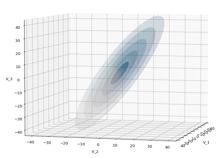
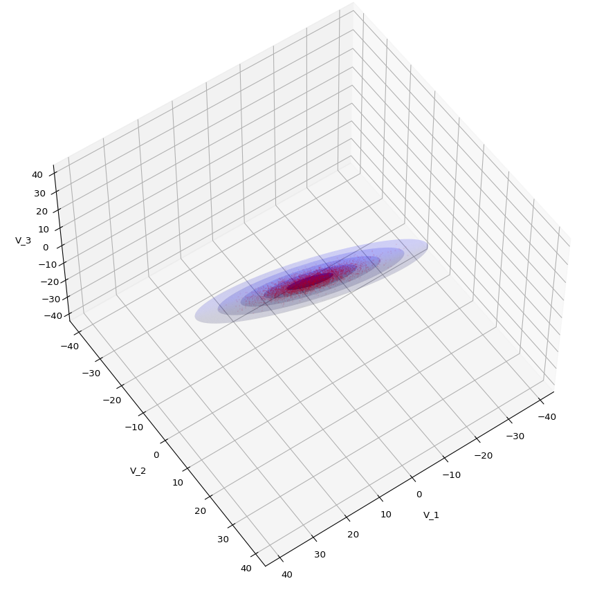
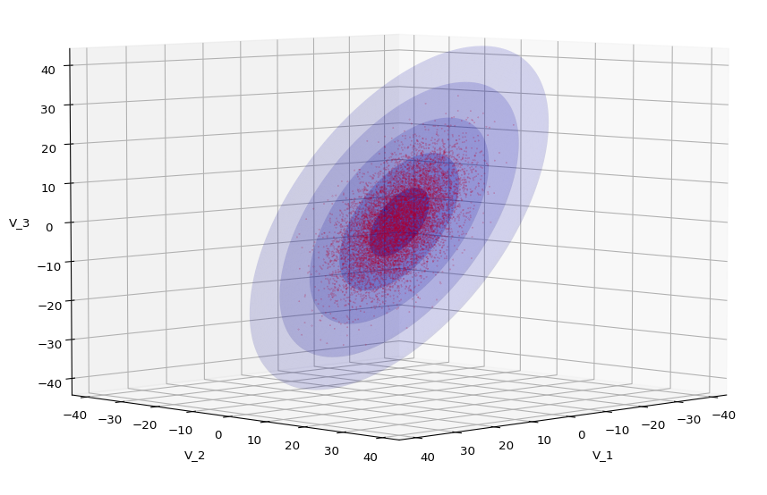
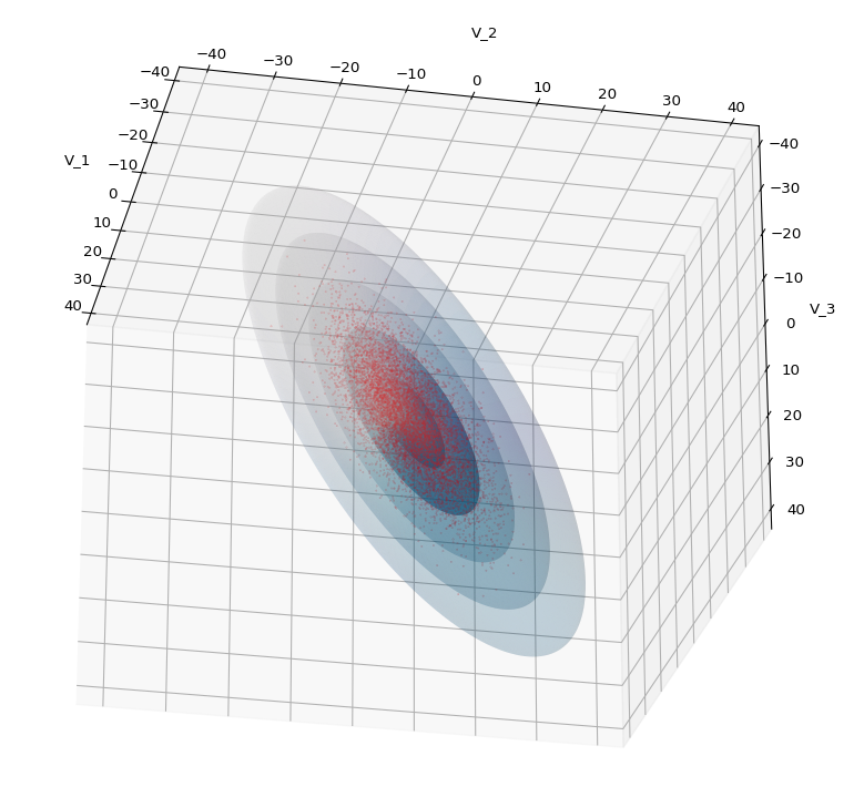
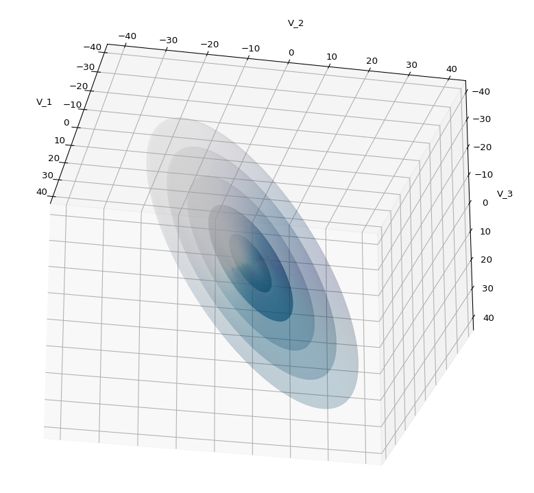
The result will be plots like the following:
The first plot combines a scatter plot of a TND with ellipsoidal contours. The 2nd plot only shows contours for confidence levels 1 ≤ σ ≤ 5 of our ideal TND. And I did a bit of shading.
How did I get there?
The covariance matrix determines everything
The mathematical object which characterizes the properties of a MND is its covariance matrix (Σ). Note that we can determine a (n x n)-covariance matrix for any X in n dimensions. Numpy provides a function cov() that helps you with this task. The relevant elements of the full covariance matrix for orthogonal projections into a 3-dim sub-space can be extracted (or better: cut out) by applying a suitable projection operator. This is trivial: Just select the elements with the (i, i)- and (i, j)-indices corresponding to the selected axes of the sub-space. The extracted 9 elements will then form the covariance matrix of the projected tri-variate distribution.
In case 2 we just define a (3 x 3)-Σ as the starting point of our work.
Let us assume that we got the essential Σ-matrix from an analysis of our distribution data or that we, in case 2, have created it. How does a (3 x 3)-Σ relate to ellipsoidal surfaces that show the same deformation and relations of the axes’ lengths as a corresponding tri-variate normal distribution?
Creation of a MND from a standardized normal distribution
In general any n-dim MND can be constructed from a standardized multivariate distribution of independent (and consequently uncorrelated) normal distributions along each axis. I.e. from n univariate marginal distributions. Let us call the standardized multivariate distribution SMND and its random vector Z. We use the coordinate system [CS] where the coordinate axes are aligned with the main axes of the SMND as the CS in which we later also will describe our given distribution X. Furthermore the origin of the CS shall be located such that the SMND is centered. I.e. the mean vector μ of the distribution shall coincide with the CS’s origin:
\[ \pmb{\mu} \: = \: \pmb{0}
\]
In this particular CS the (probability) density function f of Z is just a product of Gaussians gj(zj) in all dimensions with a mean at the origin and standard deviations σj = 1, for all j.
With z = (z1, z2, …, zn) being a position vector of a data point in the distribution, we have:
The construction recipe for the creation of a general MND XN from Z is just the application of a (non-singular) linear transformation. I.e. we apply a (n x n)-matrix onto the position vectors of the data points in the ℝn. Let us call this matrix A. I.e. we transform the random vector Z to a new random vector XN by
Σ determines the shape of the resulting probability distribution completely. We can reconstruct an A’ which produces the same distribution by an eigendecomposition of the matrix ΣX. A’ afterward appears as a combination of a rotation and a scaling. An eigendecomposition leads in general to
D contains the eigenvalues of Σ, whereas the columns of V are the components of the eigenvectors of Σ (in the present coordinate system). V represents a rotation and D a scaling.
The required transformation matrix T, which leads from the unrotated and unscaled SMND Z to the MND XN, can be rewritten as
The 1/2 abbreviates the square root of the matrix values (i.e. of the eigenvalues). A relevant condition is that ΣX is a symmetric and positive-definite matrix. Meaning: The original A itself must not be singular!
This works in n dimensions as well as in only 3.
Creation of a trivariate normal distribution
The creation of a centered tri-variate normal distribution is easy with Python and Numpy: We just can use
np.random.multivariate_normal( mean, Σ, m )
to create m statistical data points of the distribution. Σ must of course be delivered as a (3 x 3)-matrix – and it has to be positive definite. In the following example I have used
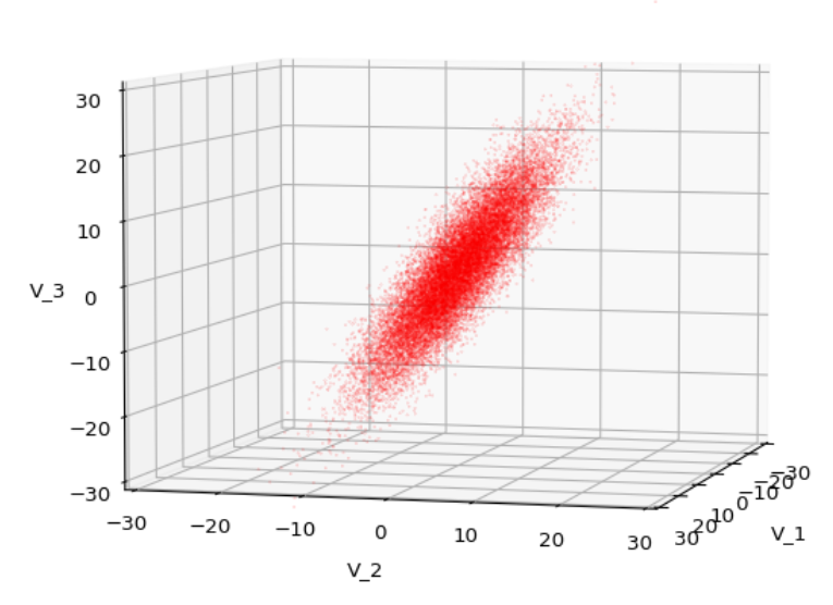
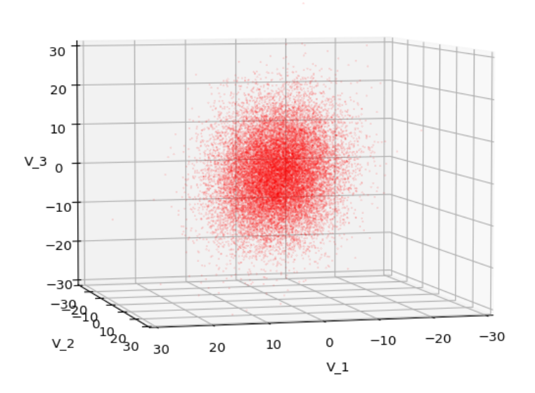
We have to feed this Σ-matrix directly into np.random.multivariate_normal(). The result with 20,000 data points looks like:
We see a dense inner core, clearly having an ellipsoidal shape. While the first image seems to indicate an overall slim ellipsoid, the second image reveals that our TND actually looks more like an extended lens with a diagonal orientation in the CS. =>
Note: When making such §D-plots we have to be careful not to make premature conclusions about the overall shape of the distribution! Projection effects may give us a wrong impression when looking from just one particular position and viewing angle onto the 3-dimensional distribution.
Create some nested transparent ellipsoidal surfaces
Especially in the outer regions the distribution looks a bit fluffy and not well defined. The reason is the density of points drops rapidly beyond a 3-σ-level. One gets the idea that a sequence of nested contour surfaces may be helpful to get a clearer image of the spatial distribution. We know already that contour surfaces of a MND are the surfaces of ellipsoids. How to get these surfaces?
The answer is rather simple: We just have to apply the mathematical recipe from above to specific data points. These data points must be located on the surface of a unit sphere (of the Z-distribution). Let us call an array with three rows for x-, y-, z-values and m columns for the amount of data points on the 3-dimensional unit sphere US. Then we need to perform the following transformation operation:
to get a valid distribution SX of points on the surface of an ellipsoid with the right orientation and relation of the main axes lengths. The surface of such an ellipsoid defines a contour surface of a TND with the covariance matrix Σ.
After the application of T to these special points we can use matplotlib’s
ax.plot_surface(x, y, z, …)
to get a continuous surface image.
To get multiple nested surfaces with growing diameters of the related ellipsoids we just have to scale (with growing and common integer factors applied to the σj-eigen-values).
Note that we must create all the surfaces transparent – otherwise we would not get a view to inner regions and other nested surfaces. See the code snippets below for more details.
SVD decomposition
We also have to get serious about numerically calculating T. I.e., we need a way to perform the “eigendecomposition”. Technically, we can use the so called “Singular Value Decomposition” [SVD] from Numpy’s linalg-module, which for symmetric matrices just becomes the eigendecomposition.
Code snippets
We can now write down some Jupyter cells with Python code to realize our SVD decomposition. I omit any functionality to project your real data into a 3-dim sub-space and to derive the covariance matrix. These are standard procedures in ML or statistics. But the following code snippets will show which libraries you need and the basic steps to create your plots. Instead of a general MND, I will create a TND for scatter plot points:
Code cell 1 – Imports
import numpy as np
import matplotlib as mpl
from matplotlib import pyplot as plt
from matplotlib.colors import ListedColormap
import matplotlib.patches as mpat
from matplotlib.patches import Ellipse
from matplotlib.colors import LightSource
Code cell 2 – Function to create points on a unit sphere
# Function to create points on unit sphere
def pts_on_unit_sphere(num=200, b_print=True):

    # Create pts on unit sphere
    u = np.linspace(0, 2 * np.pi, num)
    v = np.linspace(0, np.pi, num)

    x = np.outer(np.cos(u), np.sin(v))
    y = np.outer(np.sin(u), np.sin(v))
    z = np.outer(np.ones_like(u), np.cos(v))

    # Make array
    unit_sphere = np.stack((x, y, z), 0).reshape(3, -1)

    if b_print:
        print()
        print("Shapes of coordinate arrays : ", x.shape, y.shape, z.shape)
        print("Shape of unit sphere array : ",  unit_sphere.shape)
        print()

    return unit_sphere, x
Code cell 3 – Function to plot TND with ellipsoidal surfaces
# Function to plot a TND with supplied allipsoids based on the sam Sigma-matrix
def plot_TND_with_ellipsoids(elevation=5, azimuth=5,
                             size=12, dpi=96,
                             lim=30, dist=11,
                             X_pts_data=[],
                             li_ellipsoids=[],
                             li_alpha_ell=[],
                             b_scatter=False, b_surface=True,
                             b_shaded=False, b_common_rgb=True,
                             b_antialias=True,
                             pts_size=0.02, pts_alpha=0.8,
                             uniform_color='b', strid=1,
                             light_azim=65, light_alt=45
                            ):

    # Prepare figure
    plt.rcParams['figure.dpi'] = dpi
    fig = plt.figure(figsize=(size,size))  # Square figure
    ax = fig.add_subplot(111, projection='3d')

    # Check data
    if b_scatter:
        if len(X_pts_data) == 0:
            print("Error: No scatter points available")
            return

    if b_surface:
        if len(li_ellipsoids) == 0:
             print("Error: No ellipsoid points available")
             return
        if len(li_alpha_ell) < len(li_ellipsoids):
             print("Error: Not enough alpha values for ellipsoida")
             return
        num_ell = len(li_ellipsoids)

    # set limits on axes
    if b_surface:
        lim = lim * 1.7
    else:
        lim = lim

    # axes and labels
    ax.set_xlim(-lim, lim)
    ax.set_ylim(-lim, lim)
    ax.set_zlim(-lim, lim)
    ax.set_xlabel('V_1', labelpad=12.0)
    ax.set_ylabel('V_2', labelpad=12.0)
    ax.set_zlabel('V_3', labelpad=6.0)

    # scatter points of the MND
    if b_scatter:
        x = X_pts_data[:, 0]
        y = X_pts_data[:, 1]
        z = X_pts_data[:, 2]
        ax.scatter(x, y, z, c='r', marker='o', s=pts_size, alpha=pts_alpha)

    # ellipsoidal surfaces
    if b_surface:
        # Shaded
        if b_shaded:
            # Light source
            ls = LightSource(azdeg=light_azim, altdeg=light_alt)
            cm = plt.cm.PuBu
            li_rgb = []
            for i in range(0, num_ell):
                zz = li_ellipsoids[i][2,:]
                li_rgb.append(ls.shade(zz, cm))

            if b_common_rgb:
                for i in range(0, num_ell-1):
                    li_rgb[i] = li_rgb[num_ell-1]

            # plot the ellipsoidal surfaces
            for i in range(0, num_ell):
                ax.plot_surface(*li_ellipsoids[i],
                                rstride=strid, cstride=strid,
                                linewidth=0, antialiased=b_antialias,
                                facecolors=li_rgb[i],
                                alpha=li_alpha_ell[i]
                               )
        # just uniform color
        else:
            print("here")
            #ax.plot_surface(*ellipsoid, rstride=2, cstride=2, color='b', alpha=0.2)
            for i in range(0, num_ell):
                ax.plot_surface(*li_ellipsoids[i],
                                rstride=strid, cstride=strid,
                                color=uniform_color, alpha=li_alpha_ell[i])

    ax.view_init(elev=elevation, azim=azimuth)
    ax.dist = dist
    return
Some hints: The scatter data from the distribution X (or XN) must be provided as a Numpy array. The TND-ellipsoids and the respective alpha values must be provided as Python lists. Also the size and the alpha-values for the scatter points can be controlled. Reducing both can be helpful to get a glimpse also on ellipsoids within the relative dense core of the TND.
Some parameters as “elevation”, “azimuth”, “dist” help to control the viewing perspective. You can switch showing of the scatter data as well as ellipsoidal surfaces and their shading on and off by the Boolean parameters.
There are a lot of parameters to control a primitive kind of shading. You find the relevant information in the online documentation of matplotlib. The “strid” (stride) parameter should be set to 1 or 2. For slower CPUs one can also take higher values. One has to define a light-source and a rgb-value range for the z-values. You are free to use a different color-map instead of PuBu and make that a parameter, too.
Code cell 4 – Covariance matrix, SVD decomposition and derivation of the T-matrix
b_print = True

# Covariance matrix
cov1 = [[31.0, -4, 5], [-4, 26, 44], [5, 44, 85]]
cov = np.array(cov1)

# SVD Decomposition
U, S, Vt = np.linalg.svd(cov, full_matrices=True)
S_sqrt = np.sqrt(S)

# get the trafo matrix T = U*SQRT(S)
T = U * S_sqrt

# Print some info
if b_print:
    print("Shape U: ", U.shape, " :: Shape S: ", S.shape)
    print(" S      : ", S)
    print(" S_sqrt : ", S_sqrt)
    print()
    print(" U :\n", U)
    print(" T :\n", T)
Code cell 5 – Transformation of points on a unit sphere
# Transform pts from unit sphere onto surface of ellipsoids
# ~~~~~~~~~~~~~~~~~~~~~~~~~~~~~~~
b_print = True
num = 200
unit_sphere, xs = pts_on_unit_sphere(num=num)

# Apply transformation on data of unit sphere
ell_transf = T @ unit_sphere
# li_fact = [2.5, 3.5, 4.5, 5.5, 6.5]
li_fact = [1.0, 2.0, 3.0, 4.0, 5.0]
num_ell = len(li_fact)
li_ellipsoids = []
for i in range(0, num_ell):
    li_ellipsoids.append(li_fact[i] * ell_transf.reshape(3, *xs.shape))

if b_print:
    print("Shape ell_transf  : ", ell_transf.shape)
    print("Shape ell_transf0 : ", li_ellipsoids[0].shape)
Code cell 6 – TND data point creation and plotting
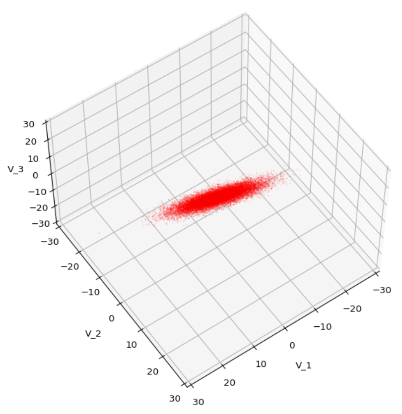
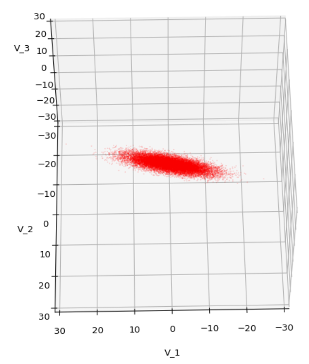
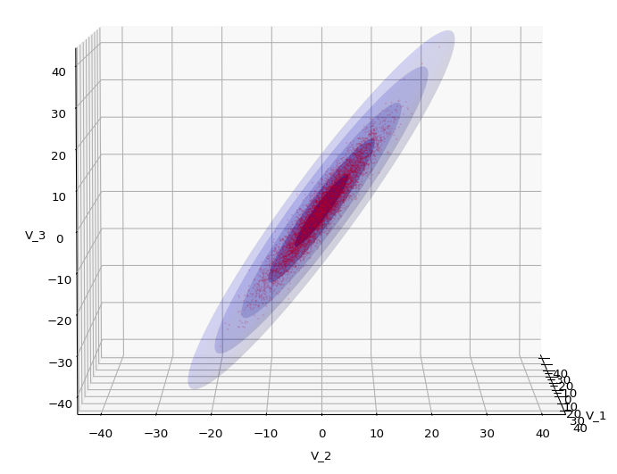
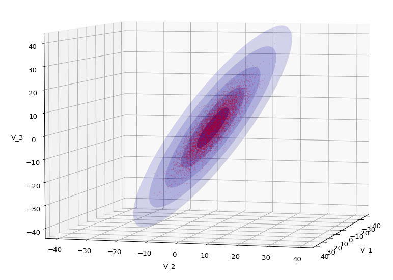
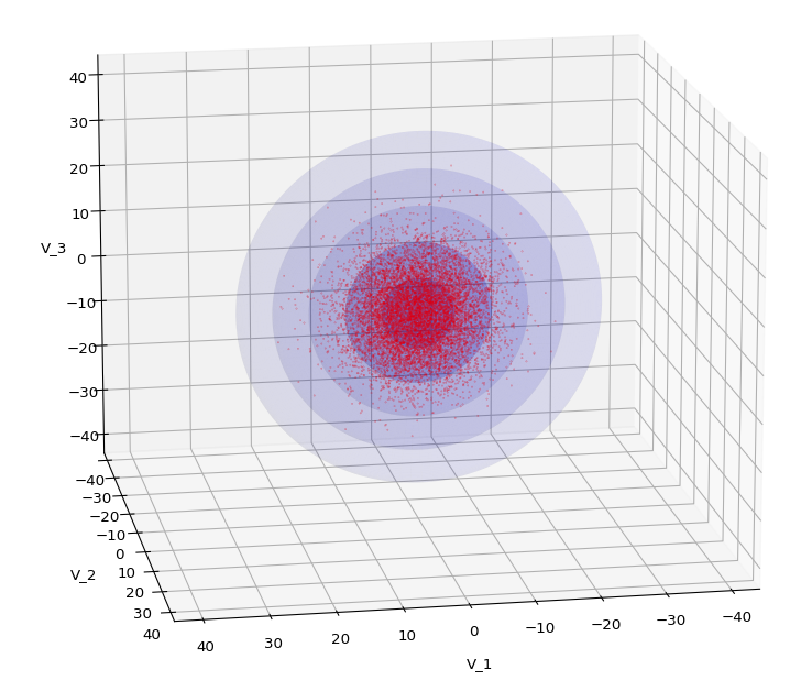
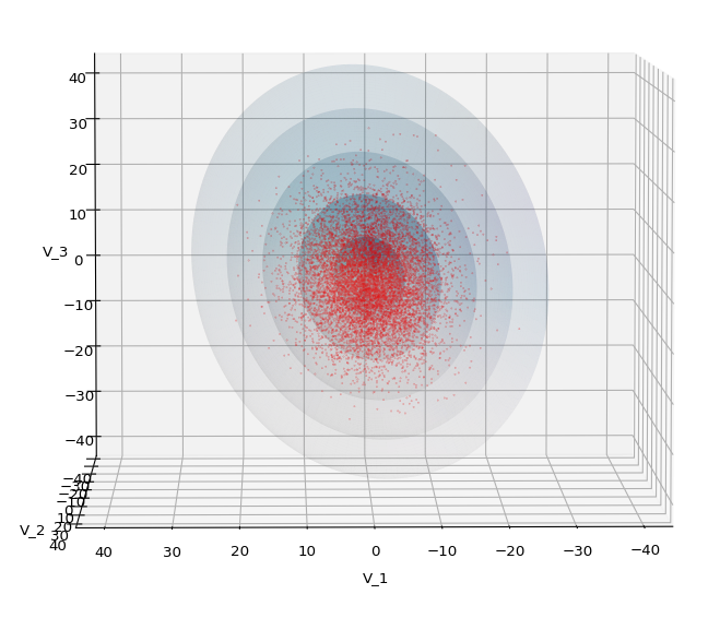
Let us play a bit around. The ellipsoidal contours are for σ = 1, 2, 3 ,4, 5. First we look at the data distribution from above. The ellipsoidal contours are for σ = 1, 2, 3 ,4, 5. We must reduce the size and alpha of the scatter points to 0.01 and 0.45, respectively, to still get an indication of the innermost ellipsoid of σ = 1. I used 8000 scatter points. The following plots show the same from different side perspectives – with and without shading and adapted alpha-values and number values for the scatter points
.
Yoo see: How a TND appears depends strongly on the viewing position. From some positions the distribution’s projection of the viewer’s background plane may even appear spherical. But on the other side it is remarkable how well the projection onto a background plane keeps up the ellipses of the projected outermost borders of the contour surfaces (of the ellipsoids for confidence levels). This is a dominant feature of MNDs in general.
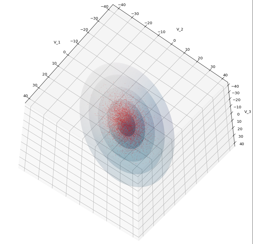
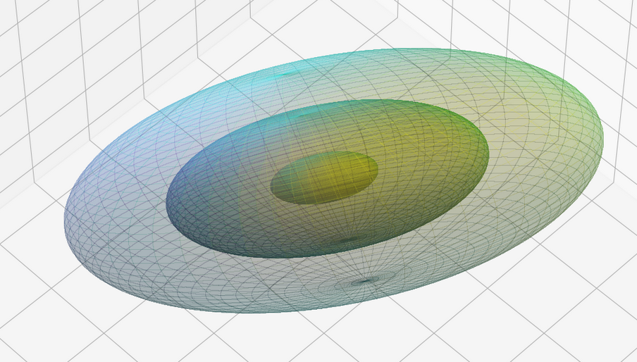
A last hint: To get a more volumetric impression it is required to both work with the position of the lightsource, the alpha-values and the colormap. In addition turning off ant-aliasing and setting the stride to something like 5 may be very helpful, too. The next image was done for an ellipsoid with slightly different extensions, only 3 ellipsoids and stride=5:
Conclusion
In this blog I have shown that we can display a tri-variate (normal) distribution, stemming from a construction of a standardized normal distribution or from a projection of some real data distribution, in 3D with the help of Numpy and matplotlib. As soon as we know the covariance matrix of our distribution we can add transparent surfaces of ellipsoids to our plots. These are constructed via a linear transformation of points on a unit sphere. The transformation matrix can be derived from an eigendecomposition of the covariance matrix.
The added ellipsoids help to better understand the shape and orientation of the tri-variate distribution. But plots from different viewing angles are required.
This post requires Javascript to display formulas!
Machine Learning [ML] algorithms are applied to multivariate data: Each individual object of interest (e.g. an image) is characterized by a set of n distinct and quantifiable variables. The variable values may e.g. come from measurements.
A sample of such objects corresponds to a data distribution in a multidimensional space, most often the ℝn. We can visualize our objects as data points in an Euclidean coordinate system of the ℝn: Each axis represents the values a specific variable can take; the position of a data point is given by the variable values.
Equivalently, we can use (position-) vectors to these data points. Thus, when training ML algorithms we typically deal with vector distributions, which by their very nature are multivariate. But also the outputs of some types of neural networks like Autoencoders [AE] form multivariate distributions in the networks’ latent spaces. For today’s ML-scenarios the number of dimensions n can become very big – even if we compress information in latent spaces. For a variety of tasks in generative ML we may need to understand the nature and shape of such distributions.
An elementary kind of a continuous multivariate vector distribution, for which major properties can be derived analytically, is the so called Multivariate Normal Distribution[MND]. MNDs, their marginal and their conditional distributions are of major importance both in the fields of statistics, Big Data and Machine Learning. One reason for this is the “central limit theorem” of statistics (in its vector form).
Some conventional ML-algorithms are even based on the assumption that the population behind the concrete data samples can be approximated by a MND. Due to the central limit theorem we find that averages of big samples of multivariate training data for a population of specific types of observed objects tend to form a MND. But also data samples in latent spaces of neural networks may show a multivariate normal distribution – at least in parts.
For the concrete problem of human face generation via a trained convolutional Autoencoder [CAE] I have actually found that the data produced in the CAE’s latent space can very well be described by a MND. See the posts on Autoencoders in this blog. This alone is motivation enough to dive a bit deeper into the (beautiful) mathematical properties of MNDs.
Just to illustrate it: The following plots show projections of the approximate MND onto coordinate planes.
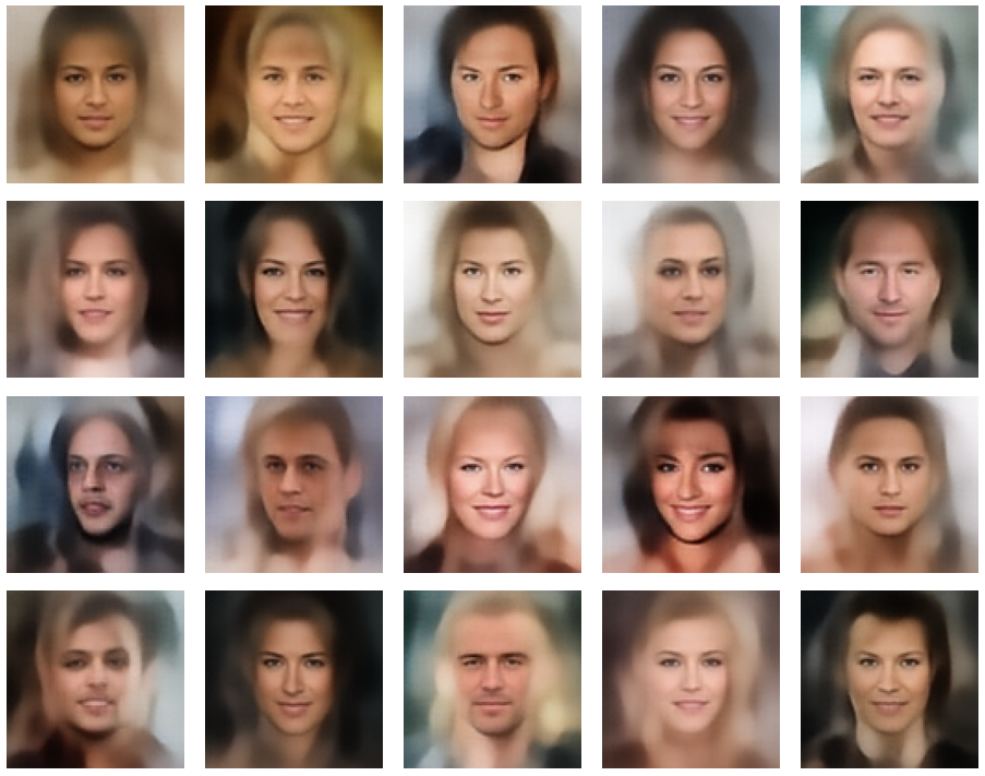
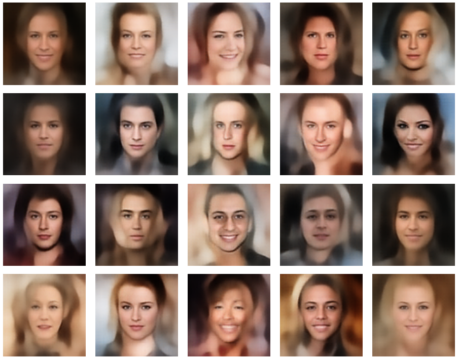
We find the typical elliptic contour lines which are to be expected for a MND. And here are some generated face images from statistical vectors which I derived from an analysis of the characteristic features of the 2-dim projections of the latent MND which my CAE had produced:
ML is math in the end – and MNDs are no exception
Some of my readers may have noticed that I wanted to start a series on the topic of creating random vectors for a given MND-like vector distribution. The characteristic parameters for the n-dimensional MND can either stem from an analysis of experimental ML data or come from theoretical sources. This was in April. But, I have been silent on this topic for a while.
The reason was that I got caught up in the study of the math of MNDs, of their properties, their marginal distributions and of quadratic forms in multiple dimensions (ellipsoids and ellipses). I had to re-collect a lot of mathematical information which I once (45 years ago) had learned at university. Unfortunately, multivariate analysis (i.e. data analysis in multidimensional spaces) requires some (undergraduate) university math. Regarding MNDs, knowledge both in linear algebra, statistics and vector analysis is required. In particular matrices, their decomposition and their geometrical interpretation play a major role. And when you try to understand a particular problem which obviously is characterized by an overlap of multiple mathematical disciplines the amount of information can quickly grow – without the connections and consistency becoming clear at first sight.
This is in part due to the different fields the authors of papers on MNDs work in and the different focuses they have on properties of MNDs. Although many introductory information about MNDs is available on the Internet, I have so far missed a coherent and comprehensive presentation which illustrates the theoretical insights by both ideal and real world examples. Too often the texts are restricted to pure formal derivations. And none of the texts discussed the problem of vector generation within the limits of MND confidence levels. But this task can become important in generative ML: At high confidence levels outliers become a strong weight – and deviations from an ideal MND may cause disturbances.
One problem with appropriate vector generation for creative ML purposes is that ML experiments deliver (latent) data which are difficult to analyze as they reside in high-dimensional spaces. Even if we already knew that they form a MND in some parts of a latent space we would have to perform a drill down to analytic formulas which describe limiting conditions for the components of the statistical vectors we want to create.
The other problem is that we need a solid understanding of confidence levels for a multidimensional distribution of data points, which we approximate by a MND. And on one’s way to understanding related properties of MNDs you pass a lot of interesting side aspects – e.g. degenerate distributions, matrix decompositions, affine transformations and projections of multidimensional hypersurfaces onto coordinate planes. Far too interesting to refrain from not writing something about it …
After having read many publicly available articles on MNDs and related math I had collected a bunch of notes, formulas and numerical experiments. The idea of a general post series on MNDs grew in parallel. From my own experiences I thought that ML people who are confronted with latent representations of data and find indications of a MND would like to have an introduction which covers the most relevant aspects of MNDs. On a certain mathematical level, and supported by illustrations from a concrete example.
But I will not forget about my original objective, namely the generation of random vectors within confidence levels. In the end we will find two possible approaches: One is based on a particular linear transformation, whose mathematical form is determined by a covariance analysis of our data distribution, and random number generators for multiple Gaussian distributions. The other solution is based on a derivation of precise conditions on random vector components from ellipses which are produced by projections of our real experimental data distribution onto coordinate planes. Such limiting conditions can be given in form of analytic expressions.
The second approach can also be understood as a reconstruction of a multivariate distribution from low-dimensional projection data:
We create vectors of a concrete MND-like vector distribution in n dimensions by only referring to characteristic data of its two-dimensional projections onto coordinate planes.
This is an interesting objective in itself as the access to and the analysis of 2-dimensional (correlated) data may be a much easier endeavour than analyzing the full distribution. But such an approach has to be supported by mathematical arguments.
Objectives of this post series
Objectives of this post series are:
We want to find out what a MND is in mathematical and statistical terms and how it can be based on a simpler vector distributions within the ℝn.
We want to study the basic role of a standardized multivariate normal distribution in the game and the impact of linear affine transformations on such a distribution – in terms of linear algebra and from a geometrical point of view.
We also want to describe and interpret the difference between normal MNDs and so called degenerate MNDs.
We want to understand the most important mathematical properties of MNDs. In particular we want to better grasp the mathematical meaning of correlations between the vector components and their impact on the probability density function. Furthermore the relation of a MND to its marginal distributions in sub-spaces of lower dimensions is of major interest.
We want to formally create a MND-approximation to a real multivariate data distribution by an analysis of real distribution’s properties and in particular from parameters describing the correlations between the vector components. Of particular interest are the covariance matrix and the precision or correlation matrix.
We want to study the role of projections when turning from a MND to its marginal distributions and the impact of such projections on the matrices qualifying the original and its marginal distributions.
We want to understand the form of contour hyper-surfaces for constant probability density values of a MND. We also want to derive what the projections of these hyper-surfaces onto coordinate planes look like.
We want to show that both contour hyper-surfaces of the MND and of its projections in marginal distributions contain the same proportions of integrated data points and, equivalently, the same probability proportions resulting from an integration of the probability density from the distribution’s center up to the hyper-surfaces.
We want to illustrate basic MND-creation principles and the effects of linear affine transformations during the construction process by an ideal 3-dimensional MND example and by projections of a real vector distribution from an ML-experiment onto 2-dimensional and 3-dimensional sub-spaces. We also want to illustrate the relation between the MND and its marginal distributions by plotting concrete 3-dimensional examples and their projections onto coordinate planes.
We want to use the derived MND properties for the creation of statistical vectors v which fulfill the following conditions:
Each of the generated v is a member of a vector population, which has been derived from a ML experiment and which to a good approximation can be described by a MND (and its extracted basic parameters).
Each v has an endpoint within the multidimensional volume enclosed by a contour-hypersurface of the MND’s probability density function [p.d.f.],
The limiting hypersurface is defined by a chosen confidence level.
We want to create statistical vectors within the limit of contour hyper-surfaces by using elementary construction principles of a MND.
In a second approach we want to reduce vector creation to solving a sequence of 2-dimensional problems. I.e. we want to work with 2-dim marginal distributions in 2-dim sub-spaces of the ℝn. We hope that the probability density functions of the relevant distributions can be described analytically and provide computable limiting conditions on vector components. Note: The production of statistical vectors from data of projected low-dimensional marginal distributions corresponds to a reconstruction of the full MND from its projections.
During random vector creation we want to avoid PCA-transformations of the whole real data distribution or of projections of it.
Based on MND-parameters we want to find analytic expressions for the vector component limits whenever possible.
The attentive reader has noticed that the list above includes an assumption – namely that a multidimensional contour hypersurface of a MND can be associated with something like a confidence level. In addition we have to justify mathematically that the reduction to data of 2-dimensional projections of the full vector distribution is a real option for statistical vector creation.
The last three points are a bit tough: Even if we believe in math textbooks and get limiting hyper-curves of a quadratic form in our coordinate planes the main axes of the respective ellipses may show angles versus the coordinate axes (see the example images above). All this would have to be taken care of in a precise analytic form of the limits which we impose on the components of our aspired statistical vectors.
So, this series is, at least in parts, going to be a tough, but also very satisfactory journey. Eventually, after having clarified diverse properties of MNDs and their marginal distributions in lower dimensional spaces, we will end up with quadratic equations and some simple matrix operations.
Objectives of the next post
We must not forget that statistics plays a major role in our business. In ML we deal with finite collections (samples) of individual object data which are statistically picked from a greater population (with assumed statistical properties). An example is a concrete collection of images of human faces and/or their latent vectors. The data can be organized in form of a two-dimensional data matrix: Its rows may indicate individual objects and its columns properties of these objects (or vice versa). In either direction we have vectors which focus on a particular aspect of the data: Individual objects or the statistics of a specific object property.
While we are used to univariate “random variables” we have to turn to so called “random vectors” to describe multidimensional statistical distributions and respective samples picked from an underlying population. A proper vector notation will give us the advantage of writing down linear transformations of a whole multidimensional vector distribution in a short and concise form.
Besides introducing random vectors and their components the next post
will also discuss related probability densities, expectation values and the definition of a covariance matrix for a random vector. Some simple properties of the covariance matrix will help us in further posts.
This post requires Javascript to display formulas!
Convolutional Autoencoders and multivariate normal distributions
Experiments as with my own on convolutional Autoencoders [CAE] show: A CAE maps a training set of human face images (e.g. CelebA) onto an approximate multivariate vector distribution in the CAE’s latent space Z. Each image corresponds to a point (z-point) and a corresponding vector (z-vector) in the CAE’s multidimensional latent space. More precisely the results of numerical experiments showed:
The multidimensional density function which describes the inner dense core of the z-point distribution (containing more than 80% of all points) was (aside of normalization factors) equivalent to the density function of a multivariate normal distribution[MND] for the respective z-vectors in an Euclidean coordinate system.
After a normalization with an appropriate factor the continuous density functions controlling the multivariate vector distribution can be interpreted as a probability density function [p.d.f.]. The components vj (j=1, 2,…, n) of the vectors to the z-points are regarded as logically separate, but not uncorrelated variables. For each of these variables a component specific value distribution Vj is given. All these marginal distributions contribute to a random vector distribution V, in our case with the properties of a MND:
μ is a vector with all mean values μj of the Vj component distributions as its components. Σ abbreviates the covariance matrix relating the distributions Vj with one another.
The point distribution of a CAE’s MND forms a complex rotated multidimensional ellipsoid with its center somewhere off the origin in the latent space. The latent space itself typically has many dimensions. In the case of my numerical experiments the number of dimension was n ≥ 256. The number of sample vectors used were between 80,000 and 200,000 – enough data to approximate the vector distribution by a continuous density function. The densities for the Vj-distributions formed a smooth Gaussian function (for a reasonable sampling interval). But note: One has to be careful: The fact that the Vj have a Gaussian form is not a sufficient condition for a MND. (See the next post.) But if a MND is given all Vj have a Gaussian form.
Generative use of MNDs in multidimensional latent spaces of high dimensionality
When we want to use a CAE as a generative tool we need to solve a problem: We must create statistical vectors which point into the (multidimensional) volume of our point distribution in the latent space of the encoding algorithm. Only such vectors provide useful information to the Decoder of the CAE. A full multivariate normal distribution and hyperplanes of its multidimensional density function are difficult to analyze and to control when developing a proper numerical algorithm. Therefore I want to reduce the problem of vector generation to a sequence of viewable and controllable 2-dimensional problems. How can this be achieved?
A central property of a multivariate normal distribution helps: Any sub-selection of m vector-component distributions forms a multivariate normal distribution, too (see below). For m=2 and for vector components indexed by (j,k) with respective distributions Vj, Vk we get a so called “bivariate normal distribution” [BND]:
for vector component values vj, vk defines a point density of the sample data in the (j,k)-coordinate plane of the Euclidean coordinate system in which the MND is described. The density function of the marginal distributions Vj showed the typical Gaussian forms of a univariate normal distribution.
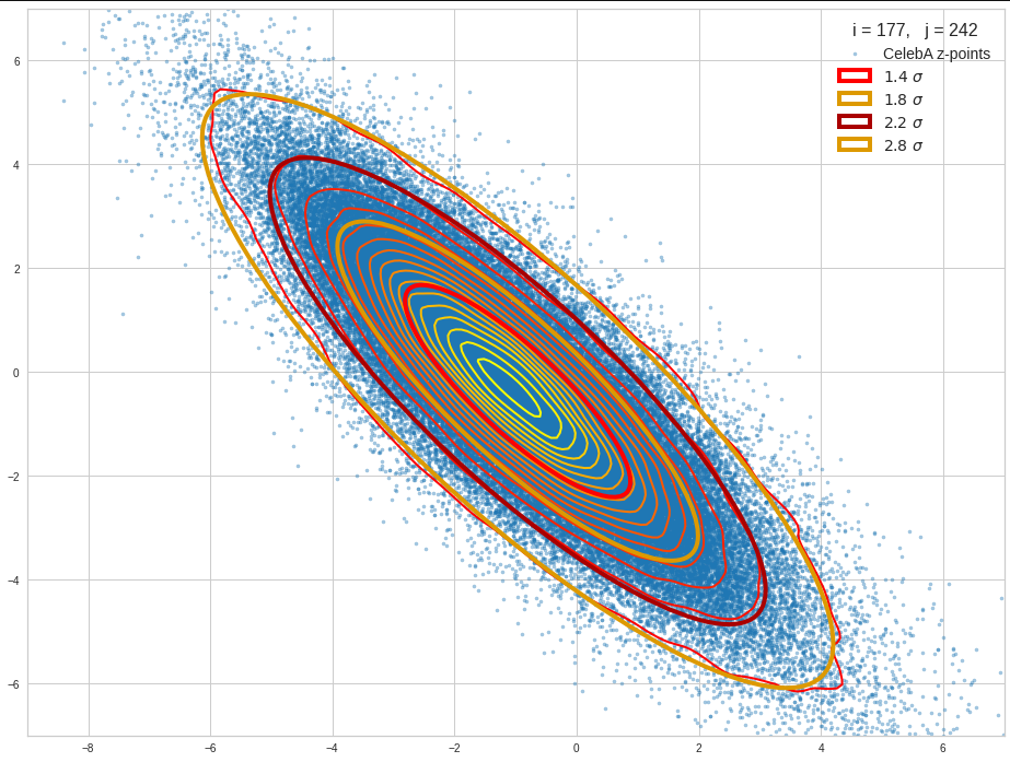
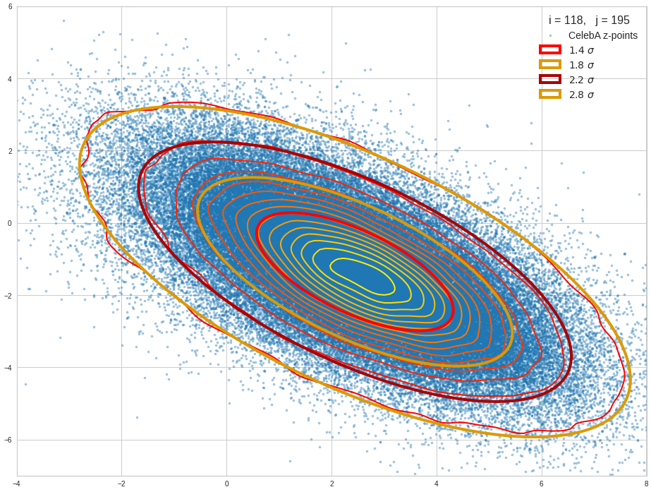
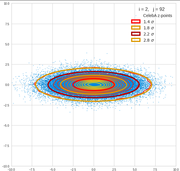
The density function of a BND has some interesting mathematical properties. Among other things: The hyperplanes of constant density of a BND’s density function form ellipses. This is illustrated by the following plots showing such contour lines for selected pairs (Vj, Vk) of a real point-distribution in a 256-dimensional latent space. The point distribution was created by a CAE in its latent space for the CelebA dataset.
Contour lines for selected (j,k)-pairs. The thick lines stem from theory and calculated correlation coefficients of the univariate distributions.
The next plot shows the contours of selected vector-component pairs after a PCA-transformation of the full MND. (Main ellipse axes are now aligned with the axes of the PCA-coordinate system):
These ellipses with axes along the coordinate axes are relatively easy to handle. They can be used for vector creation. But they require a full PCA transformation of the MND-distribution, a PCA-analysis for complexity reduction and an application of the inverse PCA-transformation. The plot below shows the point-density compared to a 2.2-σ-confidence ellipses. The orange points are the results of a proper statistical numerical vector generation algorithm based on a PCA-transformation of the MND.
See my post quoted above for the application of a PCA-transformation of the multidimensional MND for vector creation.
However, we get the impression that we could also use these rotated ellipses in projections of the MND onto coordinate planes of the original latent space system directly to impose limiting conditions on the component values of statistical vectors pointing to an inner regions of the MND. Of course, a generated statistical vector must then comply with the conditions of all such ellipses. This requires an analysis and combined use of the ellipses of all of the subordinate BNDs of a the original MND during an iterative or successive definition of the values for the vector components.
Objective of this post series
In my last post about CAEs (see the link given above) I have explicitly asked the question whether one can avoid performing a full PCA-transformation of the MND when creating statistical vectors pointing to a defined inner region of a MND.
The objective of this post series is to prove the answer: Yes, we can. And we will use the BNDs resulting from projections of the original MND onto coordinate planes. We will in particular explore the n*(n-1)/2 the properties of the BNDs’ confidence ellipses. As said: These ellipses are rotated against the coordinate system’s axes. We will have to deal with this in detail. We will also use properties of their 1-dimensional marginal distributions (projections onto the coordinate axes, i.e. the Vj.)
In addition we need to prepare a variety of formulas before we are able to define numerical procedure for the vector generation without a full PCA-transformation of the MND with around 100,000 vectors. Some of the derived formulas will also allow for a deeper insight into how the multiple BNDs of a MND are related between each other and with confidence hypersurfaces of the MND.
Ellipses in general lead to equations governed by quadratic or fourth power polynomials. We will in addition use some elementary correlation formula from statistics and for some exercises a simple optimization via derivatives. The series can be regarded as an excursion into some of the math which governs bivariate distributions resulting from a MND.
As MNDs may also be the result of other generative Machine Learning algorithms in respective latent spaces, the whole approach to statistical vector generation for such cases should be of general interest. Note also that the so called “central limit theorem” almost guarantees the appearance of MNDs in many multivariate datasets with sufficiently large samples and value dependencies on many singular observations.
Distributions of a variety of variables may result in a MND if the variables themselves depend on many individual observables with limited covariance values of their distributions. In particular pairwise linearly correlated Gaussian density distributions individual variables (seen as vector components) may constitute a MND if the conditional probabilities fulfill some rules. We will see a glimpse of this in 2 dimensions when we analyze integrals over Gaussians in the bivariate normal case.
Other approaches to statistical vector generation?
Well, we could try to reconstruct the multidimensional density function of the MND. This is a challenge which appears in some problems of pure statistics, but also in experimental physics. See e.g. a paper of Rafey Anwar, Madeline Hamilton, Pavel M. Nadolsky (2019, Department of Physics, Southern Methodist University, Dallas; https://arxiv.org/pdf/1901.05511.pdf). Then we would have to find the elements of the (inverse) covariance matrix or – equivalently – the elements of a multidimensional rotation matrix. But the most efficient algorithms to get the matrix coefficients again work with projections onto coordinate planes. I prefer to use properties of the ellipses of the bivariate distributions directly.
Note that using the multidimensional density function of the MND directly is not of much help if we want to keep the vectors’ end points within a defined multidimensional inner region of the distribution. E.g.: You want to limit the vectors to some confidence region of the MND, i.e. to keep them inside a certain multidimensional ellipsoidal contour hyper-surface. The BND-ellipses in the coordinate planes reflect the multidimensional ellipsoidally shaped contour hyperplanes of the full distribution. Actually, when we vertically project a multidimensional hyperplane onto a coordinate plane then the outer 2-dim border line coincides with a contour ellipse of the respective BND. (This is due to properties of a MND. We will come back to this in a future post.) The problem of proper limiting individual vector component values thus again is best solved by analyzing properties of the BNDs.
Steps, methods, mathematical level
As a first step I will, for the sake of completeness, write down the formula for a multivariate normal distribution, discuss a bit its mathematical construction from uncorrelated univariate normal distribution. I will also list up some basic properties of a MND (without proof!). These properties will justify our approach to create statistical vectors pointing into a defined inner region of the MND by investigating projected contour ellipses of all subordinate BNDs. As a special aspect I want to make it at least plausible, why the projected contour ellipses define infinitesimal regions of the same relative probability level as their multidimensional counterparts – namely the multidimensional ellipsoidal hypersurfaces which were projected onto coordinate planes.
Then as a first productive step I want to motivate the specific mathematical form of the probability density function [p.d.f] of a bivariate normal distribution. In contrast to many of the math papers I have read on the topic I want to use a symmetry argument to derive the basic form of the p.d.f. I will point out an important, but plausible assumption about conditional distributions. An analogous assumption on the multidimensional level is central for the properties of a MND.
As the distributions Vj and Vk can be correlated we then want to understand the impact of the correlation coefficients on the parameters of the 2-dimensional density function. To achieve this I will again derive the density function by using our previous central assumption and some simple relations between the expectation values of the constituting two univariate distributions in the linear correlation regime. This concludes the part of the series where we get familiar with BNDs.
Furthermore we are interested in features and consequences of the 2-dimensional density functions. The contour lines of the 2-dim density function are ellipses – rotated by some specific angle. I will look at a formal mathematical process to construct such ellipses – in particular confidence ellipses. I will refer to the results Carsten Schelp has provided in an Internet article on this topic.
His construction process starts with a basic ellipse, which I will call base correlation ellipse[BCE]. The length of the axes of this ellipse are eigenvalues of the covariance matrix of the standardized marginal distributions constituting the BND. The main axes of this elementary ellipse are in addition aligned with the two selected axes of a basic Euclidean coordinate system in which the bivariate distribution is defined. The length of the BCE’s main axes can be shown to depend on the correlation coefficient for the two vector component distributions Vj and Vk. This coefficient also appears in the precision matrix of the BND. Points on the base correlation ellipse can be mapped with two steps of an affine transformation onto points on the real contour ellipses, in particular to points of the confidence ellipses.
The whole construction process is not only of immense help when designing visualization programs for the contour ellipses of our distribution with many (around 100,000) individual vectors. The process itself gives us some direct geometrical insights. It also helps to avoid finding a numerical solution of the usual eigenvector-problems when answering some specific questions about the rotated contour ellipses. Normally we solve an eigenvalue-problem for the covariance matrix of the multi- or the many subordinate bi-variate distributions to get precise information about contour ellipses. This corresponds to a transformation of the distributions to a new coordinate system whose axes are aligned to the main axes of the ellipses. Numerically this transformation is directly related to a PCA transformation of the vector distributions. However, such a PCA-transformation can be costly in terms of CPU time.
Instead, we only need a numerical determination of all the mutual the correlation coefficients of the univariate marginal distributions of the MND. Then the eigenvalue problem on the BND-level is already analytically solved. We therefore neither perform a full numerical PCA analysis of the MND and multidimensional rotation of the vectors of around 100,000 samples. Nor do we analyze explained variance ratios to determine the most important PCA components for dimensionality reduction. We neither need to perform a numerical PCA analysis of the BNDs.
Most important: Our problem of vector generation is formulated in the original latent space coordinate system and it gets a direct solution there. The nice thing is that Schelp’s construction mechanism reduces the math to the solution of quadratic polynomial equations for the BNDs. The solutions of those equations, which are required for our ultimate purpose of vector generation, can be stated in an explicit form.
Therefore, the math in this series will mostly remain on high school level (at least at a level given when I was young). Actually, it was fun to dive back into exercises reminding me of school 50 years ago. I hope the interested reader has some fun, too.
Solutions to some particular problems with respect to the confidence ellipses of the MND’s BNDs
In particular we will solve the following problems:
Problem 1: The two points on the BCE-ellipse with the same vj-value are not mapped onto points with the same vj-value on the confidence ellipse. We therefore derive the coordinates of points on the BCE-ellipse that give us one and the same vj-value on the real confidence ellipse.
Problem 2: Plots for a real MND vector distribution indicate that all (n-1) confidence ellipses of distribution pairs of a common Vj with other marginal distributions Vk (for the same confidence level and with k ≠ j) have a common tangent parallel to one coordinate axis. We will derive the value of a maximum v_j-value for all ellipses of (j,k)-pairs of vector component distributions. We will prove that it is identical for all k. This will define the common interval of allowed vj-component-values for a bunch of confidence ellipses for all (Vj, Vk)-pairs with a common Vj.
Problem 3: The BCE-ellipses for a common j-, but different k-values depend on different values for the correlation coefficients ρj,k of Vj with its various Vk counterparts. Therefore we need a formula that relates a point on the BCE-ellipse leading to a concrete v_j-value of the mapped point on the confidence ellipse of a particular (Vj, Vk)-pair to respective points on other BCE-ellipses of different (Vj, Vm)-pair with the same resulting v_j-value on their confidence ellipses. I will derive such a formula. It will help us to apply multiple conditions onto the vector component values.
Problem 4: As a supplemental exercise we will derive a mathematical expression for the size of the main axes and the rotation angle of the ellipses. We should, of course, get values that are identical to results of the eigenwert-problem for the correlation matrix (describing a PCA coordinate transformation). This gives us additional confidence in Schelps’ approach.
In the end we can use our results to define a numerical algorithm for the direct creation of vectors pointing to a defined inner region of the multivariate normal distribution. As said, this algorithms does not require a costly PCA transformations of the full MND or many, namely n*(n-1)/2 such PCA-transformations of its BNDs.
I intend to visualize all results with the help of a concrete example of a multivariate example distribution created by a CAE for the CelebA dataset. The plots will use Schelp’s construction algorithm for the confidence ellipses extensively.
Conclusion and outlook
Convolutional Autoencoders create approximate multivariate normal distributions [MND] for certain input data (with Gaussian pattern properties) in their latent space. MNDs appear in other contexts of machine learning and statistics, too. For evaluation and generative purposes one may need statistical vectors with end points inside a defined multidimensional hypersurface corresponding to a certain confidence level and a certain constant density value of the MND’s density function. These hypersurfaces are multidimensional ellipsoids.
We have the hope that we can use mathematical properties of the MND’s subordinate bivariate normal distributions [BNDs] to create statistical vectors with end points inside the multidimensional confidence ellipsoids of a MND. Typically such an ellipsoid resides off the origin of the latent space’s coordinate system and the ellipsoid’s main axes are rotated against the axes of the coordinate system. We intend to base the confining conditions on the components of the aspired statistical vectors on correlation coefficients of the marginal vector component distributions. Our numerical algorithm should avoid a full PCA-transformation of the multidimensional vector distribution.
In the next post of this series I give a formula for the density function of a multivariate normal distribution. In addition I will list up some basic properties which justify the vector generation approach via bivariate normal distributions.