This post requires Javascript to display formulas!
In the two previous posts of this series
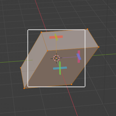
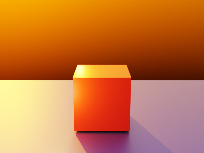
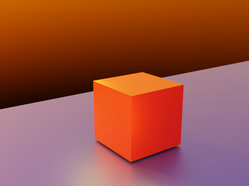
Fun with shear operations and SVD – I – shear matrices and examples created with Blender
Fun with shear operations and SVD – II – Shearing of rectangles and cubes with Python and Matplotlib
we have clarified some basic properties of shear transformations [SHT]. We got interested in this topic, because Autoencoders can produce latent multivariate normal vector distributions, which in turn result from linear transformations of multivariate standard normal distributions. When we want to analyze such latent vector distributions we should be aware transformations of quadratic forms. An important linear transformation is a shear operation. It combines aspects of scaling with rotations.
The objects we applied SHTs to were so far only squares and cubes. Both (discrete) rotational and plane symmetries of the squares and cubes were broken by SHTs. We also saw that this symmetry breaking could not be explained by a pure scaling operation in another rotated Euclidean Coordinate System [ECS]. But cubes do not have a continuous rotational symmetry. The distances of surface points of a cube to its symmetry center show no isotropy.
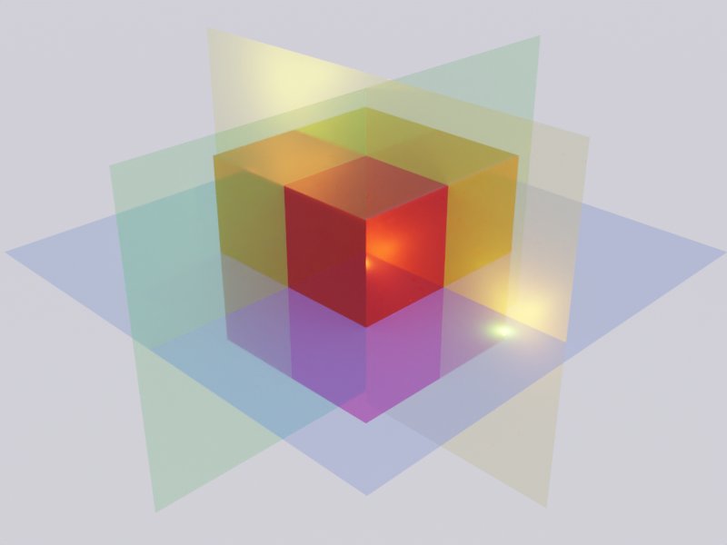
However, already in the first post when we superficially worked with Blender we got the impression that the shearing of a sphere seemed to produce a figure with both plane and discrete rotational symmetries – namely ellipsoids, wich appeared to be rotated. We still have to prove this, mathematically. With this post we move a first step in this direction: We will apply a shear operation to a 2D-body with perfect continuous rotational symmetry in all directions, namely a circle. A circle is a special example of a quadratic form (with respect to the vector component values). We center our Euclidean Coordinate System [ECS] at the center of the circle. We know already that this point remains a fix-point of our transformations. As in the previous post I use Python and Matplotlib to produce visual results. But we support our impression also by some simple math.
We first check via plotting that the shear operations move an extremal point of the circle (with respect to the y-coordinate) along a line ymax = const. (Points of other layers for other values yl = const also move along their level-lines.) We then have to find out whether the produced figure really is an ellipse. We do so by mathematically deriving its quadratic form with respect to the coordinates of the transformed points. Afterward, we derive the coordinate values of points with extremal y-values after the shear transformation.
In addition we calculate the position of the points with maximum and minimum distance from the center. I.e., we derive the coordinates of end-points of the main axes of the ellipse. This will enable us to calculate the angle, by which the ellipse is rotated against the x-axis.
The astonishing thing is that our ellipse actually can be created by a pure scaling operation in a rotated ECS. This seems to be in contrast to our insight in previous posts that a shear matrix cannot be diagonalized. But it isn’t … It is just the rotational symmetry of the circle that saves us.
Shearing a circle
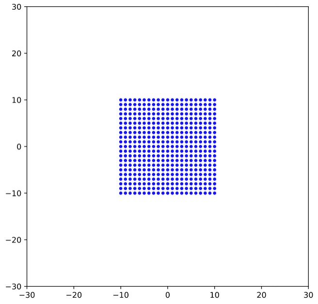
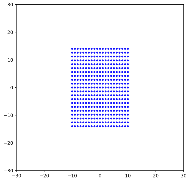
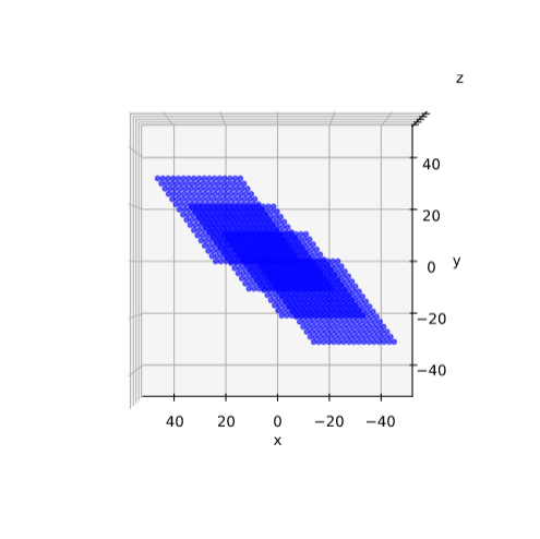
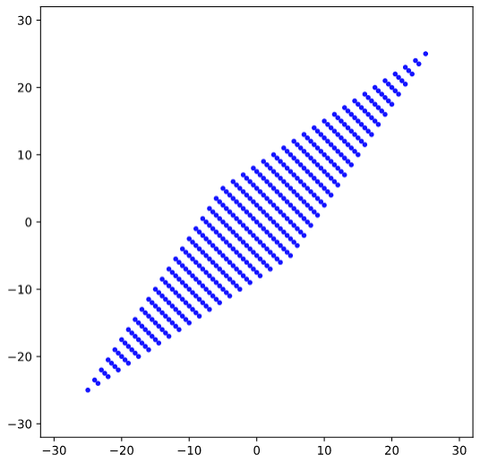
We define a circle with radius r = a = 2.
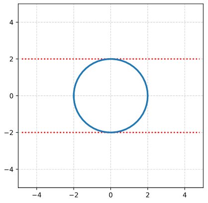
I have indicated the limiting line at the extremal y-values. From the analysis in the last post we expect that a shear operation moves the extremal points along this line.
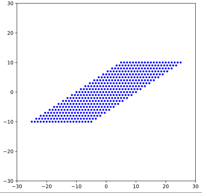
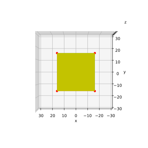
We now apply a shearing matrix with a x/y-shearing parameter λ = 2.0
\]
The result is:
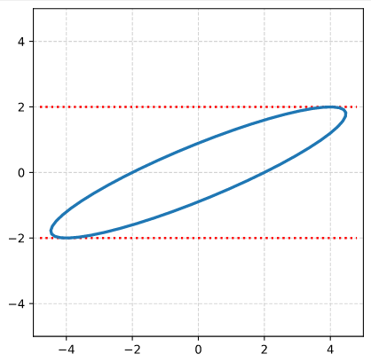
As expected! This really looks like an ellipse. Can we proof it?
Transformation of the circle
We use the definition of a shear transformation in 2D (see the first post of this series):
x_s \: &= \: x \, + \, \lambda * y \\
y_s \: &= \: y
\end{align}
\]
and the definition of the original circle with radius a:
{x^2 \over \, a^2} \, + \, {y^2 \over \, a^2} \:&=\: 1 \\
\Rightarrow \: {x_s^2 \,-\, λ y_s \over \, a^2} \, + \, {y_s^2 \over \, a^2} \:&=\: 1 \phantom{\Huge{(}}
\end{align}
\]
This actually gives us a quadratic expression in the new coordinate values:
x_s^2 \, + \, \left(\,1\,+\,\lambda^2\, \right)*y_s^2 \:-\: {2 \lambda \over 1\,+\,\lambda^2}*x_s*y_s \:=\: a^2
\]
Thus, we have indeed produced a rotated ellipse! We see this from the fact that the term mixing the xs and the yl coordinates does not vanish.
Position of maximum absolute y-values
We know already that the y-coordinates of the extremal points (in y-direction) are preserved. And we know that these points were located at x = 0, y = a. So, we can calculate the coordinates of the shifted point very easily:
\]
In our case this gives us a position at (4, 2). But for getting some experience with the quadratic form let us determine it differently, namely by rewriting the above quadratic equation and by a subsequent differentiation. Quadratic supplementation gives us:
\left[\, y_s \,- \, {\lambda \over 1\,+\, \lambda^2} \, x_s^2 \, \right]^2 \:=\:
{ 1 \over \left( 1\,+\, \lambda^2 \right)^2} \left[\, a^2\left(\, 1\,+\,\lambda^2 \,\right) \, – \, x_s^2 \,\right],
\]
y_s \:=\: {1 \over 1\,+\, \lambda^2}\, \left( \, \lambda x_s \, \pm \, \left[\, a^2\left(\, 1\,+\,\lambda^2 \,\right) \, – \, x_s^2 \,\right]^{1/2}\, \right)
\]
and
{\partial y_s \over \partial x_s } \:=\: {1 \over 1\,+\, \lambda^2 }\, \left( \, \lambda \, \pm \, {(-x_s) \over \left[\, a^2\left(\, 1\,+\,\lambda^2 \,\right) \, – \, x_s^2 \,\right]^{1/2} } \, \right)
\]
We demand that the derivative becomes zero:
{\partial y_s \over \partial x_s } \:=\: 0 \: \Rightarrow \: x_s^2 \, = \, \lambda^2 \, \left[\, a^2\left(\, 1\,+\,\lambda^2 \,\right) \, – \, x_s^2 \,\right]
\]
Thus – as expected :
x_s^2 \, = \, \lambda^2 \, a^2
\]
Points with maximum radial distance
Let us also find the position of the end-points of the main axes of the ellipse. One method would be to express the ellipse in terms of the coordinates (xs, ys), calculate the squared radial distance rs of a point from the center and set the derivative with respect to xs to zero.
r_s^2 \, = \, x_s^2 \, +\, \left(y_s(x_s)\right)^2, \quad {\partial r_s \over \partial x_s} \,= \, 0 \,.
\]
The “problem” with this approach is that we have to work with a lot of terms with square roots. Sometimes it is easier to just work in the original coordinates and express everything in terms of (x, y):
r_s^2(x) \, = \, \left(x_s(x)\right)^2 \, +\, \left(y_s(x)\right)^2, \quad {\partial r_s(x) \over \partial x} \,= \, 0 \,.
\]
With the basic circle equation and the transformation rules this gives us:
{\partial \over \partial x} \left[x^2 \,+\, 2 \lambda x y \,+\, \lambda^2 y^2 \,+\, y^2 \right] \,= \, 0
\]
\quad {\partial \over \partial x} \left[a^2(1 \,+\ \lambda^2) \,-\, \lambda^2 x^2 + 2 \lambda x \left(a^2\,-\, x^2\right)^{1/2} \right] \,= \, 0
\]
We do not get rid of the square roots. But it is easy to handle. Sorting of terms and getting rid of the denominator leads us to
\left( a^2\,-\ x^2 \right) \, =\, x^2 \,+\, \lambda x \left( a^2 \,-\, x^2 \right)^{1/2}
\]
Adding a quadratic supplementation term gives:
\left( a^2\,-\ x^2 \right) \,+\, {\lambda^2 \over 4} \left( a^2\,-\ x^2 \right) \, =\, \left[ \, x \,+\, {\lambda \over 2 } \left( a^2 \,-\, x^2 \right)^{1/2} \, \right]^2
\]
Taking the square root and reordering results in:
x \,=\, \left( a^2 \,-\, x^2 \right)^{1/2} \, \left[\,\pm\, \left( 1\,+\, {\lambda^2 \over 4} \right) ^{1/2} -\, {\lambda \over 2} \,\right]
\]
Squaring leads to:
x^2 \,&=\, \left( a^2 \,-\, x^2 \right) \, \left[\,1 \,+\, {1 \over 2} \lambda^2 \,\pm\, {\lambda \over 2} \left(4\,+\, \lambda^2\right)^{1/2} \,\right] \\
&:=\ \xi * \left( a^2 \,-\, x^2 \right)
\end{align}
\]
So, in the end, we get a very simple expression for the x-coordinate of the axes’ end-points:
x \,=\, \pm\, a\, \sqrt{\eta \phantom{\large{(}} }, \quad \mbox{with} \quad \eta \,=\, {\xi \over 1\, +\, \xi }
\]
This gives us all in all 4 solutions as ξ got two values:
\xi_1 \,&=\, \left[\,1 \,+\, {1 \over 2} \lambda^2 \,-\, {\lambda \over 2} \left(4\,+\, \lambda^2\right)^{1/2} \,\right], \quad \eta_1 \, = \, {\xi_1 \over 1\, +\, \xi_1} \\
\xi_2 \,&=\, \left[\,1 \,+\, {1 \over 2} \lambda^2 \,+\, {\lambda \over 2} \left(4\,+\, \lambda^2\right)^{1/2} \,\right], \quad \eta_2 \, = \, {\xi_2 \over 1 \,+\, \xi_2}
\end{align}
\]
This was to be expected as there are 4 end-points of 2 main axes of an ellipse.
Of course, we need the transformed coordinates. A small calculation shows:
End points of 1st main axis
x_{s1} \,&=\,\, \: a\, \sqrt{\eta_1 \phantom{\large{(}} } \,+\, \lambda a \, \sqrt{1 \,-\,\eta_1 \phantom{\large{(}} }, \quad
y_{s1} \,=\, \: a\, \sqrt{1 \,-\,\eta_1 \phantom{\large{(}} } \\
x_{s2} \,&=\, – a \, \sqrt{\eta_1 \phantom{\large{(}} } \,-\, \lambda a \, \sqrt{1 \,-\,\eta_1 \phantom{\large{(}} }, \quad
y_{s2} \,=\, – a \, \sqrt{1 \,-\,\eta_1 \phantom{\large{(}} }
\end{align}
\]
End points of 2nd main axis
x_{s3} \,&=\,\,\: a \, \sqrt{\eta_2 \phantom{\large{(}} } \,-\, \lambda a \, \sqrt{1 \,-\,\eta_2 \phantom{\large{(}} }, \quad
y_{s3} \,=\, – \, a \, \sqrt{1 \,-\,\eta_2 \phantom{\large{(}} } \\
x_{s4} \,&=\, – a \, \sqrt{\eta_2 \phantom{\large{(}} } \,+\, \lambda a \, \sqrt{1 \,-\,\eta_2 \phantom{\large{(}} }, \quad
y_{s4} \,=\,\, \: a \, \sqrt{1 \,-\,\eta_2 \phantom{\large{(}} } \\
\end{align}
\]
These formulas enable us also to calculate the length-values of our ellipse’s main axes (half-diameters!), as and bs :
a_s \,&=\,\,\: \sqrt{\,x_{s1}^2 \, + \, y_{s1}^2 \phantom{\large{(}} }, \quad \left(\,\approx 4.83 \,\right) \\
b_s \,&=\,\,\: \sqrt{\,x_{s3}^2 \, + \, y_{s3}^2 \phantom{\large{(}} }, \quad \left(\,\approx 0.83\, \right)
\end{align}
\]
For our shearing in x-direction as gives us the longer axis. The rotational angle α between the longer main axis and the x-axis can be calculated via:
\alpha \,=\, \arctan \left( { y_{s1} \over x_{s1} } \right) , \quad \left( \,\approx 22.5 \deg \right)
\]
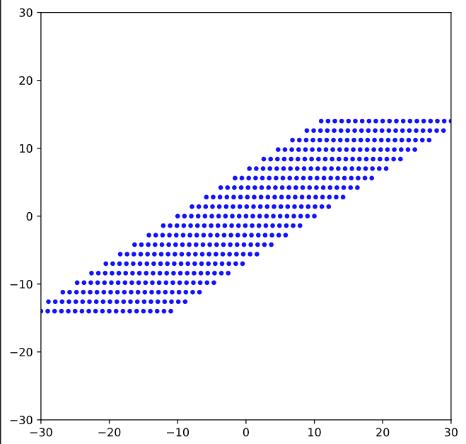
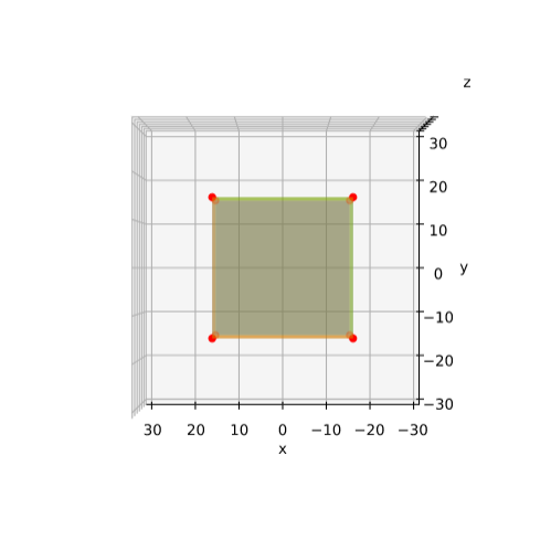
Plot of main axes, their end-points and of the points with maximum y-value
The coordinate data found above help us to plot the respective points and the axes of the produced ellipse. The diameters’ end-points are plotted in red, the points with extremal y-value in green:
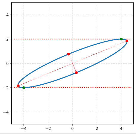
It becomes very clear that the points with maximum y-values are not identical with the end-points of the ellipse’s main symmetry axes. We have to keep this in mind for a discussion of higher dimensional figures and vector distributions as multidimensional spheres, ellipsoids and multivariate normal distributions in later posts.
Rotated ECS to produce the ellipse?
The plot above makes it clear that we could have created the ellipse also by switching to an ECS rotated by the angle α. Followed by a simple scaling in x- and y-direction by the factors as and bs in the rotated ECS. This seems to be a contradiction to a previous statement in this post series, which said that a shear matrix cannot be diagonalized. We saw that in general we cannot find a rotated ECS, in which the shear transformation reduces to pure scaling along the coordinate axes. We assumed from linear algebra that we in general need a first rotation plus a scaling and afterward a second different rotation.
But the reader has already guessed it: For a fully rotation-symmetric, i.e. isotropic body any first rotation does not change the figure’s symmetry with respect to the new coordinate axes. In contrast e.g. to squares or rectangles any rotated coordinate system is as good as any other with respect to the effect of scaling. So, it is just scaling and rotating or vice versa. No second rotation required. We shall in a later post see that this holds in general for isotropically shaped bodies.
Conclusion
Enough for today. We have shown that a shear transformation applied to a circle always produces an ellipse. We were able to derive the vectors to the points with maximum y-values from the parameters of the original circle and of the shear matrix. We saw that due to the circle’s isotropy we could reduce the effect of shearing to a scaling plus one rotation or vice versa. In contrast to what we saw for a cube in the previous post.
In the next post
Fun with shear operations and SVD – IV – Shearing of ellipses
we will apply a shearing transformation to an ellipse.